O
pen
A
rchive
T
OULOUSE
A
rchive
O
uverte (
OATAO
)
OATAO is an open access repository that collects the work of Toulouse researchers and
makes it freely available over the web where possible.
This is an author-deposited version published in :
http://oatao.univ-toulouse.fr/
Eprints ID : 12348
To link to this article : DOI :10.1016/j.envsoft.2012.11.003
URL :
http://dx.doi.org/10.1016/j.envsoft.2012.11.003
To cite this version : Caillault, Sébastien and Miahle, François and
Vannier, Clémence and Delmotte, Sylvestre and Kedowide, Conchita
and Amblard, Fredéric and Etienne, Michel and Becu, Nicolas and
Gautreau, Pierre and Houet, Thomas
Influence of incentive networks on
landscape changes: A simple agent-based simulation approach. (2013)
Environmental Modelling and Software, vol. 45. pp. 64-73. ISSN
1364-8152
Any correspondance concerning this service should be sent to the repository
administrator:
[email protected]
Influence of incentive networks on landscape changes: A simple
agent-based simulation approach
q
S. Caillault
a
, F. Mialhe
b
, C. Vannier
c
, S. Delmotte
d
, C. Kêdowidé
e
, F. Amblard
f
,
M. Etienne
g
, N. Bécu
h
, P. Gautreau
b
, T. Houet
i
,*
aGEOPHEN UMR 6554 LETG, Université de Caen Basse-Normandie, BP8156, 14032 Caen Cedex, France
bPRODIG UMR 8586 CNRS, Université Panthéon-Sorbonne/Denis Diderot, 5 rue Thomas Mann, 75013 Paris, France cCOSTEL UMR 6554 LETG CNRS, Université de Rennes, Pl. Du recteur Henri Le Moal, 35043 Rennes, France dINRA UMR Innovation, 2 Place Pierre Viala, 34070 Montpellier Cedex, France
eENeC UMR 8185 CNRS, Universités Paris 8, 2 rue de la Liberté, 93526 Saint-Denis, France fIRIT-UT1, Université de Toulouse 1, 2 rue doyen Gabriel Marty, 31042 Toulouse Cedex 9, France gINRA Avignon, Unité Ecodéveloppement, Site Agroparc, 84914 Avignon Cedex 9, France hPRODIG UMR 8586 CNRS, Université Panthéon-Sorbonne, 2 rue Valette, 75005 Paris, France
iGEODE UMR 5602 CNRS, Université de Toulouse, 5 allée Antonio Machado, 31058 Toulouse Cedex, France
a b s t r a c t
The aim of this paper is to implement a simple model for exploring the influence of different multi-scale incentive networks affecting farmer decision on landscape changes. Three scales of networks are considered: a global ‘policy’ network promoting specific land uses, an intermediate ‘social’ network where land use practices are shared and promoted collectively and a local ‘neighborhood’ network where land use practices are influenced by those of their neighbors. We assess the respective and combined influence of these networks on landscape pattern (fragmentation and heterogeneity) and dynamics, taking into account agronomic constraints (assimilated to crop successions). Simulations show that combination of incentive networks does not have linear and/or cumulative influence on landscape changes. Comparison of simulated scenarios highlights that a combination of two networks tends to improve landscape heterogeneity and fragmentation; scenarios combining all networks could lead to two opposite landscape configuration illustrating emergence of landscape dynamics. Finally, this study emphasizes that landscape complexity has also to be understood through the multiplicity of pathways of landscape changes rather than the assessment of the resulting landscape patterns.
1. Introduction
Land use/cover change (LUCC) is the result of the interaction
between humans and their environment. The impact of agriculture
is unparalleled to other LUCC in its combination of spatial extent
and intensity of influence (
Lambin et al., 2001
). Agricultural
development has induced dramatic consequences on habitats,
water quality, and biodiversity (
Butler et al., 2007
;
Gordon et al.,
2008
) by modifying landscape patterns (i.e. composition and
structure) and hydro-chemical processes (nutrient cycles, etc.).
LUCC comes from the actions and interactions of different
stake-holders operating at different levels who are continuously
influ-encing the structure and composition of the landscape (
Valbuena
et al., 2010
). Agricultural landscape patterns are driven by
multi-scale forces e from the global economy, international policies,
and soil properties at regional, farm and field scale, to local social
choices and individual practices (
Veldkamp et al., 2001
). An
increasing number of agricultural products are now embedded
in global commodity chains, i.e. “a network, or rather a set of
networks, and processes that result in an end-product or
commodity and linking labor, production, households, states, and
enterprises to one another within the global economy” (
Gereffi and
Korzeniewicz, 1994
). Such a global network provokes production
and practice changes in response to social, environmental and
economic demands from different stakeholders at different scales.
In contrast, local factors, such as the “neighborhood,” are still
influential and explain the diffusion by contagion of farming
innovations (
Daudé, 2004
). Intermediate scale factors e regional or
national e such as union membership, may also influence the
decisions of farmers concerning their land uses. Farming decisions
q Thematic Issue on Spatial Agent-Based Models for Socio-Ecological Systems. * Corresponding author. Tel.: þ33 (0)5 61 50 36 28; fax: þ33 (0)5 61 50 42 75.
result from the internal representations and beliefs of farmers that
may evolve with information given and diffused by other farmers,
institutions, associations and other networks (
Wauters et al., 2010
).
Thus, most LUCC in rural regions occurs at the farm scale where
these driving forces are integrated (
Kristensen et al., 2001
;
Baudry
and Thenail, 2004
).
Landscape change models are particularly appropriate for
testing and assessing the influence of social, economic and
ecological processes, their dynamics, and interactions that modify
landscape patterns (
Baker, 1989
;
Gaucherel and Houet, 2009
;
Zimmerman, 2008
). A common approach to simulating LUCC as
a consequence of collective or individual decisions and actions is
through the use of agent-based models (ABM) (
Matthews et al.,
2007
;
Parker et al., 2003, 2008
;
Robinson et al., 2007
;
Treuil
et al., 2008
). ABMs are particularly well suited to modeling
different types of networks that can lead to the emergence of new
spatial patterns (
Bretagnolle et al., 2000
;
Gimblett, 2001
;
Urbani,
2006
). ABMs help to assess the influence of land use policies, the
interactions between land uses (
Rouan et al., 2012
), on
socio-ecological systems based on different scenarios (
Le et al., 2010
;
Parry et al., 2012
;
Robinson et al., 2012
) but also to identify possible
land use strategies based on the companion modelling framework
(
Etienne, 2006
;
Simon and Etienne, 2010
). Because the driving
forces of LUCC in agricultural landscapes are numerous and act at
multiple scales (
Bürgi et al., 2004
), the assessment of their
respective and combined influence still remains a challenge.
Although landscapes exhibit a hierarchical structure (
Burel and
Baudry, 2003
), the modeling of involved multi-scale processes
has not always lead to the simulation of realistic landscapes. Thus,
land use systems are characterized by complex interactions
between human decision-making and their biophysical
environ-ment (
Smajgl et al., 2011
). LUCC ABMs are particularly well suited
for representing complex spatial interactions under heterogeneous
conditions and for modeling decentralized, autonomous
decision-making (
Parker et al., 2003
). Furthermore, the use of neutral
landscape models (
Gardner et al., 1987
;
O’Neill et al., 1992
), which
are simple models applied on theoretical landscapes, has been
recognized as a potential technique for better understanding of
landscape dynamics (
Gaucherel et al., 2006
). These models help to
include and study the interactions between multiple driving forces
and thus are able to tackle the complexity of the processes involved
(
McAllister et al., 2005
;
Houet et al., 2010b
), as the use of ABMs on
neutral landscapes shows promising results (
Brown et al., 2004
).
The aim of this paper is to implement a theoretical e neutral e
model for exploring the influence of different multi-scale incentive
networks, both individually and in various combinations, on
land-scape pattern and dynamics. An incentive network is defined as
a social network, composed by individuals and/or institutions
among which information is diffused to favor a certain action/
decision to promote a land use type. In our model, three scaled
networks influence farmers’ decisions: a global ‘policy’ network
promoting specific land uses through incentives to farmers, an
intermediate ‘social’ network where land use practices are shared
and promoted collectively, and a local ‘neighborhood’ network
where the land use practices are influenced by those of their
neighbors. This multi-layered network approach is quite original in
the field of LUCC/landscape modelling and shows some similarities
to studies modelling some social relations in the landscape (
Berger,
2001
;
IMAGES, 2004
).
2. Methodology: model description and experiments
The NetLogo platform (version 4.1 eWilensky, 1999) has been used to develop the IRIUS model (Impact des Réseaux d’Influence sur l’Utilisation du Sol i.e. Impact of incentive networks on land use). Its description follows the ODD protocol (Grimm et al., 2006, 2010).
2.1. Overview 2.1.1. Purpose
The purpose of this model is to explore and assess the impact of different and multi-scale incentive networks that operate at three scales (global, social and neighborhood) on farmers’ land use decision-making and consequently on land-scape pattern.
2.1.2. Entities
The model includes various entities:
- ‘farmers’ (agents/individuals). Agents have limited cognitive capacities. They have to respect agronomic constraints (crop succession). After receiving incentives of land use types from networks, they prioritize them according to the agronomic constraints related to crops succession and choose the highest recommended one. In case of contradictory incentives, they can choose a convenient land use type randomly.
- ‘farm’ (spatial units). Each farm belongs to a farmer. The overall landscape is composed of all spatial units. Each spatial unit has two state variables: land use type and age. The land use type is approached under a simplified represen-tation with a numerical code (1, 2 or 3) that is initially randomly assigned to each spatial entity. Land use types change over time according to farmer decisions and agronomic constraints. Such constraints define the maximum duration of each land use type (‘age’) accordingly toCastellazzi et al. (2008,
2010)and Houet et al. (2010a). When the maximum value of the age is
reached, the current land use type must change to one of the two other possible land use types.
- ‘global network’ (environment). This entity simulates a public policy encour-aging farmers to adopt specific land use practices according to a global land use assessment made at the landscape scale. The network is composed of all farmers, who all receive the same incentive from this global e public policy e entity. - ‘social network’ (collective). This entity simulates voluntary membership in
formal or informal associations (e.g. farmers’ unions, lobbies, etc.) that influ-ence farmers’ practices. All farmers belong to one of the five user-defined social groups, each encompassing equal proportions of farmers.
- ‘local network’ (collective). This entity intends to simulate the influence of neighbors’ land use practices. Indeed, some authors have shown that some local land use changes could occur for various e environmental or economic e reasons (Daudé, 2004). The diffusion of such land uses changes is theoretically explained by the imitation and adoption by one farmer of the most common practice that occurs in the neighboring farms (Gotts and Polhill, 2009;
Kaufmann et al., 2009), even if this effect is sometimes hard to detect in reality
(Schmit and Rounsevell, 2006). As such, each farmer tends to adopt the
dominant land use within his neighborhood, represented in the network by the eight adjacent farms (Moore neighborhood).
2.1.3. Spatial and temporal scales
The model is run for 250 time steps, where one time step corresponds to one cropping season (which could represent as much as one year or as few as several months). The landscape is composed of 25 " 25 spatial units, or 625 farms. To avoid border effects, the local network is defined by the Moore neighborhood of each cell within a torus space (Kimura, 2002).
2.1.4. Process overview and scheduling
At each time step, each farmer receives an incentive from each network that encourages him to produce or adopt a specific land use type. According to the age of the current land use, each farmer lists the possible land use types that he is able to implement. A set of decision rules is used to simulate the decision-making of farmers to choose a land use type for the next time step based on the received incentives. The landscape is updated with new land uses implemented within each cell. 2.2. Design concepts
2.2.1. Basic principles
The interest of this study lies in the simple model which allows for testing of all possible combinations of networks and assessing their influence on landscape pattern and dynamics.
2.2.2. Emergence
Emergence may occur by specific combinations of initial situations and network incentives. The local network tends to homogenize practices locally. The global network favors less frequent land use types by giving feedback on previous land uses. The social network influences the practices of groups of farmers. The generated landscape configuration is not predictable and strongly depends on the initial randomized distribution of social networks and on initial randomized landscape configuration. According to the initial conditions and the number and type of active networks during the simulation, landscape patterns could emerge from individual-based decisions.
2.2.3. Adaptation
Farmers do not have a wide range of possible decisions. They adopt the land use type suggested by the majority of the networks if it is consistent with the agronomic constraints. If not, the remaining recommended land use type is adopted. No indi-vidual initiative in the choice of land use type is simulated.
2.2.4. Objectives
Networks incite farmers to adopt the land use type that are recommended to them. ‘Local’ and ‘social’ networks encourage farmers to adopt the land use type used by the majority of their respective members (e.g. to maximize agricultural production). The ‘global’ network analysis in which the land use types are less represented at the landscape scale incites all farmers to adopt it (e.g. to improve landscape heterogeneity at an aggregated level to favor biodiversity preservation) (Poiani et al., 2000;Lindenmayer et al., 2006).
2.2.5. Learning
Neither farmers nor networks change their behavior according to their experience.
2.2.6. Prediction
No prediction activity is realized by any kind of agent or entity in the model. 2.2.7. Sensing
Farmers directly receive recommendations from ‘social’ and ‘global’ networks for a specific land use type. They themselves calculate the major land use type in their neighborhood, and use the result as a recommendation from the ‘local’ network to adopt this land use.
2.2.8. Interaction
Farmers react to incentives given by the ‘global’ and ‘social’ networks while they have direct (neighboring) interactions within their local network.
2.2.9. Stochasticity
We assume that landscape configuration at the initial step does not strongly affect landscape dynamics. As randomness occurs at the initialization, the modeler can only specify land use ratios. The land use attribute and age of each cell are randomly allocated. The farmers’ membership to a social group is also randomly chosen. Randomness also occurs while running the model: a ‘blank’ land use recommendation may be sent (e.g. no land use type is favored). In such case, farmers would randomly choose a land use type among the possible land use type list. This case occurs for example when the three networks send the same incentives, i.e. suggest the same land use type (e.g. 2e2e2) to a farm that has already reached its maximum land use age under that proposed configuration.
2.2.10. Observation
Assessing the influence of networks on landscape dynamics (Gustafson, 1998) is carried out using two quantitative indices: the Shannon Diversity Index (SDI) and the Patch Density Index (PDI). This is a standard way of analyzing landscape structure in landscape ecology (O’Neill et al., 1988;Burel and Baudry, 2003). The SDI is described byFormula (1)and gives a synthetic value of landscape heterogeneity. The PDI describing landscape fragmentation simply equals the number of landscape patches for each land use type. A landscape patch is composed by identical contiguous landscape units (i.e. land use type).
SDI ¼XS
i¼1ðpi$lnðpiÞÞ (1)
pie the number of spatial units (farms) of land-use type “i” over the total number of spatial units
S e total number of land-use types
Landscape pattern is considered here from the point of view of the combined evolution of landscape fragmentation and heterogeneity. A mean value of landscape heterogeneity and fragmentation is computed from the simulations made for each scenario. To assess and characterize the influence of each/combined network(s) on landscape pattern (heterogeneity and fragmentation), we used standard scores of these landscape indices. To exclude cases where class frequency is “0” (Ln 0 is impossible) we add 0.0001 for all classes in the formula, what explains why SDI is sometimes superior to 1. These values of landscape heterogeneity and fragmentation make all scenarios comparable.
2.3. Details 2.3.1. Initialization
All simulations were run with an equal ratio of land use types. The number of social groups is user-defined, but was fixed to five in this study. Farmers are randomly assigned to one of the social groups which finally show equal numbers of farmers (125 here). The maximum ‘age’ for each land use can be selected from two possible values (5 or 10). The age of each land use (between 1 and the selected
maximum age value) is randomly assigned for each cell. Finally, a user can activate (or not) the influence of one or several networks.
2.3.2. Input data
The model does not use external data sources. 2.3.3. Submodels
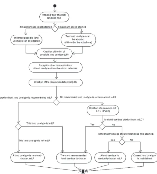
Creation, diffusion and processing (decision) of information are the main operators of the existing submodels. At every time step, farmers receive incentives from the networks in a single list, called a ‘recommendation list’. Then, a new list of information is created according to current land use age, called a ‘list of possibilities’.
Fig. 1summarizes submodels implementation.
- The global network favors the minor land use at the landscape scale to maxi-mize landscape diversity according toDeke (2008). Land use proportions are calculated for each time step. If two minor land uses are equal, the global network does not recommend any land use.
- The local network reproduces a common farmer behavior that consists of imitating the most frequent agricultural practices in his neighborhood (Deffuant et al., 2002;Kaufmann et al., 2009). For each farmer, land use ratios are computed for the eight adjacent farms and the most frequent land use is recommended. In the case that two land uses occur equally in the neighbor-hood, the local network does not recommend any land uses.
- The social network is promoting a common land use practice that is the most frequent within the social group each farm belongs to. It somehow replicates the impact of innovative land use practices diffusion (Saltiel et al., 1994). If two land use types are dominant, the social network does not recommend any land use type.
- The farmer’s decision rule performs as follows: if the “recommendation list” contains a dominant land use type, and if this type is in the “list of possibilities” the farmer chooses it. If the “recommendation list” does not provide any land use recommendation (all null), the farmer randomly chooses a land use type from the list of possibilities. If the “recommendation list” does not contain a dominant land use type, it is randomly chosen from land use types listed in the list of possibilities (Fig. 1).
3. Experiments
Three kinds of experiments can be distinguished. First, type
behaviors (in terms of landscape heterogeneity) are identified and
characterized from the simulations. Then, some runs were made to
assess model sensitivity to initial landscape configuration. Finally,
some others, called scenarios, for evaluating the respective and
combined influence of networks on landscape pattern and
dynamics.
In a first step the observed behaviors from the outputs of the
simulations were qualified. The term ‘behavior’ is used to
charac-terize an evolution of the SDI in term of magnitude, variability and
trend. Secondly, to assess model sensitivity to initial landscape
configuration we designed an experiment to estimate the influence
of initial land use and age patterns on results. The experiment
crossed two archetypal initial configurations of land use spatial
distribution (a scattered distribution versus a perfectly aggregated
one
1) and two configurations for the initial age distribution (a
random one versus age of all spatial units set to one). The influence
of the initial spatial distribution for the social groups is not assessed
as it does not evolve during the simulation and can thus be
considered as a static variable. We therefore use the same random
spatial distribution of the social groups for all the initial
configu-rations tested. Each initial configuration is simulated 100 times.
Thirdly, the respective and combined influence of networks on
landscape pattern is assessed through the simulation of eight
scenarios.
Table 1
presents all scenarios and illustrates all possible
combinations of networks. Each scenario is simulated 40 times, i.e.
with 40 different initial configurations, to assess landscape changes
variability. Scenarios are analyzed in the light of these behaviors to
1For the scattered distribution, the landscape is generated randomly, yet
respecting equal distribution of each use. For the aggregated one, the land-scape is split into three equal stripes, one for each land-use.
answer the following question: Does a scenario lead to a specific
landscape heterogeneity behavior? We therefore study the
influ-ence of networks on landscape pattern (i.e. from the point of
view of the combined evolution of landscape fragmentation and
heterogeneity).
As detailed in paragraphs 2.1.3, 2.3.1 and 2.3.3, all other
parameters are kept constant along the experimental design. The
environment is a regular torus of 25*25 (625 farms). The three land
use types are equally represented and randomly allocated at the
initialization. The number of social groups is kept constant to 5.
Initial landscape and social network configurations remain the
same for all scenarios.
4. Results
4.1. Behaviors of landscape heterogeneity from simulations
All simulations allow the identification of six main types of
‘behaviors’ of landscape heterogeneity. A first behavior of landscape
heterogeneity (behavior A) shows high values (SDI ¼ 1 & 0.1) over
time with small variations (
Fig. 2
b). At least two land use types tend
to be aggregated into few landscape patches (
Fig. 2
a). Behavior
A-bis derivates from the first one: SDI trend is similar and only the
mean value is a bit lower (0.8). Behavior B shows quite high SDI
values (SDI ¼ 0.8) over the time with intermediate variations (&0.4)
(
Fig. 2
b). One land use type is dominant over the landscape with
scattered patches of the two others land use types. SDI variations
are explained by the shift from a dominant land use type to another
(
Fig. 2
a). Behavior B-bis derivates from the previous one: it is
similar with a lower mean SDI value (0.6) (
Fig. 2
b). Behavior C is
characterized by stable phases of SDI high values, punctuated by
abrupt changes leading to shorter phases of low SDI values (
Fig. 2
b).
The first phase in the experiments illustrates a heterogeneous
landscape with scattered land use types. The second phase in the
experiments illustrates a landscape dominated by one land use
type (
Fig. 2
a). Behavior D is characterized by a first phase similar to
behaviors A or A-bis, but shows then a decrease of SDI that tends to
0.5 with variations from &0.1 to & 0.4 (
Fig. 2
b). Landscape is
dominated by one land use type and the two others are scattered
Table 1
Summary of the simulated scenarios.
Scenario Networks (Activated ¼ x/Inactivated ¼ e) Local Social Global
1 e e e 2 x e e 3 e e x 4 e x e 5 x e x 6 x x e 7 e x x 8 x x x
(
Fig. 2
a). Behavior E could be distinguished from the behavior D by
a quick decrease of SDI from 1 down to 0.5 associated with an
increase of the variations from &0.2 up to & 0.6 (
Fig. 2
b). Final
landscape is dominated by one land use type with a higher
proportion of the two others scattered land use types (
Fig. 2
b)
compared to behavior D. Behavior F shows a SDI value that fastly
decreases to 0 and remains stable over time, i.e. landscape remains
homogenous, dominated by one land use type. All of these
behaviors are summarized in
Table 2
and
Fig. 2
.
4.2. Influence of initial landscape configuration on observed
behaviors
Fig. 3
shows the proportion of resulted behaviors when all
networks e i.e. local, global and social networks e are activated
(this is the more general and realistic case) for five different initial
landscape configuration settings. The influence of different initial
scattered landscapes is assessed through two different randomly
generated initial landscapes (
Fig. 3
a and b). Differences range from
Fig. 2.Examples of landscape heterogeneity behaviors: (a) summary of all synthesized types of behaviors, (b) Illustration of the three behaviors inherited from scenario 8 (SDI variations [Y-axis] over 250 time steps [X-axis]).
Table 2
Summary of landscape heterogeneity behaviors observed for all simulations.
Behavior Description Initial SDI value
Final SDI value
Oscillations amplitude A Simulations show low amplitudes of the SDI value. Landscape heterogeneity
remains high over the time.
1 1 0.1
A-bis A-bis behavior is similar to A but with a slightly lower SDI value. 0.8 0.1 B Simulations show intermediate amplitudes of the SDI value. Landscape
heterogeneity remains quite high over the time.
0.8 0.4 B-bis B-bis behavior is similar to A but with a slightly lower SDI value. 0.6 0.4 C Simulations show low amplitudes of the SDI value but with iterative strong
decreasing of SDI value for 10e20 time steps.
1 0.1e0.8 D Simulations start with high SDI values (1) and then slowly converge to low
value (0.5). Oscillations remain low at the beginning and the amplitude is around 0.4 at the end.
0.5 0.1 to 0.4
E Simulations show a quick decreasing of SDI value from 1 down to 0.5. Oscillations are low at first and then increase until an amplitude of 0.6.
0.5 0.2e0.6 F SDI value strongly decreases to 0 and then remains stable. Landscape is
homogenous over time.
2 to 6%. A similar range is found when comparing configurations
with all land uses’ age set to one (
Fig. 3
c) with initial configurations
defined by randomized land use ages (
Fig. 3
a and b). This indicates
that the initial distribution of ages has no influence on the final
simulation outputs. Indeed, after 10 to 15 time steps, configurations
with different initial age patterns can no longer be differentiated.
On the contrary, simulations made with scattered and
aggre-gated initial land uses do show some differences. An aggreaggre-gated
initial landscape leads to a homogeneous final landscape in
approximately 77 & 1% of the cases (behaviors D þ E in
Fig. 3
d and
e) while the same final state is observed with a scattered initial
landscape in approximately 67 & 2% of the cases (behaviors D þ E in
Fig. 3
aec). Hence, the initial landscape heterogeneity has a slight
influence on the final result (a weight of approximately &10% if we
consider the mean Shannon index), but the final simulation outputs
are mainly influenced by the three networks and their interactions
during the course of the simulation.
4.3. Influence of networks combination on behaviors of landscape
heterogeneity
In order to evaluate the impact of the activated networks on the
landscape heterogeneity, the proportions of the behavior for each
scenario are estimated from the sensitivity analysis (
Table 3
).
On one hand, four scenarios (scenarios 1, 3, 4 and 5) show stable
behaviors. When no network is taken into account (Scenario 1), the
landscape always remains clustered with high heterogeneity values
following behavior A (
Fig. 2
). The scenario simulating the influence
of the ‘global network’ (scenario 3) always results in a
homoge-neous landscape (behavior F). The scenario integrating the
influ-ence of the ‘social network’ (scenario 4) produces a landscape
exhibiting high heterogeneity with iterative phases of homogeneity
(behavior C). Combining local and global networks (scenario 5)
always exhibits a clustered landscape (behavior A).
On the other hand, four other scenarios produced contrasting
results. Each of these scenarios (scenarios 2, 6, 7 and 8) provides
contrasting behaviors. Social network (scenario 2) can provide
either a clustered landscape with high heterogeneity values
(behavior A-bis in 15% of the simulations), or a less heterogeneous
landscape (behavior E in 85% of the simulations) (see
Table 3
).
Combining global and social (scenario 7) networks exhibits
a heterogeneous landscape (behavior B/B-bis) most of the time (78e
100%). Combination of local and social networks (scenario 6) leads to
more complex results. Landscape heterogeneity varies from 0.6
(50%e58% of behavior B-bis), 0.8 (5e13% of behavior A-bis) to
1 (38% of behavior A). Thus, combining two undifferentiated
networks always improves landscape heterogeneity over the time.
When all networks are influencing farmers’ decisions (scenario
8), two opposite types of landscape patterns emerge from
differ-entiated behaviors. Simulated landscapes can be either clustered
(42% of behavior A) or quite homogeneous (39% of behavior E, 19%
of behaviors D). Networks might imply effects leading to diverging
landscape heterogeneity.
4.4. Influence of networks on landscape pattern
Landscape pattern is considered here from the point of view of
the combined evolution of landscape fragmentation and
hetero-geneity.
Fig. 4
presents the distribution of the different synthesized
indices for each scenario.
Concerning the influence of the user-defined ‘age’ threshold
values,
Fig. 4
shows that this parameter does not strongly affect
landscape pattern. Whatever the number of possible successive
land use occurrences (the maximum age), the mean values of
landscape heterogeneity (SDI) and fragmentation (PDI) are close or
similar for each scenario. However, a greater age value seems to
slightly reduce landscape fragmentation independently from
scenarios (
Fig. 4
).
Scenario 1 (1_5/10 in
Fig. 4
) is characterized by random land use
changes and without activated network exhibits the highest
land-scape heterogeneity and fragmentation. This may result from the
random initial landscape configuration. Global network (Sc3, i.e. 3_5
and 3_10 in
Fig. 4
) produces the least heterogeneous and fragmented
landscapes. The combination of global and local networks illustrates
the interest in using both of these landscape indices. Indeed, if
the fragmentation (PDI) remains within low values in both scenarios
2 and 5, heterogeneity (SDI) dramatically increases in scenario 5
with an original landscape pattern (behavior A).
Fig. 5
illustrates the combined influence of networks. When
comparing scenario 2 (local network only) and 6 (social and local
networks), the data show that combining social and local networks
increases both fragmentation and heterogeneity of landscape
pattern. Combining global and local network positively affects
heterogeneity. Finally, it appears that the social network tends
to increase heterogeneity of the landscape. The global network
has significant effect when it is combined with the local network
only. The local network has an opposite effect on landscape
pattern. Combined with the social network, it equally reduces
fragmentation and heterogeneity. Combined with the global
network, it dramatically increases landscape heterogeneity and
slightly increases its fragmentation.
Fig. 5
also stresses the impact
of a higher age variable (i) on heterogeneity which is higher in case
Fig. 3.Proportions of behaviors (behavior A e dark gray; behavior D e intermediate gray; behavior E ' dark gray) for different initial configurations under scenario 8: (a) scattered land uses and random age version 1, (b) scattered land uses and random age version 2, (c) scattered land uses and all ages set to 1, (d) aggregated land uses and random age, (e) aggregated land uses and all ages set to 1.
Table 3
Proportion of behaviors for each scenario. Scenario ‘Age’ value A A-bis B B-bis C D E F 1 5/10 100% 2 5 15% 85% 10 18% 82% 3 5/10 100% 4 5/10 100% 5 5/10 100% 6 5 38% 5% 57% 10 37% 13% 50% 7 5 100% 10 78% 23% 8 5 42% 19% 39% 10 75% 25%
of scenario 8 and lower in scenario 2 and 6 and (ii) on
fragmenta-tion which is lower in case of scenario 2, 5 and 6.
5. Discussion
5.1. Understanding landscape pattern complexity
This study illustrates how a landscape can reveal complex
patterns under the influence of different multi-scale networks. In
the case of a global network favoring a unique land use, a landscape
is characterized by a great homogeneity. Landscape pattern
resulting from the influence of the social network (behavior C)
depends on the spatial distribution of social groups (observed from
visual interpretation). However, for a specific scenario and a given
initial landscape configuration, different simulated landscape
patterns can be obtained. The differing possible evolutions in
landscape changes illustrate divergence in landscape dynamics. In
the case of the single influence of the local network (scenario 2),
Fig. 4.Landscape heterogeneity and landscape fragmentation standard scores for each scenario with threshold values of 5 and 10 for the ‘age’ value, i.e. the maximum land use duration (e.g. scenario 2 with 5 and 10 threshold ‘age’ values is annotated 2_5 and 2_10).
two behaviors can be distinguished (A-bis/E). Some “noise effect” e
illustrated through scattered distribution of land use types e
affecting landscape pattern can be observed and explained by the
modeled agronomic constraints (defined as a land use age), as well
as the initial landscape configuration. These results indicate, that
local properties of a landscape strongly influence possible future
landscape pattern and lead to different trajectories and potential
impacts of LUCC. Based on simple rules and a theoretical landscape,
these findings validate results found by
Houet et al. (2010a)
which
are based on two different observed case studies. In other words,
bifurcations of land use and land cover changes signify that
emer-gence phenomena are occurring as new landscape dynamics.
Does a specific network favor emergence of landscape dynamics?
Analysis of
Table 3
shows that, when no networks are activated, the
resulting e clustered e landscape pattern (100% of behavior A) is
similar to results inherited from the Schelling model (
Daudé and
Langlois, 2006
), but with three (land use) classes instead of two.
On the other hand, diverging behaviors of landscape pattern appear
for scenarios 2 (local network), 6 (local þ social networks), 7
(social þ global networks) and 8 (all networks). Thus, there is no
specific network that leads to diverging landscape dynamics.
However, the assumption could be raised that the more combined
networks, the more emergence occurs, i.e. more alternative future
landscape structures and dynamics. Indeed, two scenarios (of the 3)
combining two networks and scenario 8 combining all networks,
lead to at least two possible behaviors. But it appears in this case,
that the combination of more networks (scenario 8) does not lead
to more landscape heterogeneity. The complexity in the scenario is
revealed by the multiplicity of pathways of landscape changes and
not through the resulting spatial pattern of landscape.
This illustrates how difficult it is to understand and explain
landscape pattern. It is even more obvious when multiple networks
are considered. But this study has also given some key elements to
better understand landscape pattern: (1) combination of incentive
networks does not have simple cumulative influence on the
direction and magnitude of landscape changes; (2) emergence
phenomena occur and rely more on the temporal dimension of
landscape pattern (bifurcation of landscape dynamics, multiple
landscape trajectories) than on its spatial dimension (spatial design
of land use and cover changes).
This paper also highlights that landscape changes rely to the
path-dependence concept (
North, 1990
). When studying and
understanding real landscape patterns, it is essential to look
back-ward, i.e. to consider its dynamics and the concerned driving forces
(
Dearing et al., 2010
). More generally, simulated landscape patterns
inherit their present configuration from previous landscape
configurations. If reality is obviously more complex,
decision-making is passive and if we do not consider unpredictable
changes, we can conclude that part of landscape dynamics is
markovian. Such understanding of past changes is essential prior
simulating futures landscape changes. This approach could be very
useful for assessing alternative landscape futures from a theoretical
perspective (
Bolte et al., 2007
;
Houet et al., 2010a
;
Bryan et al., 2011
).
5.2. Model limitations and future improvements
The main limitations of the model are threefold: the first
concerns the simplistic hypotheses, while the remaining two relate
to the study of the model behavior (i.e. the difficulty imposed by the
stochasticity of the model as well as the lack of deepened study of
the model behavior without the agronomic constraints). This being
said, such limitations should be reduced according to the model
aims and results. As a reminder, the model was built to tackle the
simultaneous influence of multiples networks to which a farmer
might belong and the agronomic constraints that farmers must
take into account. In most models with agent-based social
simu-lation dealing with environment, those two aspects are rarely
combined. Either modelers include (mostly in abstract models on
social influence) networks without including any constraint
con-cerning the choice of the agent (the fact that the agent “farmer” has
to change his/her practice regularly), or the models are very
detailed concerning the level of the farm management but do not
take into account any external social influence. In this model we
combine both aspects. Even if the representation of each dynamic
(social and environmental) is simplified, such a combined
meth-odology is essential for understanding landscape dynamics.
The considered hypotheses are simplistic and could be refined in
future work. On one hand, one of the limitations that we assumed
was that each kind of network had the same influence on farmers’
decisions. This is obviously not the case as different social networks
have quite different weights in the decision-making process. An
idea to be included that would enable to study such an evidence of
the differentiated influence of the different network, while keeping
a reasonable parsimonious approach, would be to weigh the
different networks in the decision-making algorithm and to study
different scenarios corresponding to different weighting. However,
such simple assumptions have lead to some interesting results that
were not easy to interpret.
On the other hand, an important potential option would be to
justify and strengthen our findings with an empirical study set up
using our model and realistic data. Taking for instance a realistic
landscape at initialization, using agronomical constraints more
intensively by choosing the exact constraints corresponding to
different types of land uses or land covers on a given case study, and
including real social networks coming from sociological interviews
would indeed improve the interest of such a model for
decision-makers.
Concerning the study of the model’s behavior, one of the weak
points, in terms of classical sensitivity analysis techniques,
concerns the randomness of the model. As described in this work,
the model is based on randomized initialization of the landscape
and randomized choice of land use when the farmer faces an equal
influence of two networks. Both the use of realistic data to initialize
the landscape and the weighing of social networks would enable to
solve such problems.
Finally, the interest of the proposed agent-based model consists
in its theoretical and parsimonious approach using neutral
land-scape modeling principles to study landland-scape dynamics paths.
Parker et al. (2003)
have identified this issue in their multi-agent
systems/LUCC models typology focusing on the possible use of
such models. Therefore, results show that the analysis of the
dynamic path(s) of the system may be of relevance [
.
] and even
more when spatial heterogeneity impacts path-dependent
outcomes (
Parker et al., 2003
). This theoretical approach has
permitted to illustrate that e real e landscape configuration as well
as social structure inherently influence landscape changes and how
simple environmentehuman interactions combined with policy
and institutional changes may affect landscape paths.
Thus, this study contributes to the existing literature by
illus-trating the interest of combining approaches related to landscape
ecology and LUCC modeling for at least two reasons: (1) it improves
knowledge of socioeconomiceenvironmental linkages and the
analysis of the response of a system to exogenous/endogenous
influences (
Parker et al., 2002
); (2) it is complementary to other
studies focusing on humaneenvironment interactions in
agricul-tural systems (
Berger, 2001
;
Schreinemachers and Berger, 2011
).
For instance, to simulate the diffusion of water management
innovation in Chile,
Berger (2001)
uses a network-threshold value
approach as described by
Valente (1995)
. In an attempt to fit to
empirical observation of social network structures, two distinct
communication networks were modeled, but no information
spill-over between the networks was introduced. In a recent paper,
Schreinemachers and Berger (2011)
present a Mathematical
Programming based Multi Agent Systems approach (MP-MAS)
which includes a technology diffusion module. The diffusion
process is modeled as frequency-dependent contagion effect
among neighboring agents. What we refer to as the global policy
network in this paper, is represented in MP-MAS through the
adoption of the first segment of agents (early adopters) but once the
diffusion process is engaged, no interactions between networks of
different scales are considered anymore.
We believe that this paper can contribute to the existing
liter-ature by exploring and suggesting novel ways to model diffusion
processes in multi-agent simulation. Integrating the relations
between the different levels of incentive networks as proposed
here, is an attempt to better represent individual choices and
adaptation processes in a society of communication where
incen-tives and solicitations are permanent. This paper does not aim
operational effectiveness but exploratory research by showing,
through a theoretical case, what are the effects of juxtaposing
incentive networks of different scales on diffusion processes.
6. Conclusion
The simulation approach developed in this paper is answering
a few questions about the respective and combined influence of
different kinds of networks on landscape pattern, taking into
account agronomic constraints. Only the global ‘policy’ network
favors landscape homogeneity (with various land use types for each
time step), while the local ‘neighborhood’ network induces average
landscape heterogeneity (SDI ¼ 0.4) with a complex variability. The
social network favors a higher heterogeneity (SDI ¼ 0.8), but strong
variations of landscape heterogeneity for short intervals.
Combi-nation of two networks generally increases landscape
heteroge-neity. Behaviors of landscape pattern combining all networks lead
to two main and opposite stable states: either a landscape with
a strong heterogeneity, or the emergence of a strongly dominant
land use and almost no landscape heterogeneity. A comparison of
scenarios has also revealed that effects on landscape heterogeneity
and fragmentation are complex: (1) social network tend to improve
heterogeneity of landscape, (2) global network has a significant
impact on landscape metrics only when combined with local
network and (3) local network has opposite effect on landscape
pattern if combined with social network or global network. Finally,
this study highlights that landscape complexity has to be
consid-ered through the multiplicity of pathways of landscape changes
rather than through the resulting spatial pattern of landscape. In
other words, multiple combinations of driving forces (social
networks) may lead to similar landscapes as well as similar driving
forces may guide to various landscapes changes.
Acknowledgments
We thank the MAPS network and the RNSC (French National
Network on Complex Systems) for supporting and founding this
study. We would like to thank D. Koopman from Vermont
Univer-sity USA and M. Kolb from CONABIO Mexico for the final revision
and the three anonymous reviewers for their helpful comments
and suggestions on earlier draft.
Appendix A. Supplementary data
Supplementary data related to this article can be found at
http://
dx.doi.org/10.1016/j.envsoft.2012.11.003
.
References
Baker, W.L., 1989. A review of models in landscape change. Landscape Ecology 2 (2), 111e133.
Baudry, J., Thenail, C., 2004. Interaction between farming systems, riparian zones, and landscape patterns: a case study in western France. Landscape and Urban Planning 67, 121e129.
Berger, T., 2001. Agent-based spatial models applied to agriculture: a simulation tool for technology diffusion, resource use changes and policy analysis. Agri-cultural Economics 25 (2/3), 245e260.
Bolte, J.P., Hulse, D.W., Gregory, S.V., Smith, C., 2007. Modeling biocomplexity e actors, landscapes and alternative futures. Environmental Modelling & Software 22 (5), 570e579.
Bretagnolle, A., Mathian, H., Pumain, D., Rozenblat, C., 2000. Long-term dynamics of European towns and cities: towards a spatial model of urban growth. Cybergeo 131, 1e19.http://www.cybergeo.eu/index566.html.
Brown, D.G., Page, S.E., Riolo, R., Rand, W., 2004. Agent-based and analytical modeling to evaluate the effectiveness of greenbelts. Environmental Modelling & Software 19 (12), 1097e1109.http://dx.doi.org/10.1016/j.envsoft.2003.11.012. Bryan, B.A., Crossman, N.D., King, D., Meyer, W.S., 2011. Landscape futures analysis: assessing the impacts of environmental targets under alternative spatial policy options and future scenarios. Environmental Modelling & Software 26 (1), 83e91.
Burel, F., Baudry, J., 2003. Landscape Ecology: Concepts, Methods, and Applications, vol. XVI. Science Publishers, Enfield.
Bürgi, M., Hersperger, A.M., Schneeberger, N., 2004. Driving forces of landscape changedcurrent and new directions. Landscape Ecology 19, 857e868. Butler, S.J., Vickery, J.A., Norris, K., 2007. Farmland biodiversity and the footprint of
agriculture. Science 315, 381e384.
Castellazzi, M.S., Wood, G.A., Burgess, P.J., Morris, J., Conrad, K.F., Perry, J.N., 2008. A systematic representation of crops rotations. Agriculture Systems 97 (1e2), 26e33. Castellazzi, M.S., Matthews, J., Angevin, F., Sausse, C., Wood, G.A., Burgess, P.J., Brown, I., Conrad, K.F., Perry, J.N., 2010. Simulation scenarios of spatio-temporal arrangement of crops at the landscape scale. Environmental Modelling & Software 25 (12), 1881e1889.
Daudé, E., 2004. Contributions of multi-agent systems for diffusion processes studies. Cybergeo 255, 1e16.http://www.cybergeo.eu/index566.html. Daudé, E., Langlois, P., 2006. Comparaison de trois implémentations du modèle de
Schelling. In: Amblard, F., Phan, D. (Eds.), Modélisation et simulation multi-agents application pour les Sciences de l’Homme et de la Société. Hermès, Paris, pp. 411e
441.http://www.univ-rouen.fr/MTG/Hermes%202006%20-%20Ch17.pdf.
Dearing, J.A., Braimoh, A.K., Reenberg, A., Turner, B.L., van der Leeu, S., 2010. Complex land systems: the need for long time perspectives to assess their future. Ecology and Society 15 (4), 21.http://www.ecologyandsociety.org/vol15/ iss4/art21/.
Deffuant, G., Amblard, F., Weisbuch, G., Faure, T., 2002. How can extremism prevail? A study based on the relative agreement interaction model. Journal of Artificial Societies and Social Simulation 5 (4).http://jasss.soc.surrey.ac.uk/5/4/1.html. Deke, O., 2008. Environmental Policy Instruments for Conserving Global
Biodiver-sity. Springer Verlag, Berlin Heidelberg.
Etienne, M., 2006. Companion Modelling: a Tool for Dialog and Concertation in Biosphere Reserves. Biodiversity and Stakeholders: Concertation Itineraries, vol. 1. UNESCO-MAB, Biosphere Reserves, Technical Notes, pp. 44e52.
Gardner, R.H., Milne, B.T., Turner, M.G., O’Neill, R.V., 1987. Neutral models for the analysis of broad-scale pattern. Landscape Ecology 1, 19e28.
Gaucherel, C., Houet, T., 2009. Preface to the selected papers on spatially explicit landscape modelling: current practices and challenges. Ecological Modelling 220 (24), 3477e3480.
Gaucherel, C., Fleury, D., Auclair, D., Dreyfus, P., 2006. Neutral models for patchy landscapes. Ecological Modelling 197, 159e170.
Gereffi, G., Korzeniewicz, M., 1994. Commodity Chains and Global Capitalism. Praeger, Westport, Connecticut.
Gimblett, H.R., 2001. In: Integrating Geographic Information Systems and Agent-based Modelling Techniques for Simulating Social and Ecological Processes. Oxford University Press Inc, Coll. Santa Fe Institute in the Sciences of Complexity.
Gordon, L.J., Peterson, G.D., Bennett, E.M., 2008. Agricultural modifications of hydrological flows create ecological surprises. Trends in Ecology & Evolution 23, 211e219.
Gotts, N.M., Polhill, J.G., 2009. When and how imitate your neighbours: lessons from and for FEARLUS. Journal of Artificial Societies and Social Simulation 12 (3). Grimm, V., Berger, U., Bastiansen, F., Eliassen, S., Ginot, V., Giske, J., Goss-Custard, J.,
Grand, T., Heinz, S.K., Huse, G., Huth, A., Jepsen, J.U., Jørgensen, C., Mooij, W.M., Müller, B., Pe’er, G., Piou, C., Railsback, S.F., Robbins, A.M., Robbins, M.M., Rossmanith, E., Rüger, N., Strand, E., Souissi, S., Stillman, R.A., Vabø, R., Visser, U., DeAngelis, D.L., 2006. A standard protocol for describing individual-based and agent-based models. Ecological Modelling 198 (1e2), 115e126.
Grimm, V., Berger, U., DeAngelis, D.L., Polhill, J.G., Giske, J., Railsback, F., 2010. The ODD protocol: a review and first update. Ecological Modelling 221, 2760e2768. Gustafson, E.J., 1998. Quantifying landscape spatial pattern: what is the state of the
art? Ecosystems 1, 143e156.
Houet, T., Loveland, T.R., Hubert-Moy, L., Napton, D., Gaucherel, C., Barnes, C., Sayler, K., 2010a. Exploring subtle land use and land cover changes: a frame-work based on future landscape studies. Landscape Ecology 25, 249e266.
Houet, T., Verburg, P., Loveland, T.R., 2010b. Monitoring and modelling landscape dynamics. Landscape Ecology 25 (2), 163e167.
IMAGES, 2004. Final Report of the FAIR 3 2092-IMAGES Project: Improving Agri-environmental Policies: a Simulation Approach to the Role of the Cognitive Properties of Farmers and Institutions.http://wwwlisc.clermont.cemagref.fr/ ImagesProject/FinalReport/final report V2last.pdf.
Kaufmann, P., Stagl, S., Franks, D.W., 2009. Simulating the diffusion of organic farming practices in two New EU Member States. Ecological Economics 68 (10), 2580e2593.
Kimura, M., 2002. The Use of Agent-based Models in Regional Science. PhD thesis, Cornell University.
Kristensen, S.P., Thenail, C., Kristensen, L., 2001. Farmers’ involvement in landscape activities: an analysis of the relationship between farm location, farm charac-teristics and landscape changes in two study areas in Jutland, Denmark. Journal of Environmental Management 61, 301e318.
Lambin, E.F., Turner, B.L., Geist, H.J., Agbola, S.B., Angelsen, A., Bruce, J.W., Coomes, O.T., Dirzo, R., Fischer, G., Folke, C., George, P.S., Homewood, K., Imbernon, J., Leemans, R., Li, X.B., Moran, E.F., Mortimore, M., Ramakrishnan, P.S., Richards, J.F., Skanes, H., Steffen, W., Stone, G.D., Svedin, U., Veldkamp, T., Vogel, C., Xu, J.C., 2001. The causes of land use and land-cover change: moving beyond the myths. Global Environmental Change: Human and Policy Dimensions 11, 261e269.
Le, Q.B., Park, S.J., Vlek, P.L.G., 2010. Land Use Dynamic Simulator (LUDAS): a multi-agent system model for simulating spatiotemporal dynamics of coupled human-landscape system. 2. Scenario-based application for impact assessment of land use policies. Ecological Informatics 5 (3), 203e221.http://dx.doi.org/10. 1016/j.ecoinf.2010.02.001.
Lindenmayer, D.B., Franklin, J.F., Fischer, J., 2006. General management principles and a checklist of strategies to guide forest biodiversity conservation. Biological Conservation 131 (3), 433e445.
Matthews, R., Gilbert, N., Roach, A., Polhill, J., Gotts, N., 2007. Agent-based land use models: a review of applications. Landscape Ecology 22, 1447e1459. McAllister, R.R.J., Gordon, I.J., Stokes, C.J., 2005. KinModel: an Agent-Based Model of
Rangeland Kinship Networks. International Congress on Modelling and Simu-lation (Modelling and SimuSimu-lation Society of Australia and New Zealand, MODSIM), pp. 170e176, Available at:http://www.mssanz.org.au/modsim05/ papers/mcallister_1.pdf.
North, D.C., 1990. Institutions, Institutional Change, and Economic Performance. Cambridge University Press, Cambridge.
O’Neill, R.V., Krummel, J.R., Gardner, R.H., Sugihara, G., DeAngelis, D.L., Milne, B.T., Turner, M.G., Zygmunt, B., Christensen, S.W., Dale, V.H., Graham, R.L., 1988. Indices of landscape pattern. Landscape Ecology 1, 153e162.
O’Neill, R.V., Gardner, R.H., Turner, M.G., 1992. A hierarchical neutral model for landscape analysis. Landscape Ecology 7, 55e61.
Parker, D.C., Berger, T., Manson, S.M. (Eds.), 2002. Agent-based Models of Land Use and Land-cover Change: Report and Review of an International Workshop, October 4e7, 2001, Irvine, California, USA, LUCC Report Series No. 6. Bloo-mington. Land Use and Cover Change Project. Available at:http://www.csiss. org/resources/maslucc/ABM-LUCC.pdf.
Parker, D.C., Manson, S.M., Janssen, M.A., Hoffmann, M.J., Deadman, P., 2003. Multi-agent systems for the simulation of land use and land-cover change: a review. Annals of the Association of American Geographers 93, 314e337.
Parker, D.C., Entwisle, W., Moran, E., Rindfuss, R., Van Wey, L., Manson, S., Ahn, L., Deadman, P., Evans, T., Linderman, M., Mussavi, S.M., Malanson, G., 2008. Case studies, cross-site comparisons, and the challenge of generalization: comparing agent-based models of land use change in frontier regions. Journal of Land Use Science 3 (1), 41e72.
Parry, H.R., Topping, C.J., Kennedy, M.C., Boatman, N.D., Murray, A.W.A., 2012. A Bayesian sensitivity analysis applied to an agent-based model of bird
population response to landscape change. Environmental Modelling & Soft-ware, 12.http://dx.doi.org/10.1016/j.envsoft.2012.08.006.
Poiani, K.A., Richter, B.D., Anderson, M.G., Richter, H.E., 2000. Biodiversity conser-vation at multiple scales: functional sites, landscapes, and networks. BioScience 50 (2), 133e146.
Robinson, D.T., Brown, D.G., Parker, D.C., Schreinemachers, P., Janssen, M.A., Huigen, M., Wittmer, H., Gotts, N., Promburom, P., Irwin, E., Berger, T., Gatzweiler, F., Barnaud, C., 2007. Comparison of empirical methods for building agent based models in land use science. Journal of Land Use Science 2, 31e55.
Robinson, D.T., Sun, S., Hutchins, M., Riolo, R.L., Brown, D.G., Parker, D.C., Filatova, T., Currie, W.S., Kiger, S., 2012. Effects of land markets and land management on ecosystem function: a framework for modelling exurban land-change. Environmental Modelling & Software.http://dx.doi.org/10.1016/ j.envsoft.2012.06.016.
Rouan, M., Kerbiriou, C., Levrel, H., Etienne, M., 2012. A co-modelling process of social and natural dynamics on the isle of Ouessant: sheep, turf and bikes. Environmental Modelling & Software 25 (11), 1399e1412.http://dx.doi.org/10. 1016/j.envsoft.2009.10.010.
Saltiel, J., Bauder, J.W., Palakovich, S., 1994. Adoption of sustainable agricultural practices: diffusion, farm structure, and profitability. Rural Sociology 59 (2), 333e349.
Schmit, C., Rounsevell, M.D.A., 2006. Are agricultural land use patterns influenced by farmer imitation? Agriculture, Ecosystems and Environment 115 (1e4), 113e127.
Schreinemachers, P., Berger, T., 2011. An agent-based simulation model of human environment interactions in agricultural systems. Environmental Modelling & Software 26, 845e859.
Simon, C., Etienne, M., 2010. A companion modelling approach applied to forest management planning. Environmental Modelling & Software 25 (11), 1371e 1384.
Smajgl, A., Brown, D.G., Valbuena, D., Huigen, M.G.A., 2011. Empirical character-isation of agent behaviours in socio-ecological systems. Environmental Modelling & Software 26 (7), 837e844.http://dx.doi.org/10.1016/j.envsoft.2011. 02.011.
Treuil, J., Drogoul, A., Zucker, J., 2008. Modélisation et simulation à base d’agents, Exemples commentés, outils informatiques et questions théoriques. Dunod, Coll. Sciences Sup, Paris.
Urbani, D., 2006. Elaboration d’une approche hybride SMA-SIG pour la définition d’un système d’aide à la décision; application à la gestion de l’eau, Thèse de doctorat, Université de Corse Pasquale Paoli, http://tel.archives-ouvertes.fr/ docs/00/13/61/06/PDF/TheseURBANI.pdf.
Valbuena, D., Verburg, P., Bregt, A.K., Ligtenberg, A., 2010. An agent-based approach to model land use change at a regional scale. Landscape Ecology 25 (2), 185e 199.http://dx.doi.org/10.1007/s10980-009-9380-6.
Valente, T.W., 1995. Network Models of the Diffusion of Innovations. Hampton Press, Cresskill, New Jersey.
Veldkamp, A., Kok, K., De Koning, G.H.J., Schoorl, J.M., Sonneveld, M.P.W., Verburg, P., 2001. Multi-scale system approaches in agronomic research at the landscape level. Soil Tillage Resource 58, 129e140.
Wauters, E., Bielders, C., Poesen, J., Govers, G., Mathijs, E., 2010. Adoption of soil conservation practices in Belgium: an examination of the theory of planned behaviour in the agri-environmental domain. Land Use Policy 27, 86e94. Wilensky, U., 1999. Netlogo. Center for Connected Learning and Computer-Based
Modeling, Northwestern University, Evanston. http://ccl.northwestern.edu/ netlogo/.
Zimmerman, J.B., 2008. Le territoire dans l’analyse économique: proximité géographique et proximité organisée. Revue Française de Gestion 34 (184), 105e118.