Pépite | Caractérisation des particules de suie et de leurs précurseurs produits lors de la combustion de carburants fossiles et alternatifs : une étude in situ par diagnostics laser et ex situ par spectrométrie de masse

Texte intégral

(1)Thèse de Thi Linh Dan Ngo, Université de Lille, 2019. THÈSE DE DOCTORAT Présentée par. NGO Thi Linh Dan Pour obtenir le grade de Docteur de l’Université de Lille École Doctorale des Sciences de la Matière, du Rayonnement et de l’Environnement Discipline : Optique et Lasers, Physico-Chimie, Atmosphère. Characterization of soot particles and their precursors produced during the combustion of conventional and alternative fuels: an in-situ laser diagnostics and ex-situ mass spectrometry investigation (Caractérisation des particules de suie et de leurs précurseurs produits lors de la combustion de carburants fossiles et alternatifs: une étude in situ par diagnostics laser et ex situ par spectrométrie de masse). Soutenue le 10 Octobre 2019 devant la commission d’examen Rapporteurs:. Thomas Dreier Barbara D’Anna. Professeur, Universität Duisburg-Essen, Allemagne Directrice de Recherche, CNRS, LCE, Marseille. Président du jury:. Cristian Focsa. Professeur, Université de Lille. Examinateurs:. Patrizia Minutolo Francois-Xavier Ouf Xavier Mercier. Chargé de Recherche, IRC-CNR, Napoli, Italie Ingénieur - Chercheur, IRSN, Gif-sur-Yvette Chargé de Recherche, CNRS, PC2A, Villeneuve d’Ascq. Directeur de thèse: Co-encadrant:. Eric Therssen Yvain Carpentier. Professeur, Université de Lille Maître de Conférences, Université de Lille. Membre invité:. Cornelia Irimiea. Ingénieur, ONERA, Palaiseau. Laboratoire de Physique des Lasers, Atomes et Molécules & Laboratoire de PhysicoChimie des Processus de Combustion et de l’Atmosphère 1 © 2019 Tous droits réservés.. lilliad.univ-lille.fr.

(2) Thèse de Thi Linh Dan Ngo, Université de Lille, 2019. 2 © 2019 Tous droits réservés.. lilliad.univ-lille.fr.

(3) Thèse de Thi Linh Dan Ngo, Université de Lille, 2019. Acknowledgements I would like to express my appreciation to the Université de Lille and Labex CaPPA who finance this PhD project and give such an opportunity to me during three years. I would like to say thank you to Prof. Eric Therssen, Dr. Yvain Carpentier, Dr. Xavier Mercier. I’m very honor to be one of their PhD students. I appreciate all of their contribution of time, of ideas and their direction to this work. Without their dedication and support, this work could have never been done. Special thanks to Prof. Cristian Focsa and Dr. Pascale Desgroux for their precious advises, for all the scientific discussions and for all of their support during three years. Big thanks to Prof. Laurent Gasnot for all the help concerning to the administrative procedures, and for all the useful advises. Many thanks are dedicated to Cornelia, Alessandro, Marin and Dumitru, for their helps with the data interpretation and the instruments, for their willingness to help me any time I get problem in the lab. Thanks to Nicolas for teaching me how to work with ToF-SIMS device during the first year and for accompanying me whenever I have SIMS measurement campaign. Thanks to Sylvie, Olivier, Sébastien(s) (yes both of you), Valérie, Benjamin, Bénédicte, Marc, LucSy for helping me so many times. They never get annoyed even when I asked for so many things (or maybe I’m not annoying enough). I’d like to thank all the people in the laboratory PC2A, PhLAM and CERLA. Without them I could never finish this work. Thanks to all my friends in the laboratories: Morgane, Siveen, Carla, Junteng, Quan, Lucia, Carolina, Jinane, Lise for all good time spent together. Last but not least, thanks to my family. a, M{, cu H , N i, Ngo i for their support not only. during these three years but for my whole life. Thanks to my closest friends Con Ch v| Uno h i. Thanks to my love, Bruno, for always being beside me and giving me the strength I need.. 3 © 2019 Tous droits réservés.. lilliad.univ-lille.fr.


(5) Thèse de Thi Linh Dan Ngo, Université de Lille, 2019. Abstract Interest in biofuels has increased significantly in recent years as they could reduce dependence on fossil fuels and contribute to carbon-neutral growth. The influence of using biofuels on their exhaust emissions (. , etc.) has been studied widely. However, the effects of the. nature of these alternative fuels on the physical and chemical properties of the particles and aromatic species produced are not fully understood. As part of this thesis work, we aim to study the emissions of soot particles and polycyclic aromatic hydrocarbons (PAHs) during the combustion of conventional and alternative fuels (biofuels) relevant to the automotive and aerospace sectors, while trying to highlight their influence on the formation of such pollutants. To achieve this goal, two laboratory combustors, a swirled turbulent jet burner and a Combustion Aerosol STandard (CAST), were used as soot generators. In addition, we have combined various complementary in-situ laser techniques, laser-induced incandescence and fluorescence (LII/LIF), and ex-situ two-step laser mass spectrometry (L2MS) and secondary ion mass spectrometry (SIMS). In a swirled turbulent jet flame for five fuels (Diesel, n-butanol, 50/50 Diesel/n-butanol mixture, Jet A-1 and Synthetic Paraffinic Kerosene SPK), the LII and LIF profiles and properties of soot particles and their precursors with the height in the flame as well as their chemical composition were studied. Strong correlations between the results obtained with in-situ and ex-situ techniques have been demonstrated which allowed us to characterize these species spectrally and chemically. In addition, a new calibration method has been developed to directly deduce the soot volume fraction from the LII signal using the absolute radiance emitted from a light source having black body behavior. In parallel, experiments using the CAST device were conducted with aeronautical fuels (Jet A-1 and SPK). In addition to the influence of the alternative fuel, the effects of a catalytic stripper (CS) on soot particles and volatile species were examined. Keywords: Combustion, biofuels, soot particles, polycyclic aromatic hydrocarbons, laser diagnostics, laser-induced incandescence, laser-induced fluorescence, soot volume fraction, mass spectrometry, principal component analysis.. 5 © 2019 Tous droits réservés.. lilliad.univ-lille.fr.

(6) Thèse de Thi Linh Dan Ngo, Université de Lille, 2019. Résumé L'intérêt pour les biocarburants s’est considérablement accru ces dernières années car ceux-ci pourraient permettre de diminuer la dépendance aux combustibles fossiles et contribuer à une croissance neutre en carbone. L’influence de l’utilisation de biocarburants sur les émissions de polluants (. , etc.) a fait l’objet de nombreux travaux, cependant les effets de la. nature de ces carburants alternatifs sur les propriétés physico-chimiques des particules et des espèces aromatiques produites sont encore peu étudiés. Dans le cadre de ce travail de thèse, nous visons à caractériser les émissions de particules de suie et d'hydrocarbures aromatiques polycycliques (HAP) lors de la combustion de carburants conventionnels et alternatifs (biocarburants) pertinents pour les secteurs de l'automobile et de l'aéronautique, tout en essayant de mettre en lumière leurs influence sur les mécanismes de formation de ces polluants. Pour atteindre cet objectif, deux réacteurs de laboratoire, un bruleur turbulent swirlé et un Combustion Aerosol STandard (CAST), ont été utilisés comme générateurs de suie. De plus, nous avons combiné différentes techniques laser complémentaires in situ, les incandescence et fluorescence induites par laser (LII/LIF), et ex situ, la spectrométrie de masse après désorption et ionisation laser (L2MS) et la spectrométrie de masse des ions secondaires (SIMS). Dans une flamme turbulente swirlée pour cinq carburants (Diesel, n-butanol, mélange 50/50 Diesel/nbutanol, Jet A-1 et Synthetic Paraffinic Kerosene SPK), les profils LII et LIF et les propriétés des particules de suie et de leurs précurseurs en fonction de la hauteur dans la flamme ainsi que leur composition chimique ont été étudiés. De fortes corrélations entre les résultats obtenus avec les techniques in situ et ex situ ont été mises en évidence permettant de caractériser spectralement et chimiquement ces espèces. En outre, une nouvelle méthode d'étalonnage a été développée pour déduire directement la fraction volumique de suie à partir du signal LII en utilisant la luminance énergétique absolue émise par une source ayant un rayonnement de corps noir. En parallèle, les expériences utilisant le dispositif CAST ont été menées avec les carburants aéronautiques (Jet A-1 et SPK). Outre l'influence du carburant de substitution, les effets d’un stripper catalytique (CS) sur les particules de suie et les espèces volatiles ont été examinés. Mots-clés:. Combustion,. biocarburants,. particules. de. suie, hydrocarbures. aromatiques. polycycliques, diagnostics laser, incandescence induite par laser, fluorescence induite par laser, fraction volumique de suie, spectrométrie de masse, analyse en composantes principales.. 6 © 2019 Tous droits réservés.. lilliad.univ-lille.fr.

(7) Thèse de Thi Linh Dan Ngo, Université de Lille, 2019. List of acronyms CAST : combustion aerosol standard. 36. CS : catalytic stripper. 196. FT : Fischer-Tropsch. 32. GFF : glass fiber filter. 67. GHG : greenhouse gases. 22. HAB : height above the burner. 46. HACA : H abstraction C2H2 addition. 22. HCA : hierarchical clustering analysis. 65. HEFA : hydroprocessed esters and fatty acids. 32. ICCD : intensifier charged coupled device. 57. IR : infrared. 83. L2MS : two-step laser mass spectrometry. 30. LD : laser desorption. 58. LHV : lower heating value. 42. LI : laser ionization. 58. LIF : laser induced fluorescence. 29. MFC : mass flow controller. 40. MVA : multivariate analysis. 64. NSP : nascent soot particles. 105. nvPM : non-volatile particulate matter. 203. OC/TC : organic carbon to total carbon. 75. PAH : polycyclic aromatic hydrocarbon. 21. PC : principal component. 65. PCA : principal component analysis. 65. PIC : partial ion counts. 179. PM : particulate matter. 21. PMT : photomultiplier tube. 56. QFF : quartz fiber filter. 67. R2PI : resonant two photons ionization. 61. SIMS : secondary ion mass spectrometry. 30. SPK : synthetic paraffinic kerosene. 32. TF : transfer function. 58. TIC : total ion counts. 181. ToF : time-of-flight. 36. UV : ultraviolet. 83. Vis : visible. 83. 7 © 2019 Tous droits réservés.. lilliad.univ-lille.fr.


(9) Thèse de Thi Linh Dan Ngo, Université de Lille, 2019. Contents Acknowledgements ..................................................................................................................................... 3 Abstract.......................................................................................................................................................... 5 Résumé .......................................................................................................................................................... 6 List of acronyms ........................................................................................................................................... 7 Contents......................................................................................................................................................... 9 List of figure ................................................................................................................................................ 13 List of tables ................................................................................................................................................ 22 1.. Introduction ........................................................................................................................................ 24 1.1.. General......................................................................................................................................... 24. 1.2.. N-butanol as alternative for diesel fuel ................................................................................... 26. 1.2.1.. Bio-butanol production ..................................................................................................... 28. 1.2.2.. Studies of soot emissions from n-butanol combustion in literature ........................... 29. 1.3.. 1.3.1.. HEFA-SPK production ...................................................................................................... 37. 1.3.2.. Studies on soot emissions of HEFA-SPK in literature .................................................. 38. 1.4. 2.. HEFA-Synthesized Paraffinic Kerosene as alternative fuel for aviation............................ 34. General objectives of the thesis ................................................................................................ 41. Experimental techniques ................................................................................................................... 44 2.1.. Laboratory soot generators ....................................................................................................... 44. 2.1.1.. Swirled jet flames ............................................................................................................... 44. 2.1.2.. Gaseous CAST soot generator .......................................................................................... 47. 2.1.3.. Liquid JING CAST soot generator ................................................................................... 47. 2.2.. Thermocouple ............................................................................................................................. 48. 2.3.. Soot sampling system ................................................................................................................ 48. 2.4.. In-situ experimental techniques LII/LIF ................................................................................. 51. 2.4.1.. Laser Induced Fluorescence (LIF) working principle ................................................... 51. 2.4.2.. Laser Induced Incandescence (LII) working principle ................................................. 54. 2.4.3.. Excitation sources............................................................................................................... 58. 2.4.4.. Detection system ................................................................................................................ 60. 2.4.5.. Transfer function calibration ............................................................................................ 62. 2.5.. Ex-situ experimental techniques .............................................................................................. 62. 9 © 2019 Tous droits réservés.. lilliad.univ-lille.fr.

(10) Thèse de Thi Linh Dan Ngo, Université de Lille, 2019. 2.5.1.. Two-step Laser Mass Spectrometry (L2MS)................................................................... 62. 2.5.2.. Time-of-flight Secondary Ions Mass Spectrometry ....................................................... 67. 2.5.3.. Multivariate analysis applied to mass spectrometry data ........................................... 68. 2.6. 3.. Conclusion .................................................................................................................................. 70. Application of gas phase/particle-bound PAHs separation technique on CAST soot ............. 74 3.1.. Experimental configuration ...................................................................................................... 74. 3.2.. L2MS results ............................................................................................................................... 76. 3.3.. SIMS results ................................................................................................................................ 79. 3.4.. Conclusion .................................................................................................................................. 85. 4.. Characterization of soot and soot precursors produced in swirled jet flames by in-situ and. ex-situ techniques....................................................................................................................................... 88 4.1.. In-situ detection of soot particles and their precursors produced in swirled jet flames.. 88. 4.1.1.. Diesel flame ......................................................................................................................... 90. 4.1.2.. N-butanol flame................................................................................................................ 100. 4.1.3.. Mixture flame ................................................................................................................... 109. 4.1.4.. Jet A-1 flame ...................................................................................................................... 118. 4.1.5.. SPK flame .......................................................................................................................... 125. 4.1.6.. Absolute soot volume fraction measurement by LII calibration ............................... 132. 4.2.. Mass spectrometry analyses of soot particles generated in swirled jet flames ............... 139. 4.2.1.. Diesel flame ....................................................................................................................... 139. 4.2.2.. N-butanol flame................................................................................................................ 155. 4.2.3.. Mixture flame ................................................................................................................... 165. 4.3.. Flame temperature measurement .......................................................................................... 174. 4.4.. Discussion on the in-situ and ex-situ results........................................................................ 175. 4.4.1.. Comparison between ex-situ L2MS results and in-situ LIF results .......................... 175. 4.4.2.. Comparison between ex-situ SIMS results and in-situ LIF/LII results ..................... 176. 4.4.3.. Discussion and proposition on the species detected with in-situ and ex-situ. techniques in this study .................................................................................................................. 183 4.5.. Comparison inter-fuels............................................................................................................ 189. 4.5.1.. Compare three automobile fuels.................................................................................... 189. 4.5.2.. Comparison of the two aeronautic fuels ....................................................................... 192. 4.5.3.. Discussion on the Vis-LIF spectra of the five studied flames .................................... 192 10. © 2019 Tous droits réservés.. lilliad.univ-lille.fr.

(11) Thèse de Thi Linh Dan Ngo, Université de Lille, 2019. 4.6. 5.. Conclusion ................................................................................................................................ 193. Study of particulate emissions from aeronautic fuels with a customized miniCAST burner 196 5.1.. Experimental set up ................................................................................................................. 196. 5.2.. Fluence curves .......................................................................................................................... 198. 5.3.. Chemical characterization of particulate emissions ............................................................ 201. 5.4.. Conclusions ............................................................................................................................... 214. 6.. Conclusions and perspectives ........................................................................................................ 218. References ................................................................................................................................................. 221. 11 © 2019 Tous droits réservés.. lilliad.univ-lille.fr.


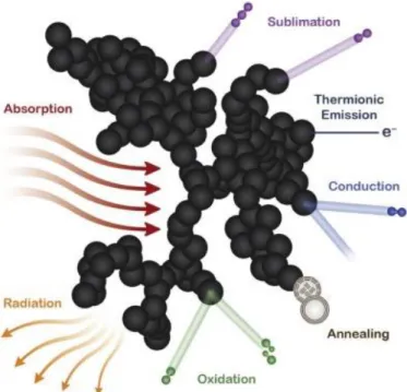
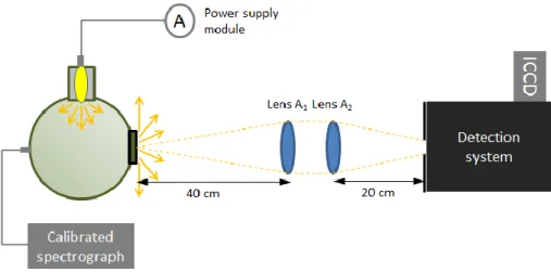
(13) Thèse de Thi Linh Dan Ngo, Université de Lille, 2019. List of figure Figure 1.1.1. Aircraft. emissions from International Aviation, 2005 to 2050 (ICAO. Environmental Report 2016 - Aviation and Climate Change 2017) .................................................... 24 Figure 1.2.1. Structural isomers of butanol ............................................................................................. 28 Figure 1.2.2. Schematic of biobutanol production process. Adapted from (Trindade and Santos 2017) ............................................................................................................................................................. 29 Figure 1.3.1. Emissions from a typical two-engine jet aircraft during 1-hour flight with 150 passengers (ICAO Environmental Report 2016 - Aviation and Climate Change 2017)................... 35 Figure 1.3.2. Schematic diagram of the HEFA process ......................................................................... 38 Figure 2.1.1. Sketch of the burner generating swirled jet flame in this study. .................................. 44 Figure 2.1.2. Specifications of nebulizer DIHEN 170-AA (PhD thesis Lemaire, 2012) ..................... 45 Figure 2.1.3. Sketch design of honeycomb and swirler ........................................................................ 45 Figure 2.1.4. Picture of burner system endorsed in a polycarbonate cage, and mounted on a translation stage, below the extraction system and the detector. This experimental configuration is used for LII/LIF measurement.............................................................................................................. 46 Figure 2.1.5. Photo (left) and schematic (right)f of MiniCAST burner (model 5201 C).................... 47 Figure 2.1.6. Photo and schematic of Liquid JING CAST (Private communication, Irimiea, 2019) 48 Figure 2.3.1. Scheme of extraction system .............................................................................................. 49 Figure 2.3.2. Sampling system of Front/Back filters .............................................................................. 50 Figure 2.4.1. Scheme of the experimental setup used for LII/LIF measurements. ............................ 51 Figure 2.4.2. Perrin-Jablonski diagram representing energy levels and spectra (Valeur 2005). ISC is intersystem crossing. IC is internal conversion ................................................................................. 52 Figure 2.4.3. Illustration of processes influencing the temperature and mass of a particle during LII-signal collection (Michelsen et al. 2015)............................................................................................ 54 Figure 2.4.4. Top-hat spatial profile for 1064 nm laser irradiation (1127.5 µm x 1105.5 µm, ellipticity 98.0%) ......................................................................................................................................... 59 Figure 2.4.5. Top-hat spatial profile for 532 nm laser irradiation (1265 µm x 1248 µm, ellipticity 97.7%) ........................................................................................................................................................... 59 Figure 2.4.6. Working principle of a photomultiplier tube .................................................................. 60 Figure 2.4.7. Scheme of working principle of an ICCD intensifier ..................................................... 61 Figure 2.4.8. Set up used to determine the optical response of measurement system ..................... 62 Figure 2.5.1. Scheme of working principle of L2MS technique (Irimiea 2017). ................................. 63 Figure 2.5.2. Cross section of analysis chamber, top view (Irimiea 2017). ......................................... 64 Figure 2.5.3. Optical pathway of the laser desorption beam. .............................................................. 64 Figure 2.5.4. Optical pathway of the ionization laser beam. ................................................................ 65 Figure 2.5.5. Photo ionization mechanisms for molecular species commonly involved in combustion chemistry (Desgroux, Mercier, and Thomson 2013) ....................................................... 66 Figure 2.5.6. Ion path in the ToF-MS, from the generation of the ion packets in the analysis chamber to their detection by the micro channel plate detector (Irimiea 2017). ............................... 67. 13 © 2019 Tous droits réservés.. lilliad.univ-lille.fr.

(14) Thèse de Thi Linh Dan Ngo, Université de Lille, 2019. Figure 2.5.7. (a) A ToF-SIMS instrument with component labeled, including (A) the ToF-MS, (B, C) ion sources for sputtering and analysis, and (D) load lock for introducing samples. (b) Schematic presentation of some of the internal components of a ToF-SIMS instrument. The primary ions are represented in yellow, while secondary ions are represented with blue (Cushman et al. 2018) ................................................................................................................................ 67 Figure 2.5.8. Scheme of working principle of SIMS. ............................................................................. 68 Figure 3.1.1. Theoretical collection efficiencies of particles collection mechanisms for a fibrous filter 1mm thick with 2m fibers and an air velocity of 10 cm/s. Total shows the collection efficiency of the filter due to all mechanisms combined (Lindsley 2016). ......................................... 75 Figure 3.1.2. Photos of CAST front and back samples .......................................................................... 76 Figure 3.2.1. L2MS mass spectra of CAST samples ............................................................................... 77 Figure 3.2.2. Score plot of PC1 and PC2 from PCA analyses applied of L2MS mass spectra of CAST samples............................................................................................................................................. 79 Figure 3.2.3. Loadings corresponding to PC1 and PC2 presented in Figure 3.2.2 ............................ 79 Figure 3.3.1. Positive SIMS mass spectra of CAST samples ................................................................. 80 Figure 3.3.2. Total PAH content detected with SIMS on CAST front and back samples. Red and grey dots represent OC/TC ratios measured in previous studies on the same set points of CAST. ...................................................................................................................................................................... 81 Figure 3.3.3. Score plot of PCA applied on positive SIMS spectra of CAST samples ...................... 82 Figure 3.3.4. Loadings corresponding to PC1 and PC2 components in the PCA of positive polarity SIMS spectra of CAST samples ................................................................................................................ 82 Figure 3.3.5. Negative SIMS mass spectra of CAST samples ............................................................... 83 Figure 3.3.6. Score plot of PCA applied on negative SIMS spectra of CAST front and back samples ...................................................................................................................................................................... 84 Figure 3.3.7. Loadings corresponding to PC1 and PC2 presented in Figure 3.3.6 ............................ 84 Figure 3.3.8. Variation of the content of various markers, derived from negative SIMS mass spectra .......................................................................................................................................................... 85 Figure 4.1.1. Fluence curves obtained at 152 cm HAB in the diesel flame with (a) 266 nm and (b) 532 nm excitation wavelength. Detection wavelength ranges are 700-892 nm and 700-800 nm, respectively. ................................................................................................................................................ 88 Figure 4.1.2. Photo of diesel swirled jet flame and its 2D plots of soot and soot precursor obtained by coupling of LII and LIF at 266, 532 and 1064 nm excitation. .......................................................... 90 Figure 4.1.3. Left: LIF profile obtained at the centerline of diesel flame with 266 nm excitation. Right: LIF spectra with 266 nm excitation at different HABs in diesel flame (obtained at the centerline). Laser fluence used is 1.5 mJ/cm2. Detection wavelength range is 295-564 nm. ........... 91 Figure 4.1.4. Comparison of normalized LIF spectra obtained with pure diesel in quartz cuvette and LIF spectra of several HABs in diesel flame, measured with 266 nm excitation. ..................... 92 Figure 4.1.5. Normalized LIF spectra obtained at the centerline of diesel flame with 266 nm excitation. .................................................................................................................................................... 93. 14 © 2019 Tous droits réservés.. lilliad.univ-lille.fr.

(15) Thèse de Thi Linh Dan Ngo, Université de Lille, 2019. Figure 4.1.6. Left: LIF profile obtained at the centerline of the diesel flame with 532 nm excitation. Right: LIF spectra with 532 nm excitation at different HABs in the diesel flame (obtained at the centerline). Laser fluence used is 6.3 mJ/cm2.......................................................................................... 93 Figure 4.1.7. Normalized LIF spectra obtained at the centerline of the diesel flame with 532 nm excitation. .................................................................................................................................................... 94 Figure 4.1.8. LII profile obtained at the centerline of diesel flame with 532 nm laser excitation. The measurement is conducted with a laser fluence of 180.6 mJ/cm2. Detection wavelength range is 750-882 nm. ................................................................................................................................................. 95 Figure 4.1.9. LII temporal profile obtained at different HABs with 532 nm laser excitation. The decay curves are averaged over 1000 laser pulses. The detection wavelength is centered at 900 nm with a width range of 6 nm................................................................................................................ 96 Figure 4.1.10. Normalized LII signal at 186 mm HAB in the diesel flame ......................................... 97 Figure 4.1.11. Time constant obtained from the temporal LII profile in Figure 4.1.9 ....................... 97 Figure 4.1.12. LII profile obtained at the centerline of the diesel flame with 1064 nm laser excitation. The detection wavelength is 535-803 nm. ............................................................................ 98 Figure 4.1.13. LII temporal profile obtained at different HABs with 1064 nm laser excitation. The decay curves are averaged over 1000 laser pulses. ............................................................................... 98 Figure 4.1.14. Time constant corresponding to the LII signal presented in Figure 4.1.13 (1064 nm excitation), compared with time constant obtained with 532 nm excitation ..................................... 99 Figure 4.1.15. Variation of soot particles and their precursors in the centerline of the diesel flame. Blue and pink areas show the potential zones of two different classes of species, which correspond to the 1st and 2nd peaks of Vis-LIF profile obtained with 532 nm excitation wavelength. ................................................................................................................................................. 99 Figure 4.1.16. Photo of n-butanol swirled jet flame and its 2D plots of soot and soot precursor obtained by coupling of LII and LIF at 266, 532 and 1064 nm excitation. ........................................ 101 Figure 4.1.17. LIF fluence curve (in linear-log (left) and linear-log (right) graphs) obtained with 266 nm wavelength excitation at 70 mm HAB in n-butanol flame. Emitted light is collected in the spectral range 295 - 470 nm..................................................................................................................... 102 Figure 4.1.18. Left: LIF profile obtained at the centerline of n-butanol flame with 266 nm excitation. Right: LIF spectra with 266 nm excitation at different HABs in n-butanol flame (obtained at the centerline). Laser fluence used is 42.13 mJ/cm2. ...................................................... 103 Figure 4.1.19. Normalized fluorescence emissions of n-butanol cold droplets, obtained with 266 nm excitation ............................................................................................................................................ 103 Figure 4.1.20. Normalized LIF spectra obtained at the centerline of n-butanol flame with 266 nm excitation. .................................................................................................................................................. 104 Figure 4.1.21. Laser induced incandescence (LII) fluence curve obtained with 266 nm wavelength excitation at 185 mm HAB in n-butanol flame. Emitted light is collected in the spectral range 800 900 nm........................................................................................................................................................ 105 Figure 4.1.22. Left: LIF profile obtained at the centerline of n-butanol flame with 532 nm excitation. Right: LIF spectra with 532 nm excitation at different HABs in n-butanol flame (obtained at the centerline). Laser fluence used is 10.73 mJ/cm2 ....................................................... 106 15 © 2019 Tous droits réservés.. lilliad.univ-lille.fr.

(16) Thèse de Thi Linh Dan Ngo, Université de Lille, 2019. Figure 4.1.23. Normalized LIF spectra obtained at the centerline of n-butanol flame with 532 nm excitation ................................................................................................................................................... 106 Figure 4.1.24. LII fluence curve obtained with 1064 nm wavelength excitation at 196 mm HAB in n-butanol flame. Emitted light is collected in the spectral range 700 - 800 nm. .............................. 107 Figure 4.1.25. LII profile obtained at the centerline of n-butanol flame with 1064 nm laser excitation. Laser fluence is used at 439.2 mJ/cm2 ................................................................................. 108 Figure 4.1.26. LII temporal profile obtained at different HABs in n-butanol flame with 1064 nm laser excitation. The decay curves are averaged over 1000 laser pulses. Laser fluence is 344.23 mJ/cm2. ....................................................................................................................................................... 108 Figure 4.1.27. Variation of soot particles and their precursors in the centerline of n-butanol flame .................................................................................................................................................................... 109 Figure 4.1.28. Photo of mixture swirled jet flame and its 2D plots of soot and soot precursor obtained by coupling of LII and LIF at 266, 532 and 1064 nm excitation......................................... 110 Figure 4.1.29. Left: LIF profile obtained at the centerline of the mixture flame with 266 nm excitation. Right: LIF spectra with 266 nm excitation at different HABs in the mixture flame (obtained at the centerline). Laser fluence used is 1.1 mJ/cm2. .......................................................... 111 Figure 4.1.30. Comparison of LIF spectra obtained at certain HABs in the mixture flame and on cold droplets of mixture fuel .................................................................................................................. 111 Figure 4.1.31. Normalized LIF spectra obtained at the centerline of mixture flame with 266 nm excitation. .................................................................................................................................................. 112 Figure 4.1.32. Left: LIF profile obtained at the centerline of the mixture flame with 532 nm excitation. Right: LIF spectra with 532 nm excitation at different HABs in the mixture flame (obtained at the centerline). Laser fluence used is 6.3 mJ/cm2. .......................................................... 113 Figure 4.1.33. Normalized LIF spectra obtained at the centerline of the mixture flame with 532 nm excitation. ........................................................................................................................................... 114 Figure 4.1.34. LII profile obtained at the centerline of the mixture flame with 532 nm laser excitation. Laser fluence is used at 179.8 mJ/cm2 ................................................................................. 114 Figure 4.1.35. LII temporal profile obtained at different HABs with 532 nm laser excitation. The decay curves are averaged over 1000 laser pulses. ............................................................................. 115 Figure 4.1.36. Evolution of LII time constant (obtained from the temporal profiles in Figure 4.1.35) with the HAB................................................................................................................................ 115 Figure 4.1.37. LII profile obtained at the centerline of the mixture flame with 1064 nm laser excitation. Laser fluence is 340.1 mJ/cm2............................................................................................... 116 Figure 4.1.38. LII temporal profile obtained at different HABs in the mixture flame with 1064 nm laser excitation. The decay curves are averaged over 1000 laser pulses. ......................................... 116 Figure 4.1.39. Time constant corresponding to the LII signal presented in Figure 4.1.38 (1064 nm excitation), compared with time constant obtained with 532 nm excitation ................................... 117 Figure 4.1.40. Variation of soot particles and their precursors in the centerline of the mixture flame. Blue and pink areas show the potential zones of two different classes of species corresponding to the Vis-LIF profile obtained with 532 nm excitation wavelength. ..................... 117. 16 © 2019 Tous droits réservés.. lilliad.univ-lille.fr.

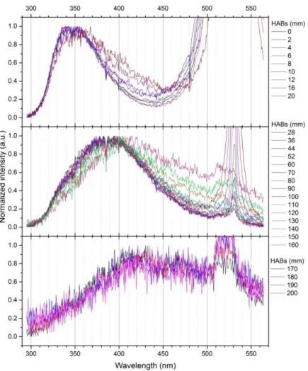
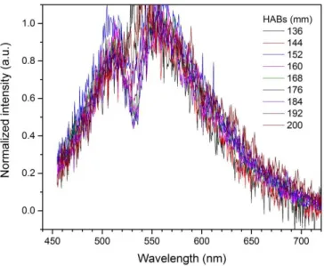
(17) Thèse de Thi Linh Dan Ngo, Université de Lille, 2019. Figure 4.1.41. 2D plots of soot and soot precursors obtained by coupling of LII and LIF at 266 and 532 nm excitation taken in Jet A-1 swirled jet flame. .......................................................................... 118 Figure 4.1.42. Left: LIF profile obtained at the centerline of Jet A-1 flame with 266 nm excitation. Right: LIF spectra with 266 nm excitation at different HABs in Jet A-1 flame (obtained at the centerline). Laser fluence used is 1.4 mJ/cm2........................................................................................ 119 Figure 4.1.43. Comparison of LIF spectra taken at several HABs and cold droplets of Jet A-1 fuel, with 266 nm excitation ........................................................................................................................... 120 Figure 4.1.44. Normalized LIF spectra obtained at the centerline of Jet A-1 flame, with 266 nm excitation ................................................................................................................................................... 121 Figure 4.1.45. Left: LIF profile obtained at the centerline of Jet A-1 flame with 532 nm excitation. Right: LIF spectra with 532 nm excitation at different HABs in the Jet A-1 flame (obtained at the centerline). Laser fluence used is 5.8 mJ/cm2. ...................................................................................... 122 Figure 4.1.46. Normalized LIF spectra obtained at the centerline of Jet A-1 flame, with 532 nm excitation ................................................................................................................................................... 123 Figure 4.1.47. LII profile obtained at the centerline of the Jet A-1 flame with 532 nm excitation. The signal is integrated in the 750 – 883 nm spectral range. Laser fluence used is 183.1 mJ/cm2. 123 Figure 4.1.48. LII temporal profile obtained at different HABs in the Jet A-1 flame with 532 nm laser excitation. The decay curves are averaged over 1000 laser pulses. ......................................... 124 Figure 4.1.49. Time constant calculated from the decay curves in Figure 4.1.48 ............................ 124 Figure 4.1.50. Variation of soot particles and their precursors in the centerline of the Jet A-1 flame........................................................................................................................................................... 125 Figure 4.1.51. 2D plots of soot and soot precursors obtained by coupling of LII and LIF at 266 and 532 nm excitation taken in the SPK swirled jet flame. ........................................................................ 126 Figure 4.1.52. Left: LIF profile obtained at the centerline of the SPK flame with 266 nm excitation. Right: LIF spectra with 532 nm excitation at different HABs in the SPK flame (obtained at the centerline). Laser fluence used is 1.5 mJ/cm2........................................................................................ 126 Figure 4.1.53. Comparison of LIF emission from several HABs in the SPK flame and from SPK droplets ...................................................................................................................................................... 127 Figure 4.1.54. Normalized spectra of fluorescence emissions at different HABs in the SPK flame, obtained with 266 nm excitation. ........................................................................................................... 128 Figure 4.1.55. Left: LIF profile obtained at the centerline of the SPK flame with 532 nm excitation. Right: LIF spectra with 532 nm excitation at different HABs in the SPK flame (obtained at the centerline). Laser fluence used is 5.8 mJ/cm2........................................................................................ 129 Figure 4.1.56. Normalized LIF spectra obtained at the centerline of the SPK flame with 532 nm excitation. .................................................................................................................................................. 129 Figure 4.1.57. LII profile obtained at the centerline of the SPK flame with 532 nm excitation. Emitted light is collected in the range 750 - 883 nm. ........................................................................... 130 Figure 4.1.58. Decay curves of LII signal taken in the sooting zone of the SPK flame. Each curve is recorded with 1000 laser pulses. ............................................................................................................ 130 Figure 4.1.59. Time constant calculated from Figure 4.1.58 ............................................................... 131. 17 © 2019 Tous droits réservés.. lilliad.univ-lille.fr.

(18) Thèse de Thi Linh Dan Ngo, Université de Lille, 2019. Figure 4.1.60. Variation of soot particles and their precursors detected from LII/LIF measurements in the centerline of the SPK flame. .............................................................................. 131 Figure 4.1.61. Representation of the slope of three LII spectra from (a) Diesel 156 mm HAB, (b) Mixture 172 mm HAB and (c) N-butanol 200 mm HAB. From the slope, the soot average temperature be deduced. The LII signal is obtained with 1064 nm excitation................................ 133 Figure 4.1.62. Schematic of the optical set up for the calibration with the sphere .......................... 134 Figure 4.1.63. 2D profile of soot volume fraction in three flames: diesel, mixture and n-butanol 137 Figure 4.1.64. 2D profile of soot volume fraction in three flames: Jet A-1 and SPK ....................... 138 Figure 4.1.65. Average soot volume fraction of three automobile-fueled flames (left panel) and two aero-fueled flames (right panel). Error bars represent the variation of E(m) in function of the maturity of soot particles. ....................................................................................................................... 138 Figure 4.2.1. Photos of the diesel flame and Front and Back filters corresponding to different HABs. (The photo of flame is 90o rotated to have better vision) ....................................................... 139 Figure 4.2.2. L2MS mass spectra of front diesel samples at different HABs. 266 nm is used for ionization. .................................................................................................................................................. 142 Figure 4.2.3. L2MS mass spectra of back diesel samples at different HABs. 266 nm is used for ionization. .................................................................................................................................................. 143 Figure 4.2.4. H/C diagram from L2MS mass spectra of the combustion products collected on Front filters at different HABs in the diesel flame. Black dots represent odd numbers of C, red dots represent even numbers of C. The blue lines represent the limits of benzene oligomers and the red lines represent pericondensed PAHs (D’Anna, Sirignano, and Kent 2010). The green lines represent alkyl-phenathrene series........................................................................................................ 144 Figure 4.2.5. Score plots of PC1, PC2 and PC3 of PCA results obtained on L2MS mass spectra of diesel samples ........................................................................................................................................... 146 Figure 4.2.6. Loadings corresponding to PC1, PC2 and PC3 presented in Figure 4.2.5................. 146 Figure 4.2.7. Positive SIMS mass spectra of diesel front and back samples. Data is normalized by the total ion count of each spectrum. .................................................................................................... 148 Figure 4.2.8. Negative SIMS mass spectra of diesel front samples. The spectra are normalized to the total ion count .................................................................................................................................... 150 Figure 4.2.9. SIMS spectra (negative polarity) of diesel back samples ............................................. 151 Figure 4.2.10. Score plots of PC1, PC2 and PC3 of PCA applied on SIMS mass spectra (positive polarity) of diesel samples ...................................................................................................................... 152 Figure 4.2.11. Loadings of PC1, PC2 and PC3 corresponding to Figure 4.2.10 ............................... 153 Figure 4.2.12. Score plot of PC1 and PC2 applied on negative SIMS spectra of diesel samples ... 154 Figure 4.2.13. Loading plots corresponding to PC1 and PC2 shown in Figure 4.2.12 ................... 155 Figure 4.2.14. Photos of n-butanol flame and Front and Back filters corresponding to different HABs. (The photo of the flame is rotated 90o for better view)........................................................... 155 Figure 4.2.15. L2MS mass spectra of n-butanol front samples, obtained with 532 nm laser desorption and 266 nm laser ionization ................................................................................................ 157 Figure 4.2.16. L2MS mass spectra of n-butanol back samples, obtained with 532 nm laser desorption and 266 nm laser ionization ................................................................................................ 158 18 © 2019 Tous droits réservés.. lilliad.univ-lille.fr.

(19) Thèse de Thi Linh Dan Ngo, Université de Lille, 2019. Figure 4.2.17. Positive SIMS spectra of n-butanol samples. Data is normalized to the total ion count for each spectrum. ......................................................................................................................... 160 Figure 4.2.18. Score plot of PC1 and PC2 applied on positive SIMS mass spectra of n-butanol samples. ..................................................................................................................................................... 161 Figure 4.2.19. Loadings corresponding to PC1 and PC2 as presented in Figure 4.2.18 ................. 162 Figure 4.2.20. Negative SIMS spectra of n-butanol front samples .................................................... 163 Figure 4.2.21. Score plot of PC1 and PC2 for negative SIMS mass spectra of n-butanol samples.164 Figure 4.2.22. Loading plot corresponding to PC1 and PC2 represented in Figure 4.2.21 ............ 165 Figure 4.2.23. Photo of front and back samples collected at 6 HABs in the mixture flame. .......... 165 Figure 4.2.24. L2MS mass spectra of the mixture flame front samples ............................................ 166 Figure 4.2.25. L2MS mass spectra of the mixture flame back samples ............................................. 167 Figure 4.2.26. Score plot of PC1 and PC2 obtained from L2MS mass spectra of the mixture flame front and back samples. .......................................................................................................................... 168 Figure 4.2.27. Loadings corresponding to PC1 and PC2 represented in Figure 4.2.26 .................. 168 Figure 4.2.28. Positive SIMS spectra of the mixture flame front samples ........................................ 169 Figure 4.2.29. Score plot of the two first principal components in PCA applied on positive SIMS spectra of the mixture flame front and back samples. ........................................................................ 170 Figure 4.2.30. Loadings corresponding to PC1 and PC2 presented in Figure 4.2.29 ...................... 170 Figure 4.2.31. Negative SIMS mass spectra of the mixture flame front samples ............................ 172 Figure 4.2.32. Score plot of PC1 and PC2 from PCA analysis applied on negative SIMS mass spectra of the mixture flame samples.................................................................................................... 173 Figure 4.2.33. Loadings corresponding to PC1 and PC2 presented in Figure 4.2.32 ...................... 173 Figure 4.3.1. Temperature measured in the centerline of the three flames with a K-type thermocouple in non-sooting zone ........................................................................................................ 174 Figure 4.4.1. Comparison between the total PAH peak area obtained from L2MS mass spectra and the Vis-LIF signal of the three flames: (a) diesel, (b) n-butanol and (c) mixture. GaussAmp fit is applied for the mixture flame since there are only five HABs sampled for L2MS analysis. ..... 175 Figure 4.4.2. Clustering dendrogram obtained for 193 peaks assigned for hydrocarbon fragments and compounds from SIMS positive spectra of diesel, n-butanol and mixture flame samples. Three clusters are divided within 193 peaks. The peak lists of three clusters are presented in three tables in the figure.................................................................................................................................... 177 Figure 4.4.3. Comparison between the sum of Cluster 3 peak areas normalized to PIC obtained from SIMS positive mass spectra and Vis-LIF signal of the three flames: diesel, n-butanol and mixture....................................................................................................................................................... 178 Figure 4.4.4. Correlation coefficients between in-situ LII/LIF signal recorded for the diesel flame and the. ,. ions defected by SIMS from the diesel flame front samples ........................ 179. Figure 4.4.5. Evolution of. peak area normalized to TIC from SIMS negative mass spectra, in. comparison with IR-LII of (a) diesel and (b) mixture flames............................................................. 180 Figure 4.4.6. Correlation coefficients between in-situ LII/LIF signal and Cn-, CnH- obtained in negative polarity of SIMS mass spectra from n-butanol front samples ........................................... 181. 19 © 2019 Tous droits réservés.. lilliad.univ-lille.fr.

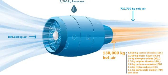
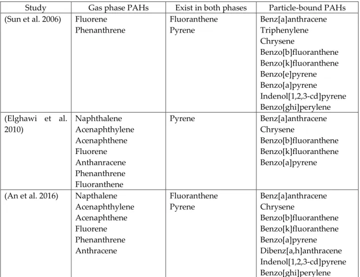
(20) Thèse de Thi Linh Dan Ngo, Université de Lille, 2019. Figure 4.4.7. Evolution of the sum of. ,. and. normalized to TIC from SIMS. negative mass spectra, in comparison with Vis-LIF signal from the three flames. The evolution of C2-/TIC in SIMS mass spectra of n-butanol is also presented............................................................. 182 Figure 4.4.8. Class A and B species defined according to the normalized UV-LIF spectra obtained at the centerline of the diesel flame ....................................................................................................... 183 Figure 4.4.9. Class C and D species defined according to the normalized Vis-LIF spectra obtained at the centerline of the diesel flame ....................................................................................................... 183 Figure 4.4.10. Positions of the five classes detected in the diesel flame. The red and blue dot lines are presumed and extended from the Vis-LIF profile. ....................................................................... 184 Figure 4.4.11. Proposing kinetic pathway of the soot formation in the diesel flame ..................... 186 Figure 4.4.12. Positions and characteristics of the classes of species detected in the n-butanol flame........................................................................................................................................................... 187 Figure 4.4.13. Class A and B species defined according to the normalized UV-LIF spectra obtained at the centerline of the n-butanol flame ................................................................................ 188 Figure 4.4.14. Normalized LIF spectra obtained at the centerline of the n-butanol flame with 532 nm excitation ............................................................................................................................................ 189 Figure 4.4.15. Proposing kinetic pathway of the soot formation in the n-butanol flame............... 189 Figure 4.5.1. Comparison of Vis-LIF signal and average soot volume fraction (calculated from the LII signal) for the three flames: diesel, mixture and n-butanol. ........................................................ 190 Figure 4.5.2. C-H or O-H (black) and C-C or C-O (red) bond dissociation energies (BDEs) (kcal mol-1) for n-butanol. Numbers in parentheses ( ) represent the difference in BDEs with respect to a primary C-H bond. Numbers in brackets [ ] are experimental values (Pelucchi et al. 2016). .... 190 Figure 4.5.3. Comparison of Vis-LIF signal and average soot volume fraction (calculated from LII signal) for the Jet A-1 and SPK flames. ................................................................................................. 192 Figure 4.5.4. Vis-LIF spectra of five flames: diesel, mixture, n-butanol, Jet A-1 and SPK. The spectra are normalized to their maximum intensity. .......................................................................... 193 Figure 5.1.1. Schematic of the experiment on liquid CAST and sampling line used for the analysis of emissions produced after the combustion of standard and alternative jet fuels ........................ 196 Figure 5.1.2. Photo of the experimental set up ..................................................................................... 197 Figure 5.2.1. Fluence curves obtained for 105 L min-1 Jet A-1 fuel and 105 L min-1 SPK fuel burned with 2, 2.5 and 3 L/min oxidation air flow. The fluence curves are obtained in the exhaust of the CAST without CS. Left panel shows the original fluence curves whereas right panel shows the fluence curves normalized to the maximum point of each curve. ............................................. 199 Figure 5.2.2. Comparison of the fluence curves obtained with and without CS treatment from Jet A-1 and SPK fuels. ................................................................................................................................... 199 Figure 5.2.3. Fluence curves obtained for 105 L min-1 Jet A-1 fuel burned with 2, 2.5, 3 L/min oxidation air flow. Each graph corresponds to one setting of the oxidation flow. Black and red line-scatters represent results obtained in the exhaust of CAST without CS and with CS, respectively. .............................................................................................................................................. 200 Figure 5.2.4. Fluence curves obtained for 105 L min-1 SPK fuel burned with 2, 2.5, 3 L/min oxidation air flow. Each graph corresponds to one setting of the oxidation flow. Blue and orange 20 © 2019 Tous droits réservés.. lilliad.univ-lille.fr.

(21) Thèse de Thi Linh Dan Ngo, Université de Lille, 2019. line-scatters represent results obtained in the exhaust of CAST without CS and with CS, respectively. .............................................................................................................................................. 200 Figure 5.3.1. Photos of front and back samples collected at different set points with the ‚liquid‛ CAST .......................................................................................................................................................... 201 Figure 5.3.2. L2MS mass spectra of front samples collected in the CAST exhaust using Jet A-1 as fuel with three different oxidation air flow rates (upper panels: 2 L/min; middle panels: 2.5 L/min; lower panels: 3 L/min). The exhaust is treated with CS (right panels) or without CS (raw – left panels). ................................................................................................................................................ 202 Figure 5.3.3. L2MS mass spectra of front samples collected in the CAST exhaust using SPK as fuel with three different oxidation air flow rates (upper panels: 2 L/min; middle panels: 2.5 L/min; lower panels: 3 L/min). The exhaust is treated with CS (right panels) or without CS (raw – left panels)........................................................................................................................................................ 203 Figure 5.3.4. L2MS mass spectra of front samples collected in the CAST exhaust using S50 as fuel with three different oxidation air flow rates (upper panels: 2 L/min; middle panels: 2.5 L/min; lower panels: 3 L/min). The exhaust is treated with CS (right panels) or without CS (raw – left panels)........................................................................................................................................................ 204 Figure 5.3.5. Average m/z detected in L2MS mass spectra of liquid CAST front samples ............ 205 Figure 5.3.6. Clustering dendrogram obtained with L2MS mass spectra of liquid CAST front samples ...................................................................................................................................................... 205 Figure 5.3.7. PCA score plot (left panel) obtained from L2MS mass spectra of liquid CAST front samples and loadings (right panel) of first two principal components ........................................... 206 Figure 5.3.8. Score and loading plots of PCA applied on L2MS mass spectra of liquid CAST front raw samples .............................................................................................................................................. 207 Figure 5.3.9. Variation of alkyl-PAHs sum, normalized to TIC, detected in L2MS spectra of liquid CAST front raw samples ......................................................................................................................... 207 Figure 5.3.10. L2MS mass spectra of back samples collected in the CAST exhaust using Jet A-1 as fuel with three different oxidation air flow rates (upper panels: 2 L/min; middle panels: 2.5 L/min; lower panels: 3 L/min). The exhaust is treated with CS (right panels) or without CS (raw – left panels). ................................................................................................................................................ 208 Figure 5.3.11. L2MS mass spectra of back samples collected in the CAST exhaust using SPK as fuel with three different oxidation air flow rates (upper panels: 2 L/min; middle panels: 2.5 L/min; lower panels: 3 L/min). The exhaust is treated with CS (right panels) or without CS (raw – left panels). ................................................................................................................................................ 209 Figure 5.3.12. L2MS mass spectra of back samples collected in the CAST exhaust using SPK as fuel with three different oxidation air flow rates (upper panels: 2 L/min; middle panels: 2.5 L/min; lower panels: 3 L/min). The exhaust is treated with CS (right panels) or without CS (raw – left panels). ................................................................................................................................................ 209 Figure 5.3.13. Positive SIMS mass spectra of front samples collected in the CAST exhaust using Jet A-1, SPK and S50 as fuel with 2.5 L/min oxidation air flow rate. ................................................ 210 Figure 5.3.14. Negative SIMS mass spectra of front samples collected in the CAST exhaust using Jet A-1, SPK and S50 as fuel with 2.5 L/min oxidation air flow rate. ................................................ 211 21 © 2019 Tous droits réservés.. lilliad.univ-lille.fr.

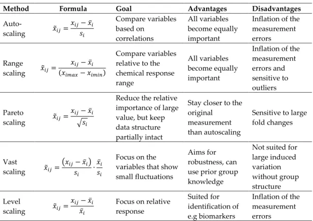
(22) Thèse de Thi Linh Dan Ngo, Université de Lille, 2019. Figure 5.3.15. Score plot of PCA applied on positive SIMS mass spectra of liquid CAST samples .................................................................................................................................................................... 212 Figure 5.3.16. Loadings corresponding to PC1 and PC2 displayed in Figure 5.3.15 ...................... 212 Figure 5.3.17. PCA applied on negative SIMS spectra of liquid CAST samples ............................. 213 Figure 5.3.18. Coefficients corresponding to PC1 and PC2 presented in Figure 5.3.17 ................. 213 Figure 5.3.19. Variation of total PAH peaks area in positive SIMS mass spectra and total CnHpeak area in negative SIMS mass spectra obtained with Jet A-1, S50 and SPK burned with 2.5L/min oxidation flow. ......................................................................................................................... 214. List of tables Table 1.2.1. Properties of diesel and certain potential biofuels ........................................................... 28 Table 1.2.2. Literature review on soot emissions of combustion involving n-butanol..................... 31 Table 1.3.1. Conversion processes approved as annexes to ATSM D7566 (Status of Technical Certification of Aviation Alternative Fuels 2017) .................................................................................. 36 Table 1.3.2. Literature review on soot emissions of combustion involving HEFA-SPK .................. 39 Table 2.1.1. Flow rates of fuels, nebulization nitrogen and oxidation air in five swirled flames .. 47 Table 2.5.1. Overview of widely-used PCA scaling method. The mean is calculated as and the standard deviation is calculated as. ................................... 70. Table 3.1.1. Experimental conditions corresponding to the four studied set points ........................ 74 Table 3.2.1. List of PAHs present in gas phase and particle-bound phase in some studies. ........... 78 Table 4.1.1. Configuration of LII/LIF measurements carried out on five swirled flames. ............... 89 Table 4.4.1. Literature on. and. as indicators for EC and OC ........................................ 179. Table 4.4.2. Characteristics of four classes of species detected in the diesel flame ......................... 184 Table 4.4.3. Comparison between the total PAH peak area obtained from L2MS mass spectra and the Vis-LIF signal of the three flames: (a) diesel, (b) n-butanol and (c) mixture. GaussAmp fit is applied for the mixture flame since there are only five HABs sampled for L2MS analysis.......... 185 Table 5.1.1. Properties of Jet A-1 and SPK used in the experiment................................................... 197. 22 © 2019 Tous droits réservés.. lilliad.univ-lille.fr.

(23) Thèse de Thi Linh Dan Ngo, Université de Lille, 2019. Chapter 1. Introduction. 23 © 2019 Tous droits réservés.. lilliad.univ-lille.fr.

(24) Thèse de Thi Linh Dan Ngo, Université de Lille, 2019. 1. Introduction 1.1. General More than 90% of primary consumption of energy in the world is used in the combustion (Tissot 2003). The demand of worldwide energy, especially fossil energy, has been increased with the development of technology and civilization. Petroleum fuels – a type of fossil combustibles – are actually being used in important quantity in transport system. However, there are two big problems caused by the utilization of fossil fuels: (1) the shortage of their stocks because they are not renewable and (2) the increase of the concentration of carbon dioxide in the atmosphere due to their combustion. In lately decades, the extreme increase of greenhouse gas provokes the climate change all around the planet, leading to the more frequent extreme climatic phenomena. Biofuels appears as an interesting and promising solution that is able to solve both problems: decrease the dependence of human on fossil fuels and reduce the negative impact on environment. Biofuels are considered as a renewable energy and could be produced from alimental or non-alimental biomass stocks. The utilization of biofuels as a source of energy would not increase the total concentration of carbon containing in. in the atmosphere because biomass uses the. for their growth due to the photosynthetic process.. Figure 1.1.1. Aircraft emissions from International Aviation, 2005 to 2050 (ICAO Environmental Report 2016 Aviation and Climate Change 2017). Figure 1.1.1 shows the estimated scenario of. emissions in aviation sector from 2020 – 2050. with different options. It can be seen from the figure that biofuels take an important role to achieve the goal of carbon-neutral growth in 2050. In other words, the carbon-neutral growth cannot be without the use of biofuels. However, care must be taken in using biofuels for the combustion. Since the engines have been always designed to use fossil fuels, any modification of fuels could influence many aspects as 24 © 2019 Tous droits réservés.. lilliad.univ-lille.fr.

(25) Thèse de Thi Linh Dan Ngo, Université de Lille, 2019. technical problems (density, viscosity, filtration, volatility,…) or fuel consumption (concerning to calorific values), or the exhaust emissions as. , hydrocarbons (. ), particulate matter (PM),. ,… Most of studies reported that the use of biofuels reduces the emissions of particles, but increases. , soot. emissions (Schumacher et al. 1996; Bünger et al. 2000; Kooter et al.. 2011; Krahl et al. 2002; Dorado 2003). However, some scholars reported that there is an increase of benzene, aldehydes and ozone precursors in the exhaust of biofuels (Geyer, Jacobus, and Lestz 1984; Krahl et al. 2001; Krahl et al. 2002; Turrio-Baldassarri et al. 2004). Jaramillo et al. (2018) stated that the differences in fuels and combustion conditions affect strongly the physicochemical properties of emitted particles. And with these differences, the biological/toxicological responses could be affected. There is inconsistency of this problematic among the studies. A lower mutagenic potency is found due to the lower content of PAHs in exhaust of biodiesel compared to diesel as in the studies of (Bünger et al. 2000; Krahl et al. 2002). Whereas in other studies, a strong increase of cytotoxicity, mutagenicity and genotoxicity of emissions from biofuels (compared to conventional fossil fuels) is reported (Topinka et al. 2012; Kooter et al. 2011; Bünger et al. 2007). Among different types of species in the exhaust emissions of the combustion, we are interested mostly in soot emissions and polycyclic aromatic compounds. These unwanted byproducts are the result of incomplete combustion. These emissions classify as negative role players in the climate and environment. In the atmosphere, these particles can play as condensation nuclei forming cloud, which have a cooling effect on Earth’s atmosphere or they can absorb sun radiation and produce the greenhouse effect. This particulate matter could be the second largest contributor to global warming (Jacobson 2001; Ramanathan and Carmichael 2008). The deposition of them on snow is considered as a major source for arctic sea ice retreat and melting glaciers (de_Richter and Caillol 2011). The size of particles covers many orders of magnitude. They are classified in function of their aerodynamic diameter as PM10 (< 10 m), PM2.5, PM1 and UFP (ultra-fine PM, < 100 nm). The smallest particles are the most dangerous ones because they are considered to exacerbate respiratory, cardiovascular, and allergic diseases due to their small respirable size, large surface area, surface reactivity and potential toxicity (Shiraiwa, Selzle, and Pöschl 2012; Libalova et al. 2016; Zhang and Balasubramanian 2017). The PAHs carried along with soot particles in exhaust emissions of combustion have been reported to cause impaired lung function in asthmatics and thrombotic effects in short-term. In long term, several PAHs are identified as highly toxic, mutagenic and/or carcinogenic to microorganisms as well as higher systems including humans (Kim et al. 2013; Abdel-Shafy and Mansour 2016; Shiraiwa, Selzle, and Pöschl 2012). Therefore it is necessary to investigate soot and PAH emissions in the exhaust of different fuels. Soot is the terms used for particulate matter resulting from incomplete combustion of organic materials. In literature, there are many other terms used as Black Carbon (BC), Black carbon (CB), Refractory Black Carbon (rBC), Equivalent Black Carbon (eBC), Total Carbon (TC), Brown Carbon (BrC), Light Absorbing Carbon (LAC), Elemental Carbon (EC), Organic Carbon (OC), etc. 25 © 2019 Tous droits réservés.. lilliad.univ-lille.fr.

(26) Thèse de Thi Linh Dan Ngo, Université de Lille, 2019. These terms are used related to specific material properties and/or techniques used to investigate them. This combustion by-product is not a pure compound. It mainly contains amount of. as well as. and a significant. and metals, etc. depending on its origin. Soot is present everywhere. around us, from natural sources as interstellar dust or biomass burning, to anthropogenic sources as transportation, industrial activities or domestic activities. Soot formation is a complex process containing series of mechanisms. The formation starts after the fuel pyrolysis, which produces a significant amount of acetylene ( of. ) in the incipient zone of a flame. The addition. to molecular precursors states under the name of HACA mechanism ( abstraction. addition). This mechanism was first introduced by (Frenklach and Wang 1991). It describes a repetitive reaction pathway involving acetylene molecules in the formation of the first aromatic ring up to large molecules. The nucleation process – which is the initiation of soot particles has not been well understood (Desgroux, Mercier, and Thomson 2013). There are few pathways for this step proposed by scholars. (Homann 1998) suggested a pathway stating the formation of fullerene-like structures by the bimolecular reactions produced between two PAHs, involving coordinate detachment of. or so-called zipper mechanism. (Frenklach 2002) proposed another. pathway which involves the coagulation of PAHs on compact clusters through collisions, due to Van der Waals interactions, forming PAH dimers, trimmers, tetramers and so on. They assumed that the formation of dimers marks the emergence of the ‚solid‛ particle phase. Another mechanism states that the formation of the first nuclei is due to the chemical coalescence of PAHs through. bonds which results in a tridimensional structure (Richter and Howard 2000).. After the first nuclei are formed, the surface of soot particles increases by two processes: the condensation of PAHs onto the soot carbon matrix, and heterogeneous reactions between soot carbonaceous matrix and the surrounding gaseous precursors with HACA mechanism (Frenklach and Wang 1991; Balthasar 2000). The newly formed soot particles are called nascent soot particles. During the particle coagulation process, sticking collisions between particles during the mass growth process significantly increases particles size and decreases particle number without changing the total mass of soot present. This process is accompanied by a progressive reduction of the number of hydrogen and a rearrangement of the internal structure of soot particles which give them the spherical shape. After coagulation, particles can undergo a number of surface reactions having as consequence the aggregation of the particles. During the collision process, mature soot is not coagulating anymore, but particles can merge. At the final step of the process, oxidation of PAHs and soot particles takes place. It decreases the mass of PAHs and soot materials through the formation of. and. (Richter and Howard 2000).. 1.2. N-butanol as alternative for diesel fuel Transport is Europe’s biggest source of carbon emissions, contributing 27% to the EU’s total emission. Transport is the only sector in which emissions have grown since 1990, contributing to the increase in the EU’s overall emissions in 2015 (Todts 2018). Among different fossil fuels that are responsible for the production of greenhouse gases (GHG), diesel is responsible for more than 90% of PM emission according to the study of (Minjares, Wagner, and Akbar 2014). Diesel accounts for more than 40% of global on-road energy consumption and is the main fuel of heavy26 © 2019 Tous droits réservés.. lilliad.univ-lille.fr.