Semi-supervised multi-label feature sélection

B

ADJI

M

OKHTAR

-A

NNABA

U

NIVERSITY

U

NIVERSITE

B

ADJI

M

OKHTAR

-A

NNABA

ﺔ

ـــــ

ﺑﺎﻨﻋ

–

رﺎﺘﺨﻣ ﻲﺟﺎﺑ ﺔﻌﻣﺎﺟ

Faculté des Sciences de L’Ingéniorat Année 2017

Département d’Informatique

THESE

Présentée en vue de l’obtention

du diplôme de Doctorat en Sciences

Semi-Supervised Multi-Label Feature Selection

Option

Intelligence Artificielle

par

M

r

_{Abdelouahid ALALGA}

DEVANT LE JURY

Président :

Mme Labiba SOUICI-MESLATI Professeur Université Badji Mokhtar-Annaba

Directeur de Thèse

Mme Nora TALEB

MCA

Université Badji Mokhtar-Annaba

Co-Directeur de Thèse

Mr Khalid BENABDESLEM

MC, HDR

Université Claude Bernard, Lyon, France

Examinateurs :

Mr Abdelkrim AMIRAT

Professeur Université Med Cherif Messaadia-Souk Ahras

Mr Yacine LAFIFI

Professeur Université 8 Mai 1945- Guelma

Albert Camus

Preface

Acknowledgment

First and foremost, I would like to thank all those who worked so hard to set me obstacle in the road, they showed how far my limits could be pushed and helped me surpass them, without them this work would not have been accomplished. Their e↵orts have reached far beyond this work.

I would like to convey my utmost gratitude to my co-supervisor, mentor and friend Dr. Khalid Benabdeslem, Associate Professor at University of Lyon, for his helpful advice and continued support during my research and writing up. His broad knowledge in the field and his enthusiasm have been of great help to my research study. I am indebted to him for supporting me through my tough times. From the bottom of my heart, I thank him for hosting my internship and his warm welcome at LIRIS. Thanks again for the time we spent talking about every thing and nothing near the co↵ee machine, his down-to-earth attitude serves as a role model for me.

My deep feelings of gratefulness and respect are to Dr. Nora Taleb, Associate Professor at University of Annaba, this work would not have been possible without her unconditional help, encouragements and support. I would also like to express my profound thanks to the members of the Jury. Heartfelt gratitude to Pr. Labiba Souici, Professor at University of Annaba, to have honored me by presiding the jury. I owe my thanks to the Pr. Yacine Lafifi, Professor at University of Guelma, for accepting to take part of the jury as a reviewer. Special thanks go to Pr. Abdelkrim Amirat, Professor at University of Souk-Ahras, for reviewing this thesis. I would also like to extend thanks to my friends, colleagues and anyone who

ii

has contributed with their thoughts and opinions in successfully completing this project.

Last but not least, I would like to acknowledge from the bottom of my heart the endless love and support of my family, specially: my parents, my brothers and sisters. They all kept me going and without them I would not be capable of anything. All I have ever accomplished and I will ever be, I owe to them.

Abstract

N

ever before has there been a time where data is as easy to collect and record as it is now. With the rapid development of digital technologies, data has become both such a precious commodity and a very abundant one. With such abundance, however, come issues related to the quality of the data. Noisy, mean-ingless data has become the bottleneck of machine learning. The most likely source of this noise is due to irrelevant and redundant features. In this regard, feature selection, usually used as a preprocessing step, has become the mainstay of machine learning, especially when dealing with large-scale data. However, feature selection is continuously challenged by new emerging issues. Recently, di↵erent do-main applications suggest data consisting of huge amount of unlabeled instances together with a small number of multi-labeled instances, which we refer to as semi-supervised multi-label learning. On the one hand, multi-labeled data arises in domains where instances are often classified into more than one category. On the other hand, difficulties to obtain such annotated data make it scarce. Multi-label data are hard and coslty to obtain, whereas unMulti-labeled data is abundant. The abundance of this cheap and readily available unlabeled data can make up for the paucity of the annotated ones. Similar to single semi-supervised feature selection, its multi-label counterpart tends to capitalize on unlabeled data to fill the chasm between supervised and unsupervised feature selection.

In the same vein, seeking to address both issues, the present work deals with semi-supervised multi-label feature selection. Based on the premise of data sim-ilarity and the locality of data which we capture through the usage of spectral graph theory, we devised various solutions. More specifically, we firstly study and propose a new filter feature selection framework, that filter out, irrelevant unin-formative features, i.e. features less related to the target concept (encoded by class label information and the geometric structure of the data). We present two transformation-based algorithms plus an algorithm developed based on algorithm adaptation, which is the main contribution of this work (named S-CLS). In ad-dition, we also study the e↵ect of variance on S-CLS and propose a three-fold ensemble learning solution. Finally, we demonstrate the benefits and advantages of our frameworks through various experimental studies. The experiments were carried out on a score of benchmark data sets from various application fields, and

iv

results were promising, showing that our methods either outperform state-of-the-art algorithms or in the worst cases give comparable results.

Keywords: Feature selection, constraints, semi-supervised learning, multi-label classification, spectral graph theory, ensemble methods.

R´

esum´

e

I

l n’y avait jamais eu un temps o`u les donn´ees sont aussi faciles `a collecter et `a enregistrer que maintenant. Avec l’avenement et le d´eveloppement rapide des technologies num´eriques, les donn´ees sont devenues `a la fois un bien pr´ecieux et tr`es abondant. Cependant, avec une telle profusion, se posent des questions relatives `a la qualit´e de ces donn´ees. Des donn´ees bruit´ees et sans un quelconque apport informationnel sont devenues le goulot d’´etranglement de l’apprentissage automatique. La plus probable source de bruit est souvent due `a des variables non pertinentes et/ou redondantes. `A cet ´egard, la s´election de variables (caract´eris-tiques), habituellement utilis´ee comme une ´etape de pr´etraitement, est devenue le pilier de l’apprentissage automatique, notamment lorsqu’il s’agit de donn´ees `a grande ´echelle.

N´eanmoins, cette s´election est constamment mise `a l’´epreuve par de nouveaux probl`emes ´emergents. R´ecemment, diverses applications du monde r´eel ont mis `a disposition des donn´ees constitu´ees d’une large quantit´e d’instances non eti-quet´ees ainsi qu’un nombre tr´es r´eduit d’instances multi-´etiquettes, ce qui a donn´e naissance `a l’apprentissage semi-supervis´e multi-label. D’une part, les donn´ees multi-´etiquettes apparaissent dans des domaines o`u les objets sont souvent class´es dans plusieurs cat´egories `a la fois sans aucune contrainte d’exclusion mutuelle. D’autre part, les difficult´es de produire des donn´ees avec une telle annotation empˆechent leur collecte en quantit´e suffisante pour qu’il y ait un apprentissage fi-able. En e↵ect, il est fastidieux et coˆuteux d’obtenir des donn´ees multi-´etiquettes, alors que les donn´ees non ´etiquet´ees sont abondantes. Cette abondance peut com-penser la p´enurie des donn´ees multi-labels. D’une fa¸con similaire `a la selection semi-supervis´ee et standard de variables (mono-label), son homologue multi-label s’e↵orce de capitaliser sur les donn´ees non ´etiquet´ees pour combler l’abˆıme entre la s´election supervis´ee et non-supervise´e.

Dans le mˆeme ordre d’id´ees, cherchant `a concilier ces deux axes de recherche, cette th`ese portent sur la s´election de variables dans un contexte multi-labels en mode semi-supervis´e. En exploitant la pr´emisse de la similarit´e entre les donn´ees et de leur structure locale que nous captons grˆace `a l’utilisation de la th´eorie spec-trale des graphes, nous proposons diverses solutions. Tout d’abord, un nouveau cadre de travail mettant en avant des m´ethodes “filtre” pour s´electionner les

vari-vi

ables pertinentes. Plus particuli`erement, nous pr´esentons deux algorithmes bas´es sur la transformation de probl`emes et surtout un autre algorithme d´evelopp´e en adoptant l’approche d’adaptation d’algorithmes. En outre, nous examinons l’e↵et de la diversit´e et proposons une solution de selection bas´ee sur l’apprentissage en-sembliste. Enfin, `a travers de nombreuses exp´erimentations nous d´emontrerons l’efficacit´e des algorithmes propos´es.

Mots-cl´es: s´election de variables, contraintes, apprentissage semi-supervis´e, classification multi-label, th´eorie spectrale de graphe, m´ethodes ensemblistes.

.

.

.

.

.

.

.

.

.

.

.

.

.

:

.

Contents

Preface i Acknowledgment . . . i Abstract . . . iii R´esum´e . . . v Contents . . . viii 1 Introduction 1 1.1 Context and Motivations . . . 1

1.2 Contributions . . . 6

1.3 Organization of the Thesis . . . 7

2 Semi-supervised Feature Selection 9 2.1 Introduction . . . 11

2.2 Generalities . . . 12

2.2.1 Notations . . . 12

2.2.2 Pairwise constraints . . . 13

2.2.3 Spectral Graph Theory . . . 15

2.3 Graph-theoretic Dimensionality Reduction . . . 18

2.3.1 Constraint Score For Semi-supervised Feature selection (C4) . 18 2.3.2 Semi-supervised Feature Selection via Spectral Analysis (sSelect) 19 2.3.3 Locality sensitive semi-supervised feature selection (LSDF) . . 21

2.3.4 Constrained Laplacian Score (CLS) . . . 22

2.3.5 Constrained Selection-based Feature Selection (CSFS) . . . 24

2.3.6 Semi-supervised Feature Selection for Regression Problems (SSLS) . . . 27

2.4 Conclusion . . . 30 3 Multi-label learning 32 3.1 Multi-label classification . . . 34 3.1.1 Formal Definition . . . 36 3.1.2 Applications . . . 36 3.1.2.1 Text Categorization . . . 36

3.1.2.2 Semantic Multimedia Annotation . . . 37

3.1.2.3 Micro-array Gene Expression . . . 38

3.2 Solving the Multi-label Learning Problem . . . 38

3.2.1 Problem Transformation Methods . . . 39

3.2.1.1 Binary Relevance (BR) . . . 39

3.2.1.2 Label Powerset(LP) . . . 40

3.2.1.3 Ranking by Pairwise Comparison (RPC) . . . 41

3.2.1.4 Calibrated Label Ranking (CLR) . . . 42

3.2.1.5 Random k -Labelsets (RakEL) . . . 42

3.2.2 Algorithm Adaptation-based Methods . . . 42

3.2.2.1 ML-kNN . . . 43

3.2.2.2 Multi-label Decision Tree . . . 43

3.2.2.3 Neural Networks . . . 44

3.2.2.4 Ensemble Methods . . . 44

3.2.2.5 Support Vector Machines . . . 45

3.2.3 Challenges in Multi-label Learning . . . 45

3.2.4 Related Tasks . . . 47

3.2.4.1 Multi-instance Learning . . . 48

3.2.4.2 Multiple-label Classification . . . 48

3.2.4.3 Multi-task Learning . . . 49

3.2.4.4 Multi-output Regression . . . 49

3.3 Multi-label Dimensionality Reduction . . . 49

3.3.1 Transformation-based Feature Selection . . . 50

3.3.2 Algorithm Adaptation for Multi-label Feature Selection . . . . 53

3.3.3 Feature Extraction Techniques . . . 55

3.4 Multi-label data tools . . . 57

x CONTENTS 4 Laplacian Scores for semi-supervised multi-label feature selection 59

4.1 Notations . . . 61

4.2 Transformation-based Approach . . . 62

4.2.1 BR-CLS . . . 62

4.2.2 LP-CLS . . . 63

4.3 Soft-Constrained Laplacian Score: S-CLS . . . 63

4.4 Experiments . . . 68

4.4.1 Data sets and Methods . . . 68

4.4.2 Experimental Settings . . . 70

4.4.2.1 Evaluation with ML-kNN. . . 71

4.4.2.2 Evaluation Metrics. . . 72

4.4.3 Results . . . 74

4.5 Conclusion . . . 82

5 Semi-supervised Multi-label Feature Selection: An Ensemble Approach 84 5.1 Introduction . . . 86 5.2 Ensemble Learning . . . 87 5.3 Ensemble S-CLS . . . 88 5.4 Experiments . . . 90 5.4.1 Experimental Settings . . . 90

5.5 Results and Discussion . . . 90

5.6 Conclusion . . . 94

6 Conclusion and Future Directions 96

2.1 A semi-supervised data set . . . 13

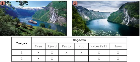
3.1 Semantic scene annotation . . . 35

3.2 Original multi-label data set . . . 39

3.3 Binary Relevance . . . 40

3.4 Label Powerset . . . 41

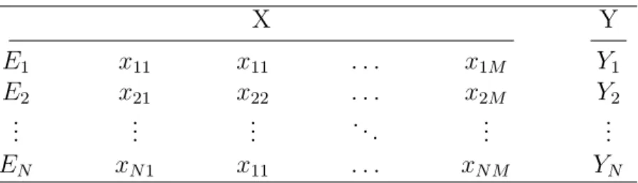
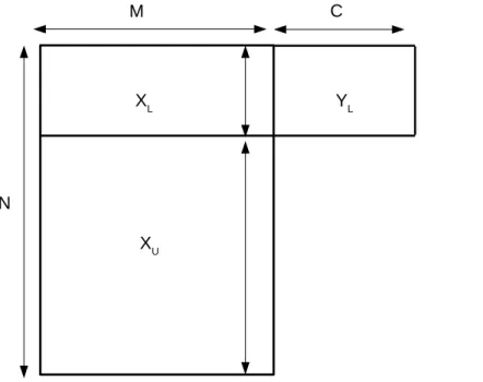
4.1 Data structure for semi-supervised multi-label learning. . . 61

4.2 General framework of S-CLS. . . 68

4.2 AUC v.s. number of selected features . . . 77

4.3 Nemenyi test diagram . . . 78

List of Tables

3.1 Multi-label data set . . . 36 4.1 Description of the data sets used in the experiments . . . 70 4.2 AUC and average rank . . . 77 4.3 Results (mean±std.) on all data sets used, over all measures (“&

indicates the smaller the better”; “_{% indicates the larger the better”). 79} 4.4 E↵ects of S-CLS on di↵erent classifiers. Before and after selection. . 81 4.5 Execution Time in Seconds . . . 82 5.1 Results (mean_{±std.) on all data sets used, over all measures (“&}

1 SC4 . . . 19 2 sSelect . . . 21 3 LSDF . . . 22 4 CLS . . . 23 5 CSFS . . . 26 6 SSDR . . . 30 7 BR-CLS . . . 62 8 LP-CLS . . . 63 9 S-CLS . . . 67 10 3-3FS . . . 89

“There is nothing more difficult to take in hand, more perilous to con-duct, or more uncertain in its success, than to take the lead in the in-troduction of a new order of things.”

Niccolo Machiavelli

1

Introduction

1.1 Context and Motivations

N

owadays, the rapid surge of high-throughput digital data acquisition tech-nologies has led to an exponential growth in the volume of the harvested data. Aided in this by an ever-increasing capabilities both in storage and computation. More than ever, a massive volume of data from various sources: digital cameras, sensors, patient records, stock market and retail transactions, gene sequencing, etc... is being collected at industrial scale oweing to ubiquitous and pervasive computing. Nevertheless, this deluge of data is not readily useful and needs to be processed and analyzed to extract meaningful knowledge. As John Naisbitt put it, “We are drowning in information and starving for knowledge” [Naisbitt84]. Unfor-tunately, the processing of such data is beyond human capacities, which calls for the need for e↵ective and efficient automation of the task. In this respect, machine learning o↵ers a plethora of data analysis tools and learning models. But sadly enough, virtually all learning models are challenged by the curse of dimensionality, which occurs when sample to feature ratio is too small [Duda12]. In fact, when

data is high-dimensional, many of the features describing them can be irrelevant and/or redundant. Which may have adverse e↵ect on learning models, and often leads to overfitting, downgrading performance and reduced intelligibility of the learning models [Fukunaga13].

In this regard, dimensionality reduction (DM) has proven to be the ultimate solution used to mitigate the nasty impacts of the curse of dimensionality. Funda-mentally, DM is based on the assumption that the intrinsic dimenionality of data often lies in a lower-dimension. This assumption paved the way to the development of a wide pectrum of algorithms and tools, but they basically all fall into two cate-gories: feature extraction and feature selection. In the former, the data is projected into a new space with a lower dimensionality made up of artefact features which are chiefly obtained by a linear mapping of the original features. Herein, the liter-ature abounds with well-known algorithms and widely used tools, among others, PCA [Jolli↵e86], LDA [Fisher36] and SVD [Alter00]. The main drawback of this approach is that it reduces the interpretability of the model learnt, as the original features are transformed and artificial features are created in the low-dimensional data. In contrast, feature selection techniques, uses statistical characteristics of the data to select from the original features the most representative and informa-tive features and discard the non relevant ones, thereby confers to feature selection a neat superiority over feature extraction, especially in terms of time complexity and better interpretability; quintessential examples of well-known feature selection techniques may include: Information Gain [Peng05], RelieFf [Robnik-ˇSikonja03], Fischer Score [Gu11].

More in particular, feature selection, also known as variable selection, consists in selecting from a feature space F , most discriminative features that would de-scribe instances in a given data set at least as well as the whole feature space does; that is without any deterioration in performance or lost information. In other words, as defined in [Garc´ıa15], feature selection is a process that chooses an opti-mal subset of features according to a certain criterion. In so doing, we do not only reduce time complexity, but also enhance accuracy and interpretability of learning algorithms (in classification or clustering tasks). Feature selection is commonly used on data sets with a huge amount of features (a.k.a variables) such as those used in: text processing [Schapire00], gene expression array analysis [Diplaris05], and combinatorial chemistry [Guyon03].

Section 1.1. Context and Motivations 3 Generally, feature selection is considered as a search problem aiming at ren-dering the optimal subset of features, in which we have 2M _{di↵erent subsets of}

features to consider, where M = |F | is the cardinality of the feature space. To this end, three parameters need to be specified before starting the search: the search direction, the search strategy, and the selection criteria. In fact, di↵erent search directions could be adopted to get the optimal subset: We can either be-gin from the whole feature space, and subsequently remove irrelevant features, or inversely start from an empty subset and add pertinent feature in each iteration, or start from both sides. This gives rise to three search directions: Sequential Forward Generation (SFG), Sequential Backward Generation (SBG), and Bidirec-tional Generation (BG). Another alternative that could be considered is to choose a random direction [Garc´ıa15].

In addition, di↵erent search strategies could be used: exhaustive search, con-sisting in exploring all possible subsets to find the optimal one; heuristic search that uses heuristics to conduct the search, preventing a brute force search but will certainly provide a non-optimal subsets, and non-deterministic search which is a combination of the previous two. The choice of a particular strategy is determined by finding a trade-o↵ between the optimality of the resulting subset and available resources (in terms of time and space). Finally, the selection criteria also have a great impact on the selection, since they are the real tools to measure the quality of the selected subset, the chosen criteria could emphasize performance either in terms of efficacy or efficiency. For instance in classification we could tend to favor the accuracy over other performance.

Furthermore, selection criteria are often used to produce a ranking in the fea-ture space. This ranking is basically achieved according to the type of the mea-sure in use, this can be: information meamea-sures, like the Information Gain (IG); distance measures, like Variance (generally applicable to numeric features); de-pendence measures, also known as measure of correlation. Other measures can be adopted, like consistency measures which is generally used to detect redundancies in selected subset of features or accuracy measures which relies on the performance of a particular classifier to select a particular set of features. However, these two last measures do not allow to produce a ranking.

From another perspective, feature selection can be categorized in many re-spects: the cardinality of the evaluated subset; the interaction with the

classifica-tion algorithm, if any; the availability and the amount of supervision informaclassifica-tion. From each of these aspects stems a di↵erent feature selection paradigm.

More precisely, feature selection algorithms evaluate the informational worth of features in two distinct ways: individual evaluation or subset evaluation (uni-variate/multivariate evaluation). On the one hand, the individual evaluation es-timates the worthiness of features independently of each others and assigns them weights (ranks) proportionate to their discriminative power (correlation with the class label). Numerous feature importance measures can be used in this regard. Obviously, this approach incurs less computational expenses. Nevertheless, the individual evaluation falls short of discovering redundant features as they are eval-uated in isolation from each others, so it might happen to have features with similar rankings. On the other hand, the subset evaluation approach can cope with both, feature relevance and feature redundancy. In contrast to individual evaluation, the subset evaluation is defined against a subset of features instead of individual features, however it induces higher computational cost.

Besides, considering the interaction or the lack thereof with the learning algo-rithm, feature selection can be achieved in various ways. Basically, the techniques developed so far come into three categories, namely: filter, wrapper and embedded selection [Guyon03]. The interaction with the learning algorithms is what makes the di↵erence among them. First, in the filter methods, there is no need to the learning algorithm to trigger the selection process. This is basically done by ex-ploiting the general characteristics of the data itself using certain statistics criteria. In the output every single feature will be associated with a score that determines its relevance. Second, the selection in wrapper methods is done by searching the space of the original features using a search strategy to get a subset that best fits the learning task in terms of certain evaluation measures. Finally, embedded methods incorporate the selection into the training stage of the learning process. Moreover, feature selection can be further organized in three more paradigms, ac-cording to the prior domain knowledge which could possibly guide the process of selection. In the supervised paradigm, the most discriminant features are those that are highly correlated with the class labels [Dash97]. Unsupervised feature selection is considered as a much more difficult problem. Roughly speaking, this task can be achieved by assessing the variance or the separability power of features [Dy04]. In the semi-supervised context, the task becomes more challenging with

Section 1.1. Context and Motivations 5 the so-called small-labeled-sample problem, in which the amount of data that is unlabeled can be much larger than the amount of labeled data [Zhao07]. Although feature selection is capable of dealing with all types of learning paradigm, the most well-known and frequently used field is classification.

In addition, most of the feature selection techniques developed in the last few years were mainly designed to support single-label learning. Wherein, each data instance is associated with only one class label, and the labels are mutually exclu-sive. This point of view is very restrictive, simplistic, and does not accommodate a lot of real-world application requirements. Motivated by this fact, the multi-label learning were introduced to allow instances to be associated with more than one class label simultaneously [Tsoumakas07a]. In fact, Multi-label learning is an emerging research field with an increasing number of applications, such as text categorizaiton [Schapire00], bioinformatics [Zhang06], and semantic scene annota-tion [Boutell04]. In this particular setting, the convenannota-tional single-label learning can be viewed as a particular case of multi-label learning. Unquestionably, this generality poses further challenges to feature selection which need to be addressed appropiately so as to take into account and take adavantage of the multi-label information[Zhang07b].

Standard solutions to multi-label classification follow two main strategies: problem transformation and algorithm adaptation. Problem transformation meth-ods suggest to convert the multi-label problem into one or more single-label problem upon which traditional single-label classification could be applied. On the other hand, algorithm adaptation approaches consist in extending traditional single-label algorithms in order to fit the “multi-labledness” of the data. To address dimensionality reduction in multi-label framework, feature selection follows suit of multi-label classification, thus the proposed solutions are either transformation-based or algorithm adaptation.

Multi-label feature selection is relatively a new research field and needs more attention from machine learning researchers and practitioners. Actually, in the cur-rent literature, little work were interested in multi-label dimensionality reduction and existing research studies are in their vast majority based on feature extrac-tion, and hardly ever focus on feature selection. In addiextrac-tion, the predominant approaches to multi-label feature selection are developed on the basis of problem transformation approach and rarely addressed multi-label selection directly. This

fact is even worse when dealing with semi-supervision and “multi-labeldness” con-jointly. In this context, we suggest various solutions to achieve feature selection from partially-labeled data.

1.2 Contributions

The research study conducted in this thesis is in the junction of various learn-ing paradigm. Chiefly, we put together semi-supervised, multi-label learnlearn-ing and feature selection. The ultimate goal is to develop new algorithms to address multi-label dimensionality reduction for small-multi-labeled-samples problems. In this particu-lar scheme, the thesis makes the following primary contributions:

• A general survey of graph theoretic-based semi-supervised feature selection, besides an overview of the available literature on multi-label classification and dimensionality reduction.

• The development and empirical evaluation of three filter feature selection algorithms for semi-supervised multi-label data sets. Using both prior infor-mation from the labeled part and the geometric structure of the unlabeled part of the data.

• An artifact solution to capture label importance by using a weighting mech-anism. At the output, each label is endowed with a weight encoding its im-portance in relation to the target concept underlying the data. Eventually, those label weighs will be integrated into the feature selection procedure. • An ensemble framework to solve semi-supervised multi-label feature selection

in the aim of alleviating the e↵ect of variance in the base algorithms.

More in particular, we introduce and empirically evaluate new feature selection algorithms we dubbed respectively: BR-CLS, LP-CLS, S-CLS [Alalga16] and 3-3FS. Each of which filters out relevant features through a specific objective function that is based on the Laplacian score. This objective function assigns a score to a feature according to its relevance to the target learning concepts, which in turn reflects its correlation to class labels and the ability to preserve the local structure of the data at the same time.

Section 1.3. Organization of the Thesis 7

1.3 Organization of the Thesis

Throughout this research study we give emphasis to feature selection from vari-ous perspectives. We shall touch on dimensionality reduction for semi-supervised data. The first two chapters are dedicated to a literature survey on single-label semi-supervised feature selection; and multi-label classification and dimensionality reduction. Afterwards the subsequent chapters detail our contributions to multi-label dimensionality reduction for the semi-supervised learning paradigm. For so doing, the remainder of this thesis is structured as follows:

• First in chapter 1.3, we provide an overview on semi-supervised feature se-lection. More specifically, the chapter gives insights into theoretical facets underlying the most prominent works on semi-supervised feature selection in single-label settings. We focus on methods developed in the light of spectral graph theory, which lay the groundwork for the development of our own algo-rithms. Before we go into the details of each of the methods, we first briefly introduce principles of spectral graph analysis and underline their relation with semi-supervised learning.

• Then, chapter 2.4 highlights theoretical and practical aspects of multi-label learning. To this end, this chapter is structured into two parts. First, we commence by defining and characterizing multi-label classification, present-ing some application domains and reviewpresent-ing strategies to perform multi-label classification. In the second part of the chapter, we address principles of dimensionality reduction for labeled data and review works on multi-label dimensionality reduction. Finally, the chapter concludes by presenting well-known tools recently coined to support and develop multi-label learning algorithms.

• In chapter 3.5, we present our framework to perform semi-supervised multi-label feature selection and discuss the foundational details of the proposed algorithms. We devise three filter feature selection algorithms based on spec-tral graph theory and a previous work on single-label feature selection (CLS [Benabdeslem11b]). The first two methods achieve multi-label dimension-ality reduction by applying CLS in conjunction with problem transforma-tion approaches. Subsequently a detailed descriptransforma-tion of our proposed S-CLS

(Soft-Constrained Laplacian Score) is presented. S-CLS achieves feature se-lection by exploiting prior domain knowledge expressed in terms of class labels from which we derive what we have called “soft-constraints” that will be integrated into the final feature importance measure. The experimental results are given solely for S-CLS which is the main contribution of this re-search. We shall compare our proposed algorithm with other state-of-the-art methods using various evaluation metrics and we shall prove the superiority of our algorithm by using statistical significance tests. Also, for the sake of fair comparison we shall use several benchmark data sets from various application domains.

• Subsequently chapter 4.5 presents an ensemble learning framework to S-CLS. We design an ensemble algorithm based on three-fold resampling. To be specific, we combine three subsampling techniques, each of which is applied on a di↵erent level of data. In 3-3FS, a Bagging is applied on the instance level, the Random Subsampling Method is conducted on the dimension level and finally a subsampling without replacement is performed on the label space level. The goal is to mitigate the e↵ect of variance on S-CLS and take more advantage of label correlation when performing dimensionality reduction. Some ensemble methods are then depicted and compared with; empirical results demonstrate that the proposed framework does improve the performance and the stability of S-CLS within reasonable computing costs. • Finally, chapter 5.6 winds up this thesis by a conclusion and presentation of

”Change your opinions, keep to your principles; change your leaves, keep intact your roots.”

Victor Hugo, Intellectual Autobiography

2

Semi-supervised Feature Selection

BThis chapter is devoted to feature selection in the context of semi-supervised learn-ing. Issues related to semi-supervised dimensionality reduction are discussed. In fact, like other learning paradigms, high dimensionality is also problematic to semi-supervised algo-rithms. Which grapple with the curse of dimensionality, tending to produce more complex and less e↵ective models. In this regard, we investigate how to bring the power of the spectral graph theory to design and implement convenient solutions to semi-supervised di-mentionality reduction. Throughout the chapter, we outline several algorithmic proposals developed in the light of spectral graph theory. C

Chapter outline

2.1 Introduction . . . 11

2.2 Generalities . . . 12 2.2.1 Notations . . . 12 2.2.2 Pairwise constraints . . . 13 2.2.3 Spectral Graph Theory . . . 15

2.3 Graph-theoretic Dimensionality Reduction . . . 18 2.3.1 Constraint Score For Semi-supervised Feature selection (C4) 18 2.3.2 Semi-supervised Feature Selection via Spectral Analysis

(sSelect) . . . 19 2.3.3 Locality sensitive semi-supervised feature selection (LSDF) 21 2.3.4 Constrained Laplacian Score (CLS) . . . 22 2.3.5 Constrained Selection-based Feature Selection (CSFS) . . 24 2.3.6 Semi-supervised Feature Selection for Regression

Prob-lems (SSLS) . . . 27 2.3.7 Semi-supervised Dimensionality Reduction (SSDR) . . . 28

Section 2.1. Introduction 11

2.1 Introduction

O

btaining fully labeled data is usually expensive, tedious and time-consuming, for more often than not it requires the endeavor of human experts. This gives rise to the so-called small-labeled sample problems, in which a large volume of un-labeled data is provided together with a tiny proportion of un-labeled ones [Zhu05]. This view seems to be more in line with most real-world applications, where it is prohibitively expensive to produce complete supervision over data. For example, in bioinformatics, protein sequences are churned out at industrial speed, but re-solving the functions of a single protein may require years of research e↵orts. In this regard, the limited amount of labeled data can be augmented by unlabeled data and eventually be utilized together to improve the learning performance. Nevertheless, it might happen that semi-supervised learning will not yield an im-provement. It might even be the case where using the unlabeled data leads to performance deterioration by misguiding the prediction. In reality, the feasibility of semi-supervised learning is conditioned by certain assumptions, which need to be satisfied [Chapelle09].

Inspirited by the success of semi-supervised learning, researchers have intro-duced semi-supervised learning to the field of dimensionality reduction. Likewise, semi-supervised dimensionality reduction is halfway between supervised and unsu-pervised dimensionality reduction, the goal is to use small amount of labeled data as additional information to improve the performance of unsupervised dimension-ality reduction. To confront high-dimensiondimension-ality in semi-supervised data, solu-tions come in various flavors reflecting di↵erent learning assumpsolu-tions. More pre-cisely, three basic assumption come into play when dealing with semi-supervision: the smoothness assumption, the manifold assumption and the cluster assumption [Chapelle09]; The smoothness assumption states that if two points x1, x2 are close,

then so should be the corresponding outputs y1, y2; the cluster assumption

conjec-ture that if two points are in the same cluster, they are likely to be annotated by the same class label; more importantly the manifold assumption assumes that the intrinsic structure of the data lies on a low-dimensional manifold embedded in the high-dimensional data space.

There exist some influential guidelines when dealing with semi-supervised data. In particular, it is usually the case to have various forms of partial supervision apart

from label information, e.g. pairwise constraints or a distance metric, which give some insights to guide the learning process in the absence of full prior domain knowledge. Another influential direction in the field of semi-supervised dimen-sionality reduction is the use of the graph theory analysis, whereby the data is represented by a graph encoding the underlying target concept. Basically, the graph is constructed according to a certain leaning assumption. In this perspec-tive, the dimensionality reduction is achieved by choosing the features that best preserve the inherent structure of the graph built. This global framework is gen-erally referred to as graph-theoretic dimensionality reduction. In this chapter, we overview diverse strands of the application of this general framework. But before-hand, it is important to review some theoretical concepts related to the field of semi-supervised dimensionality.

2.2 Generalities

This section lays the foundation to dimensionality reduction based on spectral graph theory. First, we give a formal description of semi-supervised feature se-lection and introduce some mathematical notations that will be used throughout the thesis. Secondly, we see an example of partial supervision exemplified by the concept of pairwise constraints, for which we give a formal definition and review some theoretical characteristics. Afterwards, we delve into the detail of the La-pacian graph theory. Finally, we investigate the foremost representative methods from the general graph-theoretic framework.

2.2.1 Notations

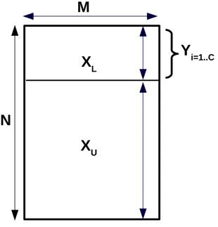
In semi-supervised learning, a data set of N instances X =_{x1, ..., xN} is divided

in two parts according to label availability: a supervised part XL={x1, ..., xL} in

which instances are associated with class labels from the set YL={y1, ..., yL}, and

an unsupervised part XU ={xL+1, ..., xL+U} comprising solely unlabeled instances.

In the small-labeled sample context, the total number of instances N = L + U , where L << U . Note that, two particular cases occur when L = 0 or U = 0, which bring us back to unsupervised/supervised learning, respectively.

Section 2.2. Generalities 13 In this setting, each data instance xi is a vector with M dimensions (features),

and labeled by the integer yi 2 {+1, 1}, if it belongs to XL. Let F1, F2, ..., FM

denote the M features of X and f1, f2, ..., fM be the corresponding feature vectors

that record the feature values in each instance. Figure 2.1 gives an example of semi-supervised data set.

Y

_i=1..C

X

_L

X

_U

M

N

Figure 2.1: A semi-supervised data set

Semi-supervised feature selection exploits XL together with XU to single out

the subset of most relevant features Fj1, Fj2, ..., Fjh of the target concept, where

h_{ M and j}r 2 {1, 2, ..., M} for r 2 {1, 2, ..., h}. Relevant features here, are those

that correlate with the class labels from XL, while at the same time preserve the

intrinsic geometric structure of the data in XU.

2.2.2 Pairwise constraints

Domain knowledge can be expressed in diverse forms, such as class labels, pair-wise constraints or any other kind of prior information. Undoubtedly, pairpair-wise constraints are the most practical; they are much cheaper to obtain, and do not require a deep knowledge about the data. As opposed to label information which need detailed information about the classes and instance affiliations. In other words, pairwise constraints provide weak and general supervision information, i.e.

they merely indicate for some pairs of instances whether they are similar and must be grouped together (must-link constraints), or dissimilar and cannot be put together (cannot-link constraints).

Pairwise constraints were first introduced in the field of semi-supervised cluster-ing [Wagsta↵01], where they are used to constrain the cluster buildcluster-ing by specifycluster-ing that instances in the must-link relation should be associated with the same clus-ter, and those in cannot-link relation should be assigned to di↵erent clusters. The incorporation of instance-level constraints has shown promising results and has even permitted to outperform conventional method clustering relying solely on the inner structure of the data. In the context of dimensionality reduction these two sets of constraints act as a guide in the attempt of digging out informative features which are those that satisfy the specified must-link and cannot-link constraints.

Constraints preservation, as a relevance criterion, could be used in supervised or semi-supervised frameworks, and has lead to the development of plethora of feature selection algorithms [Tang07, Zhang07a, Zhang08a]. In the presence of pairwise constraints, semi-supervised dimensionality reduction algorithms seek features that best help preserve the structure of data, while, at the same time, reduce the constraint violation.

Typically, the pairwise constraints are expressed in terms of two sets:

• Must-link, denoted by ⌦M L ={(xi, xj), such that xi and xj must be linked}

• Cannot-link, denoted by ⌦CL ={(xi, xj), such that xiand xjcannot be linked}

These instance-level constraints have several interesting properties which are generally used to extend their content. More specifically, Must-link constraints are equivalence relations, that is, symmetrical, reflexive and transitive. The tran-sitivity property allows to infer additional must-link relationships from the initial set [Bilenko04]. Cannot-link constraints, however, do not have such equivalence; (xi, xj) 2 ⌦CL^ (xj, xk) 2 ⌦CL does not necessarily implies that (xi, xk)2 ⌦CL.,

yet we can infer additional cannot-link constraints with the appropriate must-link and cannot-link constraints.

Formally:

• Transitive inference of Must-link constraints: (xi, xj) 2 ⌦M L ^ (xj, xk) 2

Section 2.2. Generalities 15 • Transitive inference of cannot-link constraints:(xi, xj) 2 ⌦CL ^ (xj, xk) 2

⌦CL =) (xi, xk)2 ⌦CL.

Commonly, a small-sized pairwise constraint subset is manually specified by a domain expert; the cardinality of a constraint subset is generally much lower than the total number of all possible combinations. On the other hand, it is also possible to derive such subsets automatically from the class label information, by stating that pairs of instances associated with the same class will be tied by a must-link constraint, and those pairs with di↵erent classes should be assigned to the cannot-link set. However, this cannot apply to multi-label learning, in chapter 3.5 we shall show how to generate appropriate constraints from multi-labeled data. Finally, when leveraging level-instance constraints to serve feature selec-tion, it would be wise to pay attention to incoherent/inconsistent constraints [Benabdeslem11a], for experiments had shown that they can have adverse e↵ects and harm the performance of feature selection algorithm. Also, all constraints are not equally important, so it would be appropriate to incorporate a constraint weighting algorithm in order to give more importance to critical constraints.

2.2.3 Spectral Graph Theory

To any graph we may associate a matrix which records information about its structure. The goal of spectral graph theory is to study the relationship between eigenvalues and eigenvectors of such matrices and how they relate the structure of the corresponding graphs [Chung97]. Spectral graph theory have found appli-cations in many fields, for instance one of Google’s first algorithms was based on spectral analysis by using eigenvectors to rank pages from the Internet [Page99]. Generally, machine learning tries to represent data by graphs on which spectral analysis techniques can be applied to gain useful insights into the data.

Indeed, the target concept underlying the data can be reflected by the structure of a graph. To be specific, a data set X is commonly modeled as a weighted graph G(V, E, w) characterized by its vertex set V , edge set E ✓ V V , and a weight function E _{! R}+_{. The vertices of the graph represent the instances, and the}

weighted edges encode the pairwise relationships. More specifically, the ith _vertex

vi ofG corresponds to xi 2 X. and there is an edge between each vertex pair (vi, vj)

relations than others, and a missing edge corresponds to a non-relation. Typically, the edges E and weights w in the data graph G denote similarities between nodes in V . The weight function is often used to represent pairwise instance similarities. These are often symmetric, resulting in an undirected graph.

When building the graph G we can consider several options:

• The ✏ neighborhood graph : Here we connect all points whose pairwise similarities are greater than ✏

• k nearest neighbor graph: we connect two nodes vi and vj if the

cor-responding instances xi and xj are among the k-nearest neighbors of each

other.

• The fully connected graph: Here we simply connect all points with positive similarity with each other, and we weight all edges by wij.

Typically, the graph G is built by using the nearest neighbors of each point; this ensures that the graph is sparse, which will speed up computation.

Besides, the similarities can be expressed in various ways : geometric struc-ture, class label information or pairwise constraints, this has given rise to various learning algorithms. For instance, using class information, the similarity function could be defined by:

wi,j = 8 < : 1 nl yi = yj = l 0 otherwise (2.1)

In the absence of prior knowledge, a similarity function could be based on the geometric structure of the data, e.g. a kernel function based on Euclidean distance between data points; the most used function is the Gaussian kernel defined by:

wij = e

kxi xjk2

(2.2) Given the similarity function, we define the positive semi-definite adjacency matrix as follows:

Section 2.2. Generalities 17 Aij = 8 < : wi,j if (i, j)2 E 0 otherwise (2.3)

In the context of feature selection, the adjacency matrix is commonly referred to as the similarity matrix and denoted by S

From the adjacency matrix we can compute the degree matrix D of the graph G, which is defined by D = diag(S1), 1 = [1, . . . , 1]T_.

The degree matrix can be interpreted as an estimation of the density around xi since the more points that are close to xi the larger Dii

Given the adjacency matrix A and the degree matrix D of G, the Laplacian matrix for the weighted undirected graph G, also known as graph Laplacian is defined by:

L = A D (2.4)

The graph Laplacian satisfies the following properties: L is symmetric, positive semi-definite and xT_{Lx =}P

i,j(xi xj)2

In practice, it is common to normalize the graph Laplacian to account for the fact that some nodes are more highly connected than others, the normalized Laplacian matrix is defined by:

L = D 12LD 1

2 (2.5)

In view of the graph theory, the learning process can be reduced to performing eigen-decomposition problems. More in particular, the clustering problem can be formulated as follows: We want to partition the graph such that the edges between di↵erent groups have low weights and the edges within a group have high weights. In feature selection we seek features that are consistent with the graph structure; features that assign similar values to instances that are near each other (strongly connected in the graph). The next section reviews state-of-the-art methods developed in the highlights of the principle of graph theory.

2.3 Graph-theoretic Dimensionality Reduction

This section exposes methods that rely on spectral analysis to achieve semi-supervised dimensionality reduction. In fact, relevant features are consistent with the target concept (in supervised learning the target concept is related to class affiliation and in unsupervised learning the target concept is encoded in the innate structure of the data) which, as we have seen above, can be captured by the struc-ture of a graph. Therefore, analyzing the strucstruc-ture of similarity graphs to spot relevant features has resulted in a plethora of dimensionality reduction methods, each of which is characterized by its specific definition and building of the under-lying similarity graphs. The common denominator of all these methods, referred to as graph-theoretic methods, is the graph based-assumption.

The graph-based assumption states that if d(xi, xj) is small, then yi ⇡ yj, In

plain words, this means that the similarity between two points is proportional to their distance. This assumption applies regardless of the availability of the class information. Below, we go into the details of some algorithms that fall in the graph-theoretic framework.

2.3.1 Constraint Score For Semi-supervised Feature selection

(C4)

Feature selection in mixed data sets can be achieved by hybridizing supervised and unsupervised algorithms. The hybridization can be as trivial as a mere product between score functions. In this line of thinking, [Kalakech11] proposed a semi-supervised constraint score by combining the Laplacian Score (LS) [He05a] and the Constraint Score (CS) [Zhang08b], two popular spectral graph based feature selection algorithms. Wherein, the Laplacian score is applied to the unlabeled part of the data and the Constraint Score seeks relevant features in the labeled part. The objective score function for a feature fr, which needs to be minimized,

is defined as:

Section 2.3. Graph-theoretic Dimensionality Reduction 19 where LSr and CSr are the Laplacian Score and the Constraint Score for the fr

computed from the labeled and the unlabeled parts of the data, respectively. For the mathematical detail about both scores, see [He05a] and [Zhang08b].

A worthwhile mentioning study in this work in which the authors considered the fact that constraint-based algorithms are highly sensitive to changes in the con-straint sets. In terms of feature selection, this means that changing the concon-straints subsets might lead to change in feature ranks, which eventually lead to di↵erent subsets of selected features. To resolve this issue, some work has suggested to use multiple constraint sets within the framework of ensemble learning [Sun10].

The phenomenon has been thoroughly discussed by Kalakch et al., where the authors suggested to use the Kendall’s Coefficient [Grzegorzewski06] to measure how the feature ranks vary with respect to di↵erent subsets of constraints. The Kendall’s Coefficient, which value lies in [0, 1], examine the concordance between feature ranks for di↵erent feature selection algorithms; the lower the Coefficient the less sensitive is the algorithm. The authors have empirically demonstrated that their Cr4 is less sensitive to constraint changes than other methods they compared

with.

Algorithm 1 SC4

Input: Data set X, pairwise constraints sets ⌦M L, ⌦CL and (a tuning

param-eter in the Laplacian Score, with default value =100) Output: The ranked features

for r = 1 to M do

1: Calculate LSr, the Laplacian score of Fr.

2: Calculate CSr, the Constraint score of Fr.

3: Calculate SC4r, the score of Fr using eq.(2.6)

end for

4: Rank the features according to their scores in ascending order.

2.3.2 Semi-supervised Feature Selection via Spectral Analysis

(sSelect)

Based on the clustering assumption, Authors in [Zhao07] resorted to clustering techniques to solve the semi-supervised feature selection. In this spirit, the large amount unlabeled data is used to shape the cluster structure, whereas the role of

the labeled data is to guide the clustering operation. The spectral analysis is used to find the optimal solution to the so-defined clustering problem.

Basically, the proposed approach uses the feature vectors to construct cluster indicators for the clustering algorithm, here the normalized min-cut. the fitness of cluster indicators will determine the relevance of the corresponding features. The passage from a feature vectors to a cluster indicator is assured by a function called the F-C Transformation, defined as:

g_r= ✓(fr) = fr

fT r D1

1TD1.1; (2.7)

Where fr 2 Rn and 1 = (1, . . . , 1)T.

The fitness of cluster indicator is determined by two factors: separability and consistency. The separability indicates how well separable are the cluster structure, which reflects the unsupervised point of view. On the other hand, the consistency shows the degree of agreement between the cluster structure and label information, reflecting the supervised point of view. In the ideal case, all labeled data of each cluster should come from the same class.

To find the best clustering, the normalized min-cut seeks to find a cut for G induced from the data X according to spectral graph theory, which minimizes the cost function defined by:

⌘g T rLgr gT rDgr (2.8) Where ⌘ is a regularization parameter. Mathematically speaking, the fitness of a cluster indicator is evaluated by the following regularization framework:

sSelectr = ⌘ gT rLgr gT rDgr + (1 ⌘)(1 N M I(ˆg, YL)) (2.9)

Where N M I is the normalized mutual information. ˆg = sign(g)2 _{and is used}

to map the cluster indicators to classes.

The score sSelectr for a feature frreflects its relevance: the smaller the value of

the score, the more relevant the feature. In the equation, the first term calculates the cut value of g (best clustering indicators are associated with minimum values), while the second term uses the normalized mutual information to estimate the accuracy of the clustering-induced classification. The regularization parameter ⌘

Section 2.3. Graph-theoretic Dimensionality Reduction 21 is set empirically to favor either the impact of the unlabeled data or the labeled data in the fitness score.

Algorithm 2 sSelect Input: Data set X, ⌘, k

Output: the ranked features list

1: Construct the k-nearest neighbors graph G from X

2: Build the dissimilarity matrix S , the degree matrix D and the Laplacian matrix L from G

for r = 1 to M do

3: Construct the cluster indicators gr from Fr using eq.(2.8)

4: Calculate sSelectr, the score of the feature Fr using eq.(2.9)

end for

5: Rank the features according to their scores in descending order.

2.3.3 Locality sensitive semi-supervised feature selection (LSDF)

Authors in [Zhao08] introduced a new algorithm based on manifold learning and spectral graph analysis. In the context of the spectral theory, the proposed ap-proach builds two distinct graphs: a within-class graph Gw and a between-class

graph Gb, in order to express the local geometrical and discriminant structure of

the data. The importance of features is then calculated according to their power of preserving the structure of the two graphs.

The graph Gw connects instances with the same label or sufficiently close to

each other, while Gb connects instances with di↵erent labels. The similarity

ma-trices of these graphs are computed as follows:

Sw,ij = 8 > > > < > > > :

if xi and xj share the same label

1 if xi or xj is unlableled, but xi 2 KNN(xj) or xj 2 KNN(xi) 0 otherwise (2.10) Sb,ij = 8 < :

1 if xi and xj have di↵erent labels

Where KN N (xi)/KN N (xj) denotes the sets of k nearest neighbors of xi/xj

respectively, and is a suitable constant empirically set to 100. The graph Laplacians of Gw and Gb are defined by:

Lw = Dw Sw, Dw = diag(Sw1) Lb = Db Sb, Db = diag(Sb1)

Where Dw and Db are the degree matrices of Gw and Gb respectively.

The pertinence of a feature is then measured by the following objective function, which needs to be maximized:

Lr= fT r Lbfr fT r Lwfr (2.12) for r = 1, 2, . . . , M.

Features with the highest scores are ranked first and will be eventually selected. The score is self-explanatory, the most informative features are those for which the within-class and between-class graph structure are best preserved. Loosely speaking, a feature is considered relevant if at this dimension nearby points, or points sharing the same label, are close to each other, while points with di↵erent labels are far apart. Algorithms 3 outlines all steps of LSDF.

Algorithm 3 LSDF Input: Data set X, , k

Output: List of ranked features

1: Construct the within-class and the between-class graphs (Gw, Gb) from X

2: Compute the weight matrices Sw and Sb, the degree matrices Dw and Db, and

the Laplacian matrices Lw and Lb from Gw and Gb respectively

for r = 1 to M do

4: Calculate Lr, the score of the feature Fr using eq.(2.12)

end for

5: Rank the features according to their scores in descending order.

2.3.4 Constrained Laplacian Score (CLS)

Another attempt to bridge the chasm between unsupervised and supervised feature selection can be found in [Benabdeslem11b]. The authors devised a more elaborate aggregation of Laplacian score and Constraint score. The proposed score–CLS,

Section 2.3. Graph-theoretic Dimensionality Reduction 23 benefits from both the data structure and the supervision information to pinpoint discriminative features.

More concretely, CLS tends to select features with the best locality and con-straints preserving abilities. The justification for this is quite intuitive, on one hand, a relevant feature is expected to have close values for instances linked by a Must-link constraint and/or nearby instances, and disparate values for faraway instances or those in the Cannot-link subset.

To this end, CLS builds two distinct graphs: the dissimilarity graph Gkn

repre-senting data points in the Cannot-link set, and the neighborhood/ similarity graph GCLconnecting neighbor data points and/or those belonging to the Must-link set.

In this particular setting, the importance of a feature is the degree to which it respects the structure of these two graphs.

From the above the objective function of CLS is formulated as follows:

CLSr = P i,j(fri frj)2Sij P i P j|9k,(xk,xj)2⌦CL(fri ↵ i rj)2Dii (2.13) where : Sij = 8 > < > : e kxi xjk 2

if xi and xj are neighbors or (xi, xj)2 ⌦M L

0 otherwise (2.14) and: ↵i_rj = 8 < : frj if (xi, xj)2 ⌦CL µr otherwise (2.15)

Note that if there are no labels (L = 0 and X = XU) then CLSr = LSr and

when (U = 0 and X = XL), CLS represents an adjusted CSr, where the M L and

CL information would be weighted by Sij and Diirespectively in the formula.The

Algorithm 4 CLS

Input: Data set X(N M ), the constant , the neighborhood degree k 1: Construct the constraint sets (⌦M L and ⌦CL) from YL

2: Construct the graphs Gkn and GCL from (X, ⌦M L) and ⌦CL respectively.

3: Calculate the weight matrices Skn, SCL and their Laplacians Lkn, LCL re-spectively.

for r = 1 to M do

4: Calculate CLSr according to eq.(2.13).

end for

5: Rank the features Fr according to their scores CLSr in ascending order.

It would be important to note that the method also favors features with high representative power (high variance).

Experiments have shown that CLS gives good performance in comparison with other state-of-the-art methods, nonetheless exhibits high sensitiveness to noise in the constraint sets ( incoherence/inconsistency), which may lead to downgraded performance.

2.3.5 Constrained Selection-based Feature Selection (CSFS)

In the endeavors to leverage the pairwise constraints in feature selection, [Hindawi11] proposed an algorithm called CSFS which tries to alleviate sensi-tivenss with respect to constraints. CSFS is motivated by the empirical observa-tion that ”some” constraints may have adverse e↵ect on performance [Davidson06]. Indeed, incoherent/contradictory pairwise constraints are harmful. It is important to mention that the incoherence is not due to noise or error; the constraints could be directly derived from the label information, and yet be incoherent.

The coherence is a measure proposed to quantify the degree of agreement be-tween constraints. Constraints can be regarded as ”attractive/repulsive” forces in the feature space. In this sense, two constraints are incoherent if they exert con-tradictory forces ( have parallel force vectors) in the same vicinity, and coherent if their force vectors are orthogonal. With this in mind, it suffices to compute the projected overlap of each constraint vector on the other to determine their coherence. That is, two constraints are coherent if their corresponding projected overlap is equal to zero.

Section 2.3. Graph-theoretic Dimensionality Reduction 25 The above can be stated formally as follows: Let m 2 ⌦M L, c 2 ⌦CL be

two constraint vectors connecting two points, the coherence of a constraint set ⌦ = ⌦M L[ ⌦CL is given by: COH(⌦) = P m2⌦M L,c2⌦CL (overmc = 0^ overcm = 0) |⌦M L| |⌦CL| (2.16)

Where overmc represents the distance between the two projected points linked by

m over c. is the number of the overlapped projections.

With this quantification, one e↵ective way to lessen negative e↵ects of inco-herence is to perform constraint selection prior to the learning task. More in particular, before submitting the constraint set to the selection algorithm, it is beneficial to apply a kind of coherence-based constraint selection to filter out inco-herent constraints. To be selected a constraint needs to be fully coinco-herent with other constraints (zero projected overlap with all available constraints). The complete algorithm is outlined in Algorithm 5

The objective function of the score is formulated as follows:

'r = P i,j(fri frj) 2 (Sij + Nij) P i fri ↵irj 2 Dii (2.17) Where: Sij = 8 > < > : e kxi xjk 2

if xi and xj are neighbors

0 otherwise

(2.18)

Nij = 8 > > > > > > > > > > > > > > > < > > > > > > > > > > > > > > > : e kxi xjk 2

if xi and xj are neighbors and (xi, xj)2 ⌦0M L

e kxi xjk

2!2 if xi and xj are neighbors and (xi, xj)2 ⌦ 0 CL

OR

if xi and xj are not neighbors and (xi, xj)2 ⌦0M L

0 otherwise (2.19) And: ↵i_rj = ( frj if (xi, xj)2 ⌦0CL µr otherwise (2.20) Where ⌦0

CL and ⌦0M L denote the new constraint subsets (comprising only

co-herent constraints), is a constant to be tuned. xi, xj are neighbors in the sense

that xi is among the k-nearest neighbors of xj and vice-verse. µr = 1_nP_ifri is the

mean of the column corresponding to the feature fr.

Note that the term Nij is introduced to penalize bad cases corresponding to

distant instances related by Must-link constraints, and inversely nearby instances related by Cannot-link constraints.

Another major contribution of the method stems from the observation that a fixed number of neighbors k could be misleading when defining the local structure of the data. In fact, A score based on k-nearest neighbors graph could be biased by far neighbors, and thus fail to capture the real locality structure of the data. To fix this issue, the authors proposed to conduct a similarity-based clustering to determine the appropriate k. So that two instances are neighbors if they belong to the same cluster. In this particular setting, k is equal to the number of instances in each cluster and varies in each data set. To obtain an optimal partition, the authors chose to apply AHC(Ascendant hierarchical clustering) using Davies Bouldin as internal index.

Section 2.3. Graph-theoretic Dimensionality Reduction 27 Algorithm 5 CSFS

Input: Data set X(N M ), the constant Output: Ranked features

1: Construct the constraint set (⌦M L and ⌦CL) from YL

2: Select the coherent set (⌦0_{M L} and ⌦0_CL) from (⌦M L and ⌦CL) based on 2.16

3: Construct the graphs Gkn and GCL from (X, ⌦0M L) and ⌦0CL respectively.

4: Calculate the weight matrices Skn, Nkn and SCL and the Laplacians Lkn, LCL.

5: for r = 1 to M do

6: Calculate 'r according to eq.(2.17)

7: end for

8: Rank the features Fr according to their scores 'r in ascending order.

In the sequel of their research works, the same authors developed two other methods, named CSFSR [Benabdeslem14] and ECLS [Benabdeslem16], which are designed to tackle issues related to feature redundancy and ensemble learning, respectively.

Till now we have seen various scenarios where feature selection benefits classi-fication or clustering tasks. Next, we present a di↵erent example that shows that feature selection could also be useful in regression problems.

2.3.6 Semi-supervised Feature Selection for Regression Problems

(SSLS)

It is well established that redundant and uninformative features decrease perfor-mance and make learning algorithms prone to overfitting. This statement holds true for regression problems. In regression problems, the task is to learn a mapping from the space feature to the output space whose values are defined on R.

In this particular setting, [Doquire13a] devised a new feature selection criterion which is inspired by the Laplacian Score. The goal is to choose features according to their ability of preserving the locality structure of the data. With the particularity here that the prior information (class labels) is expressed in terms of continuous values.

To this end, the authors first developed a supervised version of the score upon which they built a semi-supervised variant. The underlying assumption is that

close instances have close output values, and therefore best features are expected to have close values for instances with close outputs.

According to that assumption, authors developed the similarity matrix Ssup

defined by: Ssup_ij = 8 < : e (yi yj ) 2

if xi and xj are close

0 otherwise

(2.21)

The supervised version of the score called SLS, which should be minimized, is then defined as follows:

SLSr = ˜ fT r Lsupf˜r ˜ fT r Dsupf˜r (2.22) where

Dsup _{= diag(S}sup_{1), L}sup _{= D}sup _Ssup_{, ˜f} r = fr

frTDsup1

1T_Dsup₁1

The explanation of the objective function is straightforward. The first term helps preserve the local geometrical structure of the data by keeping features that are most coherent with the above-defined similarity measure, while the second term is used to discard features associated with low variance since they do not have much descriptive power; the same as in the Laplacian Score.

In the semi-supervised variant of the SLS Score, the similarity measure have to be rethought to incorporate information from the unlabeled data. To this end, [Doquire13a] defined a new distance function that computes pairwise distances between instances from the whole data set.

dij =

8 < :

(yi yj)2 if yi and yj are unknown 1

n

Pn

k=1(fki fkj)2 otherwise

(2.23)

Once the pairwise distances are set, the SSL Score is reformulated into a semi-supervised one (SSLS) as follows:

SSLSr = ˜ fT rLsemif˜r ˜ fT r Dsemif˜r SLSr (2.24)

Section 2.3. Graph-theoretic Dimensionality Reduction 29 where the similarity matrix is redefined as:

Ssemi_ij = 8 > > > < > > > :

e di,j if xi and xj are close and yi and yj are unknown

Ce di,j if xi and xj are close and yi and yj are known

0 otherwise

(2.25)

Where, the positive constant C is supposed to give more importance to the supervised part of the data. The closeness here is to be understood in the sense of k-nearest neighbors.

The same justification mentioned above applies for the semi-supervised version of the score. The score permits to retain features with high locality structure preserving ability and high predictive power. Finally, it is worthwhile mentioning that both the equations 2.22 and 2.24 are thoughtfully designed to give more importance to the labeled part of data sets, the reason is that we naturally trust more the known than the unknown.

2.3.7 Semi-supervised Dimensionality Reduction (SSDR)

Feature extraction seeks informative and non-redundant features by finding a map-ping of a high-dimensional space into a space of fewer dimensions. The new space consists of features that are calculated as a function of the original features. In this context, [Zhang07a] proposed a feature extraction algorithm that uses both prior supervision information in the form of instance-level constraints along with the structure of the unlabeled data. The principle that underpins this approach is to compute from the original feature space a low-dimensional representation that will preserve the intrinsic structure of the data and satisfies the pairwise constraints at least as well as the original feature space does.

More concretely, find the projective vectors W and compute the artificial sub-stitute features yi = WTxi that accommodate the intrinsic structure of the data

and comply with the pairwise constraints. For the reason that instances sharing a must-link relation should be close and those in a cannot-link relation should be far away. This leads to the development of the following objective function, which needs to be maximized:

J(w) = 1 2n2 X (xi,xj)2C (wTxi wTxj)2 + ↵ 2nC X (xi,xj)2C (wTxi wTxj)2 2nM X (xi,xj)2M (wTxi wTxj)2 (2.26)

Where nC, nM is the number of instances in the Cannot-link and the

must-link sets respectively. ↵, are trade-o↵ parameters to balance the impact of the di↵erent terms. The formula is self-explanatory, the main goal is to keep distances between instances in the must-link set as small as possible and distances between instances in cannot-link set as large as possible. Similar to PCA [Jolli↵e86], the first term enforces the global covariance structure of the data.

From spectral graph point of view, the equation could be reformulated as fol-lows: J(w) = 1 2 X i,j (wTxi wTxj)2Si,j (2.27) where Sij = 8 > > > < > > > : 1 n2 + _nC↵ if (xi, xj)2 C 1 n2 _nM if (xi, xj)2 M 1 n2 otherwise (2.28)

By further algebraic developments we have J(w) = wT_XLXT_{w, where L is the}

Laplacian matrix. The last equation is a typical eigen-problem which can be solved by finding the eigenvectors of XLXT _{corresponding to the largest eigenvalues. The}