HAL Id: hal-02882394
https://hal.archives-ouvertes.fr/hal-02882394
Submitted on 26 Jun 2020HAL is a multi-disciplinary open access
archive for the deposit and dissemination of sci-entific research documents, whether they are pub-lished or not. The documents may come from teaching and research institutions in France or abroad, or from public or private research centers.
L’archive ouverte pluridisciplinaire HAL, est destinée au dépôt et à la diffusion de documents scientifiques de niveau recherche, publiés ou non, émanant des établissements d’enseignement et de recherche français ou étrangers, des laboratoires publics ou privés.
General formulation of macro-elements for the
simulation of multi-layered bonded structures
Sébastien Schwartz, Eric Paroissien, Frederic Lachaud
To cite this version:
Sébastien Schwartz, Eric Paroissien, Frederic Lachaud. General formulation of macro-elements for the simulation of multi-layered bonded structures. Journal of Adhesion, Taylor & Francis, 2020, 96 (6), pp.602-632. �10.1080/00218464.2019.1622420�. �hal-02882394�
an author's https://oatao.univ-toulouse.fr/23949
https://doi.org/10.1080/00218464.2019.1622420
Schwartz, Sébastien and Paroissien, Eric and Lachaud, Frédéric General formulation of macro-elements for the simulation of multi-layered bonded structures. (2020) Journal of Adhesion, 96 (6). 602-632. ISSN 0021-8464
1 General formulation of macro-elements for the simulation of multi-layered bonded structures.
Sébastien Schwartz1,2,*, Eric Paroissien2 , Frédéric Lachaud2 1
SOGETI High Tech, R&D Dpt., Aeropark, 3 Chemin de Laporte, 31100 Toulouse, France 2
Institut Clément Ader (ICA), Université de Toulouse, ISAE-SUPAERO, INSA, IMT MINES ALBI, UTIII,
CNRS, 3 Rue Caroline Aigle, 31400 Toulouse, France
*To whom correspondence should be addressed. E-mail: [email protected]
Abstract – Adhesively bonded joints are often addressed through Finite Element (FE). However, analyses based on FE models are computationally expensive, especially when the number of adherends increases. Simplified approaches are suitable for intensive parametric studies. Firstly, a resolution approach for a 1D-beam simplified model of bonded joint stress analysis under linear elastic material is presented. This approach, named the macro-element (ME) technique, is presented and solved through two different methodologies. Secondly, a new methodology for the formulation of ME stiffness matrices is presented. This methodology offers the ability to easily take into account for the modification of simplifying hypotheses while providing the shape of solutions, which reduced then the computational time. It is illustrated with the 1D-beam ME resolution and compared with the previous ones. Perfect agreement is shown. Thirdly, a 1D-beam multi-layered ME formulation involving various local equilibrium equations and constitutive equations is described. It is able to address the stress analysis of multi-layered structures. It is illustrated on a double lap joint (DLJ) with the presented method.
Key words: macro-element; multi-layered; ordinary differential equation procedure; analytical models; stress analysis; aeronautical.
2 NOMENCLATURE AND UNITS
Aj extensional stiffness (N) of adherend j
Bj extensional and bending coupling stiffness (N.mm) of the adherend j Dj bending stiffness (N.mm²) of the adherend j
Ea Young’s modulus (MPa) of the adhesive Ej Young’s modulus (MPa) of the adherend j Ga Coulomb’s modulus (MPa) of the adhesive Gj Coulomb’s modulus (MPa) of the adherend j kI,i peel stiffness (MPa/mm) of the adhesive i kII,i shear stiffness (MPa/mm) of the adhesive i
kv peel stiffness (MPa/mm) of the spring of the adhesive in the SLJ geometry ku shear stiffness (MPa/mm) of the spring of the adhesive in the SLJ geometry kvi peel stiffness (MPa/mm) of the spring of the adhesive i in the DLJ geometry kui shear stiffness (MPa/mm) of the spring of the adhesive i in the DLJ geometry K stiffness matrix
U vector of nodal displacements F vector of nodal forces
C vector of integration constants
Y vector of differential equations solution
S peel stress (MPa) of the adhesive
Si peel stress (MPa) of the adhesive i T shear stress (MPa) of the adhesive
Ti shear stress (MPa) of the adhesive i
Vj shear force (N) of the adherend j in the y direction Nj normal force (N) of the adherend j in the x direction
3
b width (mm) of the adherends
ej thickness (mm) of the adherend j tj thickness (mm) of the adhesive j
lj length (mm) of the out-bonded adherend j Lj length (mm) of the bonded adherend j
uj displacement (mm) of the adherend j in the x direction vj displacement (mm) of the adherend j in the y direction
θj angular displacement (rad) of the adherend j around the z direction P(x) characteristic polynomial
λi eigenvalues i Vi eigen vectors i P basis change matrix ⊕ direct sum
Ji Jordan block i 𝛿 Kronecker delta
det determinant of a matrix dim dimension of a matrix or vector ker kernel of a matrix
Re(x) real part of x Im(x) imaginary part of x
(x,y,z) system of axes FE Finite Element ME macro-mlement
ODE ordinary differential equation SLJ single lap joint
4 1. Introduction
In the frame of the design of lightweight structures such as aircraft structures, the proper choice of joining technology is decisive for its life. If the mechanical fastening, including riveting or screwing, is the joining technology the most used on aircraft structures, adhesive bonding may offer significantly improved mechanical performance in terms of stiffness, static strength and fatigue strength [1–4]. For example, according to Higgins, adhesive bonding has been and is used for joining stringers to fuselage and wing skins, in order to stiffen them against buckling [2]. The Finite Element (FE) method is able to address the stress analysis of bonded joints. Nevertheless, since analyses based on FE models are computationally costly, it would be profitable both to restrict them to refined analyses and to develop for designers simplified approaches, enabling extensive parametric studies. Numerous simplified stress analyses of bonded joints are available and provide accurate predictions [5–7]. In 1938, Volkersen published a shear lag model for the prediction of the adhesive shear stress distribution along the overlap [8]. It was the first stress analysis including the deformation of adherends. The adhesive layer was simulated as an elastic foundation of shear springs. In 1944, Goland and Reissner provided the first closed-form solution of distributions of adhesive shear stresses along the overlap for simply supported balanced joint made of adherends undergoing cylindrically bending [9]. The approach used by Goland and Reissner involved two steps: (i) analysis of the bonded overlap leading to integration constants and (ii) analysis of the parts outside the bonded overlap providing the required boundary conditions. This approach is related to the sandwich-type analysis concept for the stress analysis of bonded joints. Goland and Reissner took into account the geometrical non-linearity due to the lag of neutral line to assess the bending moment at both overlap ends, as boundary conditions for the adhesive stress distributions, through a bending moment factor. The sandwich-type analysis concept was then employed by other researchers to improve this initial model to take into different local equilibriums, different constitutive behaviors and various geometries [10–20] eventually leading to various forms of the bending moment factor. Nevertheless, as function of the set of initial simplifying hypotheses, it is not always possible to get closed-form solutions of adhesive
5 stress distribution. Twenty years ago, Mortensen et al. provided then a resolution scheme based on the numerical integration of first order ordinary differential equations (ODEs) allowing to take account various boundary conditions, geometries and material behaviors [21–23]. The authors of the present papers and co-workers have been working on the development of the macro-element (ME) technique for the simplified stress analysis of bonded, bolted and hybrid (bonded/bolted) joints [24–32]. Dedicated 4-nodes Bonded-bars (BBa) and Bonded-beams (BBe) have been formulated. As for the JE model, only one BBa or BBe, depending on the chosen kinematics, is sufficient to be representative for an entire bonded overlap in the frame of a linear elastic analysis (see Fig. 1). When the geometrical or material properties of the adherends or the adhesive layer vary along the overlap, a mesh is necessary along the overlap length direction only. The ME technique is inspired by the FE method and differs in the sense that the interpolation functions are not assumed. Indeed, they take the shape of solutions of the governing ordinary differential equations (ODEs) system, coming from the constitutive equations of the adhesive and adherends and from the local equilibrium equations, related to the simplifying hypotheses. The main work is thus the formulation of the elementary stiffness matrix of the ME. Once the stiffness matrix of the complete structure is assembled from the elementary matrices and the boundary conditions are applied, the minimization of the potential energy provides the solution, in terms of adhesive stress distributions along the overlap, internal forces and displacements in the adherends. The ME technique can be regarded as mathematical procedure allowing for the resolution of the system of ODE, under a less restricted application field of simplifying hypotheses, in terms of geometry, material behaviors, kinematics, boundary conditions and loadings. In the case of bar kinematics, the closed-form expressions for the stiffness matrix components were provided [24, 27, 28, 32] as well as the shape of adhesive shear stress, adherend displacements and forces. The minimization of the potential energy allows then for the assessment of integration constants. In the case of beam kinematics, if the closed-form expressions for the stiffness matrix components were not provided, those for the adhesive shear and peel stresses, adherend displacements and forces were established after a long work [24, 27, 28]. To speed up the formulation
6 of new MEs under various sets of hypotheses, another approach has been developed, based on the resolution of the first order ODEs using the exponential matrix. However, the closed-form expressions for adhesive stresses, adherend displacements and forces are not any more provided, so that a meshing along the longitudinal axis is required to assess them along the overlap. If the configuration to be simulated, such as functionally graded or mixed adhesive joints or joints involving non-linear materials, needs a mesh this drawback does not have any consequence in terms of computational time. Nevertheless, in the case homogeneous adhesive joints or joints involving linear material behaviors, the computational time is increased. The objective of this paper is to provide a methodology to formulate new MEs while providing the shape of solutions for the adhesive peel and shear stresses, adherend displacements and internal forces. Firstly, the new method is explained and applied to the original linear elastic 1D-beam model for the stress analysis of a SLJ joint. Secondly, a ME representing for the layering of n adherends is described. Thirdly, the particular case of double lap joint (DLJ) is presented.
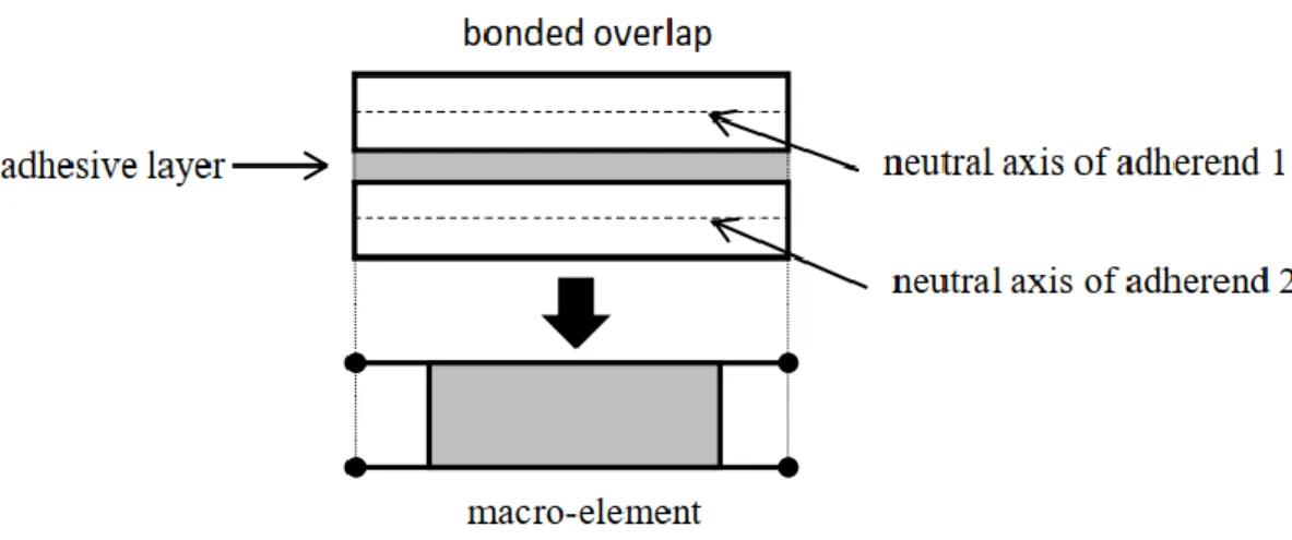
Figure 1. Equivalent modelling of a bonded overlap by a macro-element.
2. Linear Elastic 1D-Beam Model 2.1. Overview
The method presented in this article is applied on the formulation of a ME. A ME is a special finite element developed by Paroissien [24]. It provides the resolution of the bonded overlap system of
7 governing ODEs. The displacements and forces of both adherends, as well as the adhesive stresses, are then computed. The simplified linear elastic 1D-beam model is a bonded overlap element using four nodes. The outer adherends are Euler-Bernoulli laminated beam. According to the classical Finite Element method, the stiffness matrix of the entire structure K is assembled and the selected boundary conditions are applied. Then, solving the equation F=KU, where F is the vector of nodal forces and U is the vector of nodal displacements, leads to the minimization of the potential energy. Using the ME technique offers the possibility to simulate complex structures, such as single-lap bonded joints at low computational costs. The model is based on the following hypotheses:
- the adherends are simulated by linear elastic Euler-Bernoulli laminated straight beams with constant cross-section along the overlap;
- the thickness of the adhesive layer is constant along the overlap;
- the adhesive layer is simulated by an infinite number of linear elastic shear and peel supporting both adherends interfaces, so that the adhesive stress tensor is reduced to the (in-plane) shear stress and peel stress components;
- the adhesive stresses are constant through the adhesive thickness.
This model belongs to the classical sandwich-type models [8–17, 19, 20] for which the adhesive layer is modelled by a bed of shear and peel springs. It suffers then from the same limitations. As a result, the adhesive shear stress does not vanish at both overlap ends. Moreover, this model is unable to predict the actual stress state at the interface between the adherends and the adhesive layer. The stress state predicted by this model tends to be the one along the adhesive neutral line predicted by FE analyses [28, 29]. The adherends are modelled as straight beams. The cases where the adherends are curves are then not supported. Moreover, the cross-section remains constant along the overlap. To take into account a variation of geometrical and/or material properties of adherends and/or adhesive, an approach could be to mesh the joint by MEs with homogeneous properties; these properties vary along the overlap, as it was done for the case of functionally graded adhesive joints [32]. The Euler-Bernoulli kinematics is not a restriction. The ME could be formulated with a
8 Timoshenko beam model [32]. Moreover, for thin adherends, both beam models leads to similar linear elastic predictions [29]. The analysis is geometrically linear. The second order effect on strains is not taken into account, while the equilibrium is not updated. It is indicated that an approximation of the geometrical nonlinear, without involving an iterative analysis procedure, is presented in [32]; it is based on the local equilibrium of adherends by Luo and Tong [19] which allows a coupling between the bending moment and the normal forces. Besides, in order to take into account the secondary bending moment on the adhesive stress distributions, it is common to load the sandwich edges with relevant forces, moments or displacement analytically or numerically computed [14, 17, 24]. Finally, as related to the 1D kinematics, only in-plane loadings can be considered.
Figure 2. Free body diagram of two bonded adherends under 1D-beam kinematics.
2.2. Governing equations
The local equilibrium of an isolated portion dx of both adherends (Fig. 2) provides the following set of six equations:
9 { 𝑑𝑁𝑗 𝑑𝑥 = (−1)𝑗𝑏𝑇 𝑑𝑉𝑗 𝑑𝑥 = (−1) 𝑗+1𝑏𝑆 𝑑𝑀𝑗 𝑑𝑥 + 𝑉𝑗+ 𝑒𝑗 2 𝑏𝑇 = 0 𝑤𝑖𝑡ℎ 𝑗 = 1,2 (1)
where S and T are respectively the adhesive peel and shear stress, Nj and Vj are respectively the normal and shearing force in adherend j, Mj are the bending moment in adherend j, b is the width and ej is the thickness of the adherend j. Note that Eq. (1) refers to the local equilibrium derived and employed by [9]. The adhesive is considered linear elastic and as raised previously, simulated by an infinite number of elastic shear and peel springs. The adhesive spring relationships are such as:
{𝑇 = 𝐺𝑎 𝑒 (𝑢2− 𝑢1− 𝑒1 2 𝜃1− 𝑒2 2 𝜃2) 𝑆 =𝐸𝑎 𝑒 (𝑣1− 𝑣2) (2)
where Ea, Ga are respectively the peel and shear modulus of the adhesive, e is the adhesive thickness, uj, vj, 𝜃j are respectively the longitudinal displacement, the deflection and the bending angle of the adherend j. { 𝑁𝑗= 𝐴𝑗 𝑑𝑢𝑗 𝑑𝑥 − 𝐵𝑗 𝑑2𝑣 𝑗 𝑑𝑥2 𝑀𝑗= −𝐵𝑗𝑑𝑢𝑗 𝑑𝑥 + 𝐷𝑗 𝑑2𝑣 𝑗 𝑑𝑥2 𝜃𝑗=𝑑𝑣𝑗 𝑑𝑥 𝑤𝑖𝑡ℎ 𝑗 = 1,2 (3)
where Aj is the extensional stiffness, Bj the coupling stiffness, Dj the bending stiffness. Further details on these constitutive equations can be found in standard textbooks on composite mechanics [33, 34]. For isotropic materials, the stiffnesses are found under the following shape:
{ 𝐴𝑗= 𝑏𝐸𝑗𝑒𝑗 𝐵𝑗 = 0 𝐷𝑗=𝑏𝐸𝑗𝑒𝑗3 12 𝑤𝑖𝑡ℎ 𝑗 = 1,2 (4) 2.3. Stiffness matrix Eq. (2) can be expressed as:
10 { 𝑑𝑢𝑗 𝑑𝑥 = 𝐷𝑗𝑁𝑗+𝐵𝑗𝑀𝑗 Δ𝑗 𝑑2𝑣𝑗 𝑑𝑥2 = 𝐴𝑗𝑀𝑗+𝐵𝑗𝑁𝑗 Δ𝑗 𝑤𝑖𝑡ℎ 𝑗 = 1,2 (5)
where Δ𝑗= 𝐴𝑗𝐷𝑗− 𝐵𝑗2 is assumed to be not equal to zero. By combining Eqs. (1), (2), (3), and (5), the following differential equation system in terms of adhesive stresses is obtained:
{ 𝑑3𝑇 𝑑𝑥3= 𝑘1 𝑑𝑇 𝑑𝑥+ 𝑘2𝑆 𝑑4𝑆 𝑑𝑥4= −𝑘3 𝑑𝑇 𝑑𝑥− 𝑘4𝑆 (6) where: { 𝑘1=𝐺𝑎𝑏 𝑒 [ 𝐷1 Δ1(1 + 𝐴1𝑒1(𝑒1+𝑒) 4𝐷1 ) + 𝐷2 Δ2(1 + 𝐴2𝑒2(𝑒2+𝑒) 4𝐷2 ) + ( 𝐵1 Δ1(𝑒1+ 𝑒 2) − 𝐵2 Δ2(𝑒2+ 𝑒 2))] 𝑘2=𝐺𝑎𝑏 𝑒 [ 𝑒1𝐴1 2Δ1 − 𝑒2𝐴2 2Δ2 + ( 𝐵1 Δ1+ 𝐵2 Δ2)] 𝑘3=𝐸𝑎𝑏 𝑒 [ (𝑒1+𝑒)𝐴1 2Δ1 − (𝑒2+𝑒)𝐴2 2Δ2 + ( 𝐵1 Δ1+ 𝐵2 Δ2)] 𝑘4=𝐸𝑎𝑒𝑏[𝐴Δ1 1+ 𝐴2 Δ2] (7)
By successive differentiations and linear combinations, the system Eq. (6) can be uncoupled as:
{ 𝑑6𝑆 𝑑𝑥6− 𝑘1 𝑑4𝑆 𝑑𝑥4+ 𝑘4 𝑑2𝑆 𝑑𝑥2+ 𝑆(𝑘2𝑘3− 𝑘1𝑘4) = 0 𝑑 𝑑𝑥( 𝑑6𝑇 𝑑𝑥6− 𝑘1 𝑑4𝑇 𝑑𝑥4+ 𝑘4 𝑑2𝑇 𝑑𝑥2+ 𝑇(𝑘2𝑘3− 𝑘1𝑘4)) = 0 (8)
The resolution of the system Eq. (8) leads to the determination of the nodal displacements and forces as functions of the adhesive stresses and their derivatives. The nodal displacements and forces are the key parameters for the determination of the ME stiffness matrix. Their computation for each adherend is fully detailed in [27, 28]. It is shown that the problem depends of 12 integration constants named ci with i ∈ [1,12] written under the following vector form:
𝐶 = [𝑐1 𝑐2 𝑐3 𝑐4 𝑐5 𝑐6 𝑐7 𝑐8 𝑐9 𝑐10 𝑐11 𝑐12]𝑇 (9) The superscript ‘T’ indicates the transposition. The nodal displacements and forces are computed from their values at x = 0 and x = Δ as:
11 𝑈 = ( 𝑢𝑖 𝑢𝑗 𝑢𝑘 𝑢𝑙 𝑣𝑖 𝑣𝑗 𝑣𝑘 𝑣𝑙 𝜃𝑖 𝜃𝑗 𝜃𝑘 𝜃𝑙) = ( 𝑢1(0) 𝑢2(0) 𝑢1(Δ) 𝑢2(Δ) 𝑣1(0) 𝑣2(0) 𝑣1(Δ) 𝑣2(Δ) 𝜃1(0) 𝜃2(0) 𝜃1(Δ) 𝜃2(Δ)) = 𝑀𝐶 𝑎𝑛𝑑 𝐹 = ( 𝑄𝑖 𝑄𝑗 𝑄𝑘 𝑄𝑙 𝑅𝑖 𝑅𝑗 𝑅𝑘 𝑅𝑙 𝑆𝑖 𝑆𝑗 𝑆𝑘 𝑆𝑙) = ( −𝑁1(0) −𝑁2(0) 𝑁1(Δ) 𝑁2(Δ) −𝑉1(0) −𝑉2(0) 𝑉1(Δ) 𝑉2(Δ) −𝑀1(0) −𝑀2(0) 𝑀1(Δ) 𝑀2(Δ)) = 𝑁𝐶 (10)
where Q, R and S respectively refer to the nodal normal forces, shear forces and bending moments. It is shown that M and N matrix are linearly dependent on the same 12 integration constants listed in Eq. (9). The ME stiffness matrix can be computed as:
𝐾 = 𝑁. 𝑀−1 (11)
2.4. Methods of resolution
The system Eq. (8) can be solved in different ways to obtain the expressions for the nodal displacements and forces. A first way consists in using the differential equation theory (see Appendix A1). This method of resolution is useful but it is a heavy process and relies on the ability to uncouple the final system of equations to get a solution. Another way involves the matrix properties. The matrix representation is a powerful way for managing complex differential equation systems. Resolutions from the theory of differential equations can be used with matrix theories. By combining Eqs. (2), (3), and (4), the system in Eq. (1) becomes:
𝑑2𝑢 1 𝑑𝑥2 = ( 𝐺𝑎𝑏 𝑒𝐴1) 𝑢1+ (− 𝐺𝑎𝑏 𝑒𝐴1) 𝑢2+ ( 𝐺𝑎𝑏𝑒1 2𝑒𝐴1) 𝑑𝑣1 𝑑𝑥 + ( 𝐺𝑎𝑏𝑒2 2𝑒𝐴1) 𝑑𝑣2 𝑑𝑥 𝑑2𝑢 2 𝑑𝑥2 = (− 𝐺𝑎𝑏 𝑒𝐴2) 𝑢1+ ( 𝐺𝑎𝑏 𝑒𝐴2) 𝑢2+ (− 𝐺𝑎𝑏𝑒1 2𝑒𝐴2) 𝑑𝑣1 𝑑𝑥 + (− 𝐺𝑎𝑏𝑒2 2𝑒𝐴2) 𝑑𝑣2 𝑑𝑥 𝑑4𝑣1 𝑑𝑥4 = (− 𝐸𝑎𝑏 𝑒𝐷1) 𝑣1+ ( 𝐸𝑎𝑏 𝑒𝐷1) 𝑣2+ ( 𝐺𝑎𝑏𝑒1 2𝑒𝐷1) 𝑑𝑢1 𝑑𝑥 + (− 𝐺𝑎𝑏𝑒1 2𝑒𝐷1) 𝑑𝑢2 𝑑𝑥 + ( 𝐺𝑎𝑏𝑒12 4𝑒𝐷1) 𝑑2𝑣1 𝑑𝑥2 + ( 𝐺𝑎𝑏𝑒1𝑒2 4𝑒𝐷1 ) 𝑑2𝑣2 𝑑𝑥2 𝑑4𝑣 2 𝑑𝑥4 = ( 𝐸𝑎𝑏 𝑒𝐷2) 𝑣1+ (− 𝐸𝑎𝑏 𝑒𝐷2) 𝑣2+ ( 𝐺𝑎𝑏𝑒2 2𝑒𝐷2) 𝑑𝑢1 𝑑𝑥 + (− 𝐺𝑎𝑏𝑒2 2𝑒𝐷2) 𝑑𝑢2 𝑑𝑥 + ( 𝐺𝑎𝑏𝑒1𝑒2 4𝑒𝐷2 ) 𝑑2𝑣 1 𝑑𝑥2 + ( 𝐺𝑎𝑏𝑒22 4𝑒𝐷2) 𝑑2𝑣 2 𝑑𝑥2 (12)
12 𝑌 = [𝑢1 𝑢2 𝑣1 𝑣2 𝑑𝑢𝑑𝑥1 𝑑𝑢𝑑𝑥2 𝑑𝑣𝑑𝑥1 𝑑𝑣𝑑𝑥2 𝑑 2𝑣 1 𝑑𝑥2 𝑑2𝑣 2 𝑑𝑥2 𝑑3𝑣 1 𝑑𝑥3 𝑑3𝑣 2 𝑑𝑥3] 𝑇 (13) 𝑑𝑌 𝑑𝑥= [ 𝑑𝑢1 𝑑𝑥 𝑑𝑢2 𝑑𝑥 𝑑𝑣1 𝑑𝑥 𝑑𝑣2 𝑑𝑥 𝑑2𝑢 1 𝑑𝑥2 𝑑2𝑢 2 𝑑𝑥2 𝑑2𝑣 1 𝑑𝑥2 𝑑2𝑣 2 𝑑𝑥2 𝑑3𝑣 1 𝑑𝑥3 𝑑3𝑣 2 𝑑𝑥3 𝑑4𝑣 1 𝑑𝑥4 𝑑4𝑣 2 𝑑𝑥4] 𝑇 (14)
the set of equations in Eq. (12) can be rewritten under the matrix form as: 𝑑𝑌
𝑑𝑥= 𝐴. 𝑌 (15)
with A, a square matrix provided in Appendix A2.
A well-known solution of a differential equation with constant coefficients such as Eq. (24) is:
𝑌(𝑥) = 𝑒𝐴.𝑥𝐶 (16)
where C is the integration constant (see Eq. (9)).
The power series gives the exponential of a real or complex square matrix M such as: 𝑒𝑀= ∑ 1
𝑘!𝑀𝑘
𝑘∈Ν (17)
Most software use a predefined threshold of convergence to determine the exponential of a matrix as a numerical approximation. Doing so, Eqs. (16) and (17) lead to the numerical nodal displacements and forces to compute Eq. (10) which provides the stiffness matrix with Eq. (11). The inconvenient with this method is the numerical approximation aspect. Because of the exponential estimation, it is impossible to get the exact analytical solution. Therefore, a new method is needed.
3. New method for the ME formulation 3.1. Formulation
The aforementioned method wants to explain the analytical solution of a matrix system of differential equations. Taking into consideration the system Eq. (15), the matrix A is a squared matrix n x n, with n
= 12. It exists an invertible matrix P such as J = P-1.A.P where J is the Jordan normal form [35–40].
According to [41–43], it corresponds to a generalization of the diagonalization procedure where a diagonalizable matrix is a particular case. Thus, any squared matrix has a Jordan normal form [44]. Therefore, Eq. (15) becomes:
13 𝑑𝑍
𝑑𝑥= 𝐽. 𝑍 𝑤𝑖𝑡ℎ 𝑍 = 𝑃−1. 𝑌 (18)
which is a differential equation matrix system with constant coefficients. Using the same reasoning as Eq. (15), the shape of the solution of differential equation with constant coefficient Eq. (18) is:
𝑍 = 𝑒𝐽.𝑥𝐶 (19)
By combining with Eq. (18), the final solution is:
𝑌 = 𝑃. 𝑒𝐽.𝑥. 𝐶 (20)
3.2. Generation of solution
The exponential part corresponds to the term eJ.x of Eq. (20). To determinate the J matrix, the Jordan method (or Jordan normal form) is used. This method relies on eigenvalues and eigenvectors research problem. The relation Eq. (21), leads to the characteristic polynomial of A where I is the n x n identity matrix and λ are eigenvalues of A.
𝑃(𝜆) = det(𝜆. 𝐼 − 𝐴) (21)
Using Eq. (77) with Eq. (21) it provides the same characteristic polynomial expression as Eq. (68). The geometric multiplicity (mgeo) [57] of each eigenvalue λi gives the number of Jordan blocks thanks to the dimension (written “dim”) of the kernel (written “ker”) of the transformation (A - λi.I) such as:
𝑚𝑔𝑒𝑜= dim ker(𝐴 − 𝜆𝑖. 𝐼) (22)
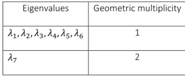
Appling Eq. (22) to Eq. (68) knowing λi with i = 1…7, the geometric multiplicities are summarized in the Table 2.
Table 2. Geometric multiplicity (or number of Jordan block) for each eigenvalue of A. Eigenvalues Geometric multiplicity
𝜆1, 𝜆2, 𝜆3, 𝜆4, 𝜆5, 𝜆6 1
𝜆7 2
14 2 dim ker(𝐴 − 𝜆𝑖. 𝐼)𝑗− dim ker(𝐴 − 𝜆𝑖. 𝐼)𝑗+1− dim ker(𝐴 − 𝜆𝑖. 𝐼)𝑗−1 (23) Using the relation Eq. (23), the number of Jordan blocks are summarize as:
- one block of size four and one block of size two for 𝑃1(𝜆) eigenvalues - each 𝑃2(𝜆) eigenvalues have one block of size one
Then, the general form of the matrix J is provided such as:
𝐽 =⊕𝑖𝐽𝑗(𝜆𝑖) (24)
where ⊕ is the direct sum and J is a squared matrix, called the Jordan normal form of A for a given eigenvalue λi, with the form:
𝐽𝑖 = [ 𝜆𝑖 1 0 0 0 𝜆𝑖 ⋱ 0 ⋮ ⋱ ⋱ 1 0 ⋯ 0 𝜆𝑖 ] (25)
The combination of Eq. (24) with Eq. (25) gives:
𝐽 = 𝐽1(𝜆1) ⊕ 𝐽1(𝜆2) ⊕ 𝐽1(𝜆3) ⊕ 𝐽1(𝜆4) ⊕ 𝐽1(𝜆5) ⊕ 𝐽1(𝜆6) ⊕ 𝐽4(𝜆7) ⊕ 𝐽2(𝜆7) (26) The matrix 𝐽 is similar to a block diagonal matrix as:
𝐽 = [ 𝐽1(𝜆1) 0 0 0 0 0 0 0 0 𝐽1(𝜆2) 0 0 0 0 0 0 0 0 𝐽1(𝜆3) 0 0 0 0 0 0 0 0 𝐽1(𝜆4) 0 0 0 0 0 0 0 0 𝐽1(𝜆5) 0 0 0 0 0 0 0 0 𝐽1(𝜆6) 0 0 0 0 0 0 0 0 𝐽4(𝜆7) 0 0 0 0 0 0 0 0 𝐽2(𝜆7)] (27)
The exponential part of Eq. (20) becomes:
𝑒𝐽.𝑥= [ 𝑒𝐽1(𝜆1).𝑥 0 0 0 0 0 0 0 0 𝑒𝐽1(𝜆2).𝑥 0 0 0 0 0 0 0 0 𝑒𝐽1(𝜆3).𝑥 0 0 0 0 0 0 0 0 𝑒𝐽1(𝜆4).𝑥 0 0 0 0 0 0 0 0 𝑒𝐽1(𝜆5).𝑥 0 0 0 0 0 0 0 0 𝑒𝐽1(𝜆6).𝑥 0 0 0 0 0 0 0 0 𝑒𝐽4(𝜆7).𝑥 0 0 0 0 0 0 0 0 𝑒𝐽2(𝜆7).𝑥] (28)
As explained previously, the Jordan blocks Ji corresponding to λi respectively take the shape λi.I + N where N (nilpotent matrix) is defined such as 𝑁𝑖,𝑗= 𝛿𝑖,𝑗+1 (δ is the Kronecker delta) and I is the
15 identity matrix. This form is the Jordan-Chevalley decomposition [46, 47]. Using the nilpotent matrix properties and Eq. (17), Eq. (28) becomes:
𝑒𝐽.𝑥= [ 𝑒𝜆1.𝑥 0 0 0 0 0 0 0 0 0 0 0 0 𝑒𝜆2.𝑥 0 0 0 0 0 0 0 0 0 0 0 0 𝑒𝜆3.𝑥 0 0 0 0 0 0 0 0 0 0 0 0 𝑒𝜆4.𝑥 0 0 0 0 0 0 0 0 0 0 0 0 𝑒𝜆5.𝑥 0 0 0 0 0 0 0 0 0 0 0 0 𝑒𝜆6.𝑥 0 0 0 0 0 0 0 0 0 0 0 0 1 𝑥 𝑥2 2 𝑥3 6 0 0 0 0 0 0 0 0 0 1 𝑥 𝑥2 2 0 0 0 0 0 0 0 0 0 0 1 𝑥 0 0 0 0 0 0 0 0 0 0 0 1 0 0 0 0 0 0 0 0 0 0 0 0 1 𝑥 0 0 0 0 0 0 0 0 0 0 0 1] (29)
The resolution of the eigenvector problem Eq. (30) for each 𝑃1(𝜆) eigenvalues leads to the set Eq. (31).
𝐴. 𝑣𝑖 = 𝜆𝑖. 𝑣𝑖 (30)
𝑉1= {𝑣1, 𝑣2, 𝑣3, 𝑣4, 𝑣5, 𝑣6} (31)
Jordan chains provide the eigenvectors set of each Jordan block [48]. The generalized eigenvector relation is:
𝑥𝑗 = (𝐴 − 𝜆. 𝐼)𝑚−𝑗. 𝑥
𝑚 𝑤𝑖𝑡ℎ 𝑥𝑚 ∈ ker(𝐴 − 𝜆. 𝐼)𝑚 (32) where 𝑚 is the Jordan block size and 𝑗 is the vector index. Using the relation Eq. (32), the eigenvector of a Jordan block of size four and two are respectively:
𝑉2= {𝐴3. 𝑥
4, 𝐴2. 𝑥4, 𝐴. 𝑥4, 𝑥4} 𝑤𝑖𝑡ℎ 𝑥4∈ ker 𝐴4 (33)
𝑉3= {𝐴. 𝑥2, 𝑥2} 𝑤𝑖𝑡ℎ 𝑥2∈ ker 𝐴2 (34)
The concatenation of those three vector sets leads to the 𝑃 invertible matrix building as:
𝑃 = [𝑉1, 𝑉2, 𝑉3] (35)
A transformation from the complex space ℂ to real space ℝ manages complex eigenvalues and eigenvectors. The transformation is applied for two conjugate complex numbers named respectively 𝜆𝑘 and 𝜆𝑘. For each line 𝑗 of an eigenvector 𝑞𝑘 (respectively 𝑞𝑘+1= 𝑞̅̅̅) linked to an eigenvalue 𝜆𝑘 𝑘 (respectively 𝜆𝑘+1= 𝜆̅̅̅): 𝑘
16 {𝑓𝑘(𝑥) = 𝑞𝑗,𝑘𝑒 𝜆𝑘.𝑥= (𝑞𝑗,𝑘0+ 𝑖. 𝑞𝑗,𝑘∗)𝑒𝜆𝑘0.𝑥[cos(𝜆𝑘∗. 𝑥) + 𝑖. sin(𝜆𝑘∗. 𝑥)] 𝑓𝑘+1(𝑥) = 𝑞̅̅̅̅̅𝑒𝑗,𝑘 𝜆𝑘.𝑥= (𝑞𝑗,𝑘0− 𝑖. 𝑞𝑗,𝑘∗)𝑒𝜆𝑘 0.𝑥 [cos(𝜆𝑘∗. 𝑥) − 𝑖. sin(𝜆𝑘∗. 𝑥)] (36) where:
- 𝜆𝑘0and 𝑞𝑗,𝑘0 are respectively the real part of 𝜆𝑘 and 𝑞𝑘,𝑗 - 𝜆𝑘∗ and 𝑞𝑗,𝑘∗ are respectively the imaginary part of 𝜆𝑘 and 𝑞𝑘,𝑗 The transformation gives:
{𝑔𝑘(𝑥) = 1
2(𝑓𝑘(𝑥) + 𝑓𝑘+1(𝑥)) = 𝑅𝑒(𝑓𝑘(𝑥)) = 𝑅𝑒(𝑓𝑘+1(𝑥)) 𝑔𝑘+1(𝑥) =12(𝑓𝑘(𝑥) − 𝑓𝑘+1(𝑥)) = 𝐼𝑚(𝑓𝑘(𝑥)) = −𝐼𝑚(𝑓𝑘+1(𝑥))
(37)
Using Eq. (37) and Eq. (74) in Eq. (29) leads to the following final expression:
1 0 0 0 0 0 0 0 0 0 0 0 1 0 0 0 0 0 0 0 0 0 0 0 0 1 0 0 0 0 0 0 0 0 0 0 0 1 0 0 0 0 0 0 0 0 0 0 2 1 0 0 0 0 0 0 0 0 0 6 2 1 0 0 0 0 0 0 0 0 0 0 0 0 . cos . sin 0 0 0 0 0 0 0 0 0 0 . sin . cos 0 0 0 0 0 0 0 0 0 0 0 0 . cos . sin 0 0 0 0 0 0 0 0 0 0 . sin . cos 0 0 0 0 0 0 0 0 0 0 0 0 0 0 0 0 0 0 0 0 0 0 0 0 2 3 2 . . . . . . . . . . . x x x x x x x x t e x t e x t e x t e x t e x t e x t e x t e e e e x s x s x s x s x s x s x s x s x r x r x J (38)Relations Eq. (77) and Eq. (30) leads to the following general eigenvector expression:
𝑣𝑘(𝜆𝑘) = [ 1 𝑣21 𝑣31+ 𝑣34𝑣41 𝑣41 𝜆𝑘 𝜆𝑘𝑣21 𝜆𝑘(𝑣31+ 𝑣34𝑣41) 𝜆𝑘𝑣41 𝜆𝑘2(𝑣 31+ 𝑣34𝑣41) 𝜆𝑘2𝑣 41 𝜆𝑘3(𝑣31+ 𝑣34𝑣41) 𝜆𝑘3𝑣 41 ] (39) where:
17 { 𝑣21= (−𝐴𝐴12) 𝑣31= (𝐺2𝑒𝐴1 𝑎𝑏𝑒1𝜆𝑘− 2 𝑒1𝜆𝑘− 2𝐴1 𝑒1𝐴2𝜆𝑘) 𝑣34= (−𝑒2 𝑒1) 𝑣34𝑣4 𝑣41= 𝐸𝑎𝑏 𝑒𝐷1𝑣31−𝐺𝑎𝑏𝑒12𝑒𝐷1𝜆𝑘(1−𝑣21)−𝐺𝑎𝑏𝑒1 2 4𝑒𝐷1𝜆𝑘2𝑣31+𝜆𝑘4𝑣31 𝐸𝑎𝑏 𝑒𝐷1(1−𝑣34)+𝐺𝑎𝑏𝑒14𝑒𝐷1𝜆𝑘2(𝑒2+𝑒1𝑣34)−𝜆𝑘4𝑣34 (40)
and vk is the eigenvector linked to the eigenvalue λk. Substituting eigenvalue calculated previously and by using Eq. (37), the last set of vector V1 is expressed as:
𝑉1= {𝑣1(𝑅1), 𝑣2(𝑅2), 𝑅𝑒(𝑣3(𝑅3)), 𝐼𝑚(𝑣3(𝑅3)), 𝑅𝑒(𝑣5(𝑅5)), 𝐼𝑚(𝑣5(𝑅5))} (41) The relationships in Eq. (39) and Eq. (41) finally provide the final P matrix by concatenation as:
𝑃 = [𝑉1, 𝑉2, 𝑉3] (42)
The solution generated by this method is used to build the K stiffness matrix. Finally, using Eqs. (20), (38), and (42), the nodal displacements and forces are then obtained with Eq. (10) leading to the stiffness matrix with Eq. (11).
3.3. Results
The final matrix computed with the aforementioned method was compared to the one provided by [27, 28]. Each stiffness matrix component computed with this new method are strictly the same as those computed with the earlier method [27, 28]. As a result, the use of the ME formulated with the new method of resolution leads to the same predictions as with the use of the earlier formulation. The accuracy of the ME model by itself has already been extensively assessed on the case of the Single Lap Joint in previous published papers [27–30, 49, 50]. Thus, more validations on the linear elastic SLJ case is not necessary. Therefore, in the next section, the linear elastic DLJ case will be explored with the presented approach. With this method, it is easier to address solution of ME governing equations and to keep flexibility on the initial formulation by always using the same resolution technique. The generation of new ME is then more straightforward.
18 In this section, a formulation of a multi-layered ME is described. This generalized formulation cover particular cases of SLJ and DLJ. Firstly, the whole formulation is described. Secondly, a particular case, corresponding to DLJ, is studied.
4.1. Formulation
The basis for the formulation is the same than in the previous section. As a result, the hypotheses and associated limitations are the same as described in section 2.1. However, there is an additional one: a linear shear stress variation in the adherend thickness following [16]. This hypothesis will be named TOM. The ME is made of a total of P adherends (or layers). A total number of P - 1 adhesive layers (or interfaces) are then involved. Two types of equilibrium are considered at the same time for the ME formulation. The first one named GR type from [9] and the second named HS type from [10–12]. The HS type takes into consideration the adhesive thickness in the local equilibrium bending equation contrary to the GR type. To deal with these two cases, the following function is introduced:
ℎ𝑖,𝑗𝑝 = ℎ𝑖+ 𝑝ℎ𝑗′ (43)
where 𝑝 is the switching condition:
- If p = 0, then the equilibrium is under GR type - If p = 1, then the equilibrium is under HS type
and where hi is the half-thickness of the adherend i such as ℎ𝑖 =
𝑒𝑖
2 and hj’ of the half-thickness of the adhesive j such as ℎ𝑗′=
𝑡𝑗
2 where ei and tj are respectively the thickness of the adherend and the adhesive. The local equilibrium of an isolated portion dx of a multi-layered element (Fig. 3) provides the following set of equations:
{
𝑑𝑁1 𝑑𝑥 + 𝑇1𝑏 = 0 𝑑𝑉1 𝑑𝑥 − 𝑆1. 𝑏 = 0 𝑑𝑀1 𝑑𝑥 + 𝑉1+ 𝑇1𝑏ℎ1,1 𝑝 = 0 (44)19 { 𝑑𝑁𝑖 𝑑𝑥 − (𝑇𝑖−1− 𝑇𝑖)𝑏 = 0 𝑑𝑉𝑖 𝑑𝑥 + (𝑆𝑖−1− 𝑆𝑖). 𝑏 = 0 𝑑𝑀𝑖 𝑑𝑥 + 𝑉𝑖+ (𝑇𝑖−1ℎ𝑖,𝑖−1 𝑝 + 𝑇 𝑖ℎ𝑖,𝑖𝑝)𝑏 = 0 𝑤𝑖𝑡ℎ 2 ≤ 𝑖 ≤ 𝑃 − 1 (45) { 𝑑𝑁𝑃 𝑑𝑥 − 𝑇𝑃−1𝑏 = 0 𝑑𝑉𝑃 𝑑𝑥 + 𝑆𝑃−1. 𝑏 = 0 𝑑𝑀𝑃 𝑑𝑥 + 𝑉𝑃+ 𝑇𝑃−1𝑏ℎ𝑃,𝑃−1 𝑝 = 0 (46)
The adhesive is considered linear elastic and as raised previously, simulated by an infinite number of elastic shear and peel springs. The adhesive spring relations are:
{
𝑆𝑖= 𝑘𝐼,𝑖[
𝑣𝑖− 𝑣𝑖+1]
𝑇𝑖 = 𝑘𝐼𝐼,𝑖
[
𝑢𝑖+1− 𝑢𝑖− ℎ𝑖+1𝜃𝑖+1 − ℎ𝑖𝜃𝑖]
(47) with 1 ≤ i ≤ P-1, where kI,i and kII,i are respectively the peel and shear rigidity and hi the half-thickness of the layer i. For an adherend i, ui is the longitudinal displacement, vi the transversal displacement and θi the bending angle.20 Figure 3. Free body diagram of the 1st, ith and Pth adherends under 1D-beam kinematics.
The constitutive equations considering a shear stress variation in the thickness are [27, 28]:
{
𝑁1= 𝐴1𝑑𝑢1 𝑑𝑥 − 𝐵1 𝑑𝜃1 𝑑𝑥 −𝐻
1 𝑑𝑇1 𝑑𝑥 𝑀1= −𝐵1𝑑𝑢1 𝑑𝑥 + 𝐷1 𝑑𝜃1 𝑑𝑥 +𝐾
1 𝑑𝑇1 𝑑𝑥 𝜃1= 𝑑𝑣1 𝑑𝑥 (48)21 { 𝑁𝑖 = 𝐴𝑖𝑑𝑢𝑑𝑥𝑖− 𝐵𝑖𝑑𝜃𝑑𝑥𝑖−
𝐻
𝑖𝑑𝑇𝑑𝑥𝑖−1−𝐻
𝑖′ 𝑑𝑇𝑑𝑥𝑖 𝑀𝑖= −𝐵𝑖𝑑𝑢𝑑𝑥𝑖+ 𝐷𝑖𝑑𝜃𝑑𝑥𝑖+𝐾
𝑖𝑑𝑇𝑑𝑥𝑖−1+𝐾
𝑖′ 𝑑𝑇𝑑𝑥𝑖 𝜃𝑖 =𝑑𝑣𝑖 𝑑𝑥 𝑤𝑖𝑡ℎ 2 ≤ 𝑖 ≤ 𝑃 − 1 (49) { 𝑁𝑃 = 𝐴𝑃𝑑𝑢𝑑𝑥𝑃− 𝐵𝑃𝑑𝜃𝑑𝑥𝑃−𝐻
𝑃′ 𝑑𝑇𝑑𝑥𝑃−1 𝑀𝑃= −𝐵𝑃𝑑𝑢𝑃 𝑑𝑥 + 𝐷𝑃 𝑑𝜃𝑃 𝑑𝑥 +𝐾
𝑃 ′ 𝑑𝑇𝑃−1 𝑑𝑥 𝜃𝑃 =𝑑𝑣𝑑𝑥𝑃 (50) where, for 1 ≤ i ≤ P:{
𝐻𝑖= 1 2𝐺𝑖(
𝐵𝑖− 1 2ℎ𝑖𝐷𝑖)
𝐻′𝑖= 1 2𝐺𝑖(
𝐵𝑖+ 1 2ℎ𝑖𝐷𝑖)
(51){
𝐾𝑖= 1 2𝐺𝑖(
𝐷𝑖− 1 2ℎ𝑖𝐹𝑖)
𝐾′𝑖= 1 2𝐺𝑖(
𝐷𝑖+ 1 2ℎ𝑖𝐹𝑖)
(52){
𝐴𝑖 = 𝑏∑
𝑄𝑖𝑝𝑖(
ℎ𝑝 𝑖− ℎ𝑝𝑖−1)
𝑛𝑖 𝑝𝑖=1 𝐵𝑖 =𝑏 2∑
𝑄𝑖 𝑝𝑖(
ℎ 𝑝𝑖2− ℎ𝑝𝑖−12)
𝑛𝑖 𝑝𝑖=1 𝐷𝑖 =𝑏 3∑
𝑄𝑖 𝑝𝑖(
ℎ 𝑝𝑖3− ℎ𝑝𝑖−13)
𝑛𝑖 𝑝𝑖=1 𝐹𝑖= 𝑏 4∑
𝑄𝑖 𝑝𝑖(
ℎ 𝑝𝑖4− ℎ𝑝𝑖−14)
𝑛𝑖 𝑝𝑖=1 (53)where Ai is the membrane stiffness, Bi is the coupling membrane-bending stiffness, Di is the bending stiffness, Gi is the Coulomb’s modulus, and Qipi is the matrix of reduced stiffness in the pith ply of the adherend i. As in the previous section, the system can be written as:
𝑑𝑌 𝑑𝑥
= 𝐴. 𝑌
(54) with:{
𝑌 = [𝑢 𝑣
𝑑𝑢𝑑𝑥 𝑑𝑣𝑑𝑥 𝑑𝑥𝑑2𝑣2 𝑑𝑑𝑥3𝑣3]
𝑇 𝑑𝑌 𝑑𝑥= [
𝑑𝑢 𝑑𝑥 𝑑𝑣 𝑑𝑥 𝑑2𝑢 𝑑𝑥2 𝑑2𝑣 𝑑𝑥2 𝑑3𝑣 𝑑𝑥3 𝑑4𝑣 𝑑𝑥4]
𝑇𝑢 = [𝑢
1… 𝑢
𝑃]
𝑣 = [𝑣
1… 𝑣
𝑃]
(55)22 In the frame of a 1D-beam kinematics, there are three degree of freedom (dof) per node. Therefore, one ME of P layers has a total of 6(P+1) dof. As a result, A is a square 6(P+1) x 6(P+1) matrix, and Y is a column vector of size 6(P+1).
4.2 Particular cases
The SLJ is the particular case of P = 2. If p = 0 for Eq. (43) it leads to GR type. Supposing Hi = Hi’ = Ki = Ki’ = 0 with 1 ≤ i ≤ P, the set of equations provided by Eqs. (44) – (52) is the same than Eq. (1) – (3). The
DLJ (Fig. 4) is the particular case of P = 3. Assuming p = 0 for Eq. (43), the set of equations provided by Eqs. (44), (45), and (46) becomes:
{
𝑑𝑁1 𝑑𝑥 + 𝑇1𝑏 = 0 𝑑𝑉1 𝑑𝑥 − 𝑆1. 𝑏 = 0 𝑑𝑀1 𝑑𝑥 + 𝑉1+ 𝑇1𝑏ℎ1,1 1 = 0 (56) { 𝑑𝑁2 𝑑𝑥 − (𝑇1− 𝑇2)𝑏 = 0 𝑑𝑉2 𝑑𝑥 + (𝑆1− 𝑆2). 𝑏 = 0 𝑑𝑀2 𝑑𝑥 + 𝑉2+ (𝑇1ℎ2,1 1 + 𝑇 2ℎ2,21 )𝑏 = 0 (57) { 𝑑𝑁3 𝑑𝑥 − 𝑇2𝑏 = 0 𝑑𝑉3 𝑑𝑥 + 𝑆2. 𝑏 = 0 𝑑𝑀3 𝑑𝑥 + 𝑉3+ 𝑇2𝑏ℎ3,2 1 = 0 (58) Eq. (47) becomes:{
𝑆1 = 𝑘𝐼,1[
𝑣1− 𝑣2]
𝑇1 = 𝑘𝐼𝐼,1[
𝑢2− 𝑢1− ℎ2𝜃2− ℎ1𝜃1]
𝑆2 = 𝑘𝐼,2[
𝑣2− 𝑣3]
𝑇2 = 𝑘𝐼𝐼,2[
𝑢3− 𝑢2− ℎ3𝜃3− ℎ2𝜃2]
(59) where:23 { 𝑘𝐼,1=𝐸𝑡𝑎11 𝑘𝐼𝐼,1=𝐺𝑎1 𝑡1 𝑘𝐼,2=𝐸𝑡𝑎2 2 𝑘𝐼𝐼,2=𝐺𝑎2 𝑡2 (60)
Assuming Hi = Hi’ = Ki = Ki’ = 0 with 1 ≤ i ≤ P and Bi = 0, the constitutive equations become, from Eqs. (48), (49), and (50):
{
𝑁1= 𝐴1𝑑𝑢1 𝑑𝑥 𝑀1= 𝐷1𝑑𝜃1 𝑑𝑥 𝜃1= 𝑑𝑣1 𝑑𝑥 (61) { 𝑁2= 𝐴2𝑑𝑢𝑑𝑥2 𝑀2= 𝐷2𝑑𝜃2 𝑑𝑥 𝜃2=𝑑𝑣𝑑𝑥2 (62) { 𝑁3 = 𝐴3𝑑𝑢𝑑𝑥3 𝑀3= 𝐷3𝑑𝜃3 𝑑𝑥 𝜃3=𝑑𝑣𝑑𝑥3 (63) Eq. (55) becomes:{
𝑌 = [𝑢 𝑣
𝑑𝑢𝑑𝑥 𝑑𝑣𝑑𝑥 𝑑𝑥𝑑2𝑣2 𝑑𝑑𝑥3𝑣3]
𝑇 𝑑𝑌 𝑑𝑥= [
𝑑𝑢 𝑑𝑥 𝑑𝑣 𝑑𝑥 𝑑2𝑢 𝑑𝑥2 𝑑2𝑣 𝑑𝑥2 𝑑3𝑣 𝑑𝑥3 𝑑4𝑣 𝑑𝑥4]
𝑇𝑢 = [𝑢
1𝑢
2𝑢
3]
𝑣 = [𝑣
1𝑣
2𝑣
3]
(64)After some simplification, Eq. (64) becomes:
{
𝑌 = [
𝑢1 𝑢2 𝑢3 𝑣1 𝑣2 𝑣3 𝑑𝑢1 𝑑𝑥 𝑑𝑢2 𝑑𝑥 𝑑𝑢3 𝑑𝑥 𝑑𝑣1 𝑑𝑥 𝑑𝑣2 𝑑𝑥 𝑑𝑣3 𝑑𝑥 𝑑2𝑣1 𝑑𝑥2 𝑑2𝑣2 𝑑𝑥2 𝑑2𝑣3 𝑑𝑥2 𝑑3𝑣1 𝑑𝑥3 𝑑3𝑣2 𝑑𝑥3 𝑑3𝑣3 𝑑𝑥3]
𝑇 𝑑𝑌 𝑑𝑥= [
𝑑𝑢1 𝑑𝑥 𝑑𝑢2 𝑑𝑥 𝑑𝑢3 𝑑𝑥 𝑑𝑣1 𝑑𝑥 𝑑𝑣2 𝑑𝑥 𝑑𝑣3 𝑑𝑥 𝑑2𝑢1 𝑑𝑥2 𝑑2𝑢2 𝑑𝑥2 𝑑2𝑢3 𝑑𝑥2 𝑑2𝑣1 𝑑𝑥2 𝑑2𝑣2 𝑑𝑥2 𝑑2𝑣3 𝑑𝑥2 𝑑3𝑣1 𝑑𝑥3 𝑑3𝑣2 𝑑𝑥3 𝑑3𝑣3 𝑑𝑥3 𝑑4𝑣1 𝑑𝑥4 𝑑4𝑣2 𝑑𝑥4 𝑑4𝑣3 𝑑𝑥4]
𝑇 (65)Finally, Eq. (54) becomes: 𝑑𝑌
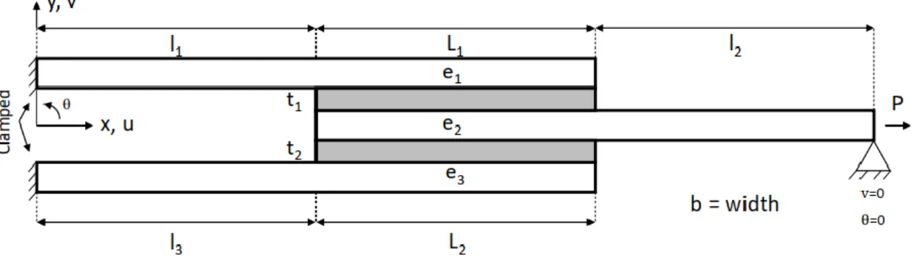
24 with A, a square matrix provided in Appendix B. Thanks to the aforementioned, the general analytical solution of the system is determined where the characteristic polynomial is 18th order. It owns eight conjugate, four real and six null eigenvalues. Therefore, the nodal displacements and forces are determined. Then, the stiffness matrix K is computed. The free adherends are modeled as traditional Euler-Bernoulli laminated beam. For a symmetrical DLJ (Fig. 4), the properties used are listed in the Table 3. On one side, it is clamped and on the other side, loaded with a force P = 100 N.
Figure 4. Double lap joint annotation.
Table 3. Double lap joint properties.
Adherend 1 𝑒1= 2 mm 𝑏 = 10 mm 𝑙1= 100 mm 𝐸1= 70 GPa 𝜈1= 0.33 Adhesive 1 𝑡1 = 250 µm 𝑏 = 10 mm 𝐿1= 30 mm 𝐸𝑎1= 2240 MPa 𝐺𝑎1= 800 MPa Adherend 2 𝑒2= 2 mm 𝑏 = 10 mm 𝑙2= 100 mm 𝐸2= 70 GPa 𝜈2= 0.33 Adhesive 2 𝑡2= 250 µm 𝑏 = 10 mm 𝐿2= 30 mm 𝐸𝑎2= 2240 GPa 𝐺𝑎2= 800 MPa Adherend 3 𝑒3= 2 mm 𝑏 = 10 mm 𝑙3= 100 mm 𝐸3= 70 GPa 𝜈3= 0.33
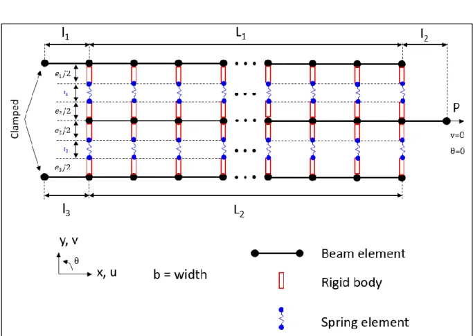
A 1D FE models has been built with beam elements for the adherends and spring elements for the adhesive layer, to be as close as possible to the ME modelling hypothesis. The nodes associated with beam elements are located at the actual neutral line of adherends. The nodes associated with the spring elements are located at the actual interfaces of adherends. For each adherend along the overlap, rigid body elements were used to link the nodes of the neutral lines and to the nodes of the adherend interface. A scheme of the 1D FE model used is provided in Fig. 5. Beam elements are based
25 on degree 3 interpolating functions under the Euler-Bernoulli kinematics. The overlap length of adherends was then regularly meshed with the number of ME (nBE). This parameter has been set to 600. The springs stiffnesses kui and kvi are directly related to the mesh density along the overlap [51]. For a spring element located at an abscissa x along the overlap, the stiffnesses are computed from the value of adhesive peel and shear modulus, the adhesive thicknesses t1 or t2, the width b and the mesh density 𝑛𝐿 𝐵𝐸 such as: { 𝑘𝑣1(𝑥) = 𝑚(𝑥)𝑛𝐿𝐵𝐸𝑏𝐸𝑡𝑎11 = 𝑚(𝑥)𝑛𝐿𝐵𝐸𝑏𝑘𝐼,1 𝑘𝑢1(𝑥) = 𝑚(𝑥)𝑛𝐿 𝐵𝐸𝑏 𝐺𝑎1 𝑡1 = 𝑚(𝑥) 𝐿 𝑛𝐵𝐸𝑏𝑘𝐼𝐼,1 𝑘𝑣2(𝑥) = 𝑚(𝑥)𝑛𝐿 𝐵𝐸𝑏 𝐸𝑎2 𝑡2 = 𝑚(𝑥) 𝐿 𝑛𝐵𝐸𝑏𝑘𝐼,2 𝑘𝑢2(𝑥) = 𝑚(𝑥)𝑛𝐿 𝐵𝐸𝑏 𝐺𝑎2 𝑡2 = 𝑚(𝑥) 𝐿 𝑛𝐵𝐸𝑏𝑘𝐼𝐼,2 (67) where 𝑚(𝑥) = { 1 2 𝑖𝑓 𝑥 = 0 𝑜𝑟 𝐿 1 𝑜𝑡ℎ𝑒𝑟𝑤𝑖𝑠𝑒
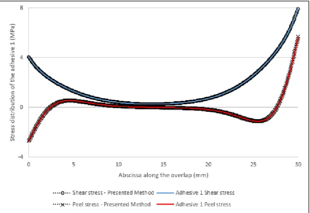
26 The peel and shear stress distribution along the overlap of each adhesive layer are respectively represented on Fig. 6 and Fig. 7.
Figure 6. DLJ symmetric - Adhesive Peel and Shear stress along the overlap of the adhesive 1 with FE model.
27 Figure 7. DLJ symmetric - Adhesive Peel and Shear stress along the overlap of the adhesive 2 with FE
model.
As expected, the adhesive stresses are symmetrical with respect to the inner adherend. In magnitude, the stresses are equal, which are expected results. Fig. 6 and Fig. 7 presents good correlation. The presented method provide equivalent results than the 1D FE model. The maximum absolute error observed here is 0.1% along the overlap compared to the range of stress values. For a dissimilar DLJ (Fig. 4), the properties used are listed in the Table 4. Boundaries conditions are the same than previously. The peel and shear stress distribution along the overlap of each adhesive layer are respectively represented on Fig. 8 and Fig. 9.
Table 4. Dissimilar Double Lap Joint properties.
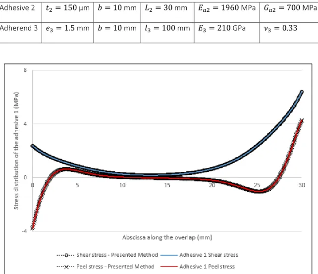
Adherend 1 𝑒1= 2 mm 𝑏 = 10 mm 𝑙1= 100 mm 𝐸1= 70 GPa 𝜈1= 0.33 Adhesive 1 𝑡1 = 250 µm 𝑏 = 10 mm 𝐿1= 30 mm 𝐸𝑎1= 2240 MPa 𝐺𝑎1= 800 MPa Adherend 2 𝑒2= 2.5 mm 𝑏 = 10 mm 𝑙2= 100 mm 𝐸2= 65 GPz 𝜈2= 0.33
28 Adhesive 2 𝑡2= 150 µm 𝑏 = 10 mm 𝐿2= 30 mm 𝐸𝑎2= 1960 MPa 𝐺𝑎2= 700 MPa Adherend 3 𝑒3= 1.5 mm 𝑏 = 10 mm 𝑙3= 100 mm 𝐸3= 210 GPa 𝜈3= 0.33
Figure 8. DLJ non-symmetric - Adhesive Peel and Shear relative stress error along the overlap of the adhesive 1 with FE model.
29 Figure 9. DLJ non-symmetric - Adhesive Peel and Shear stress along the overlap of the adhesive 2 with
FE model.
As expected, the aforementioned method can deal with non-symmetrical geometry. The Fig. 8 and Fig. 9 presents good correlation. The presented method provide equivalent results than the 1D FE model. The maximum absolute error observed here is 0.1% along the overlap compared to the range of stress values.
5. Conclusion
Numerous models based on various sets of simplifying hypotheses exist to provide, at low computational time, accurate predictions of the mechanical behavior of bonded aircraft structures at the presizing stage. If closed-form solutions can sometimes be derived, the use of dedicated resolution schemes is mainly required to solve the system of ODEs coming from the simplifying hypotheses. The ME technique is one of these dedicated resolution schemes. It is based on the formulation the stiffness matrix of specific 4-nodes element to model a bonded overlap. The original methodology for the formulation of ME allows for the providing of the shape of solutions in terms of adherend
30 displacements and internal loads [24–28]. The direct consequence is that only one ME is needed to model the full length of the bonded overlap and then to obtain the distributions of adherend displacements and internal forces as well as the adhesive stresses at any abscissa of the overlap. However, it is difficult with the original method to take into account some variations in the set of simplifying hypotheses. A second methodology, making use of the exponential matrix, has then been suggested to quickly formulate the ME stiffness matrix when the simplifying hypotheses are modified [31, 32]. Nevertheless, the shape of solutions for the adherend displacements and internal force are not known anymore, so that the results are only available at nodes. It means that a dedicated mesh is required to post-process the result at any abscissa. In the present paper, a new methodology for the formulation of ME stiffness matrices is presented. This methodology offers the ability to easily take into account for the modification of simplifying hypotheses while providing the shape of solutions, which reduced then the computational time. The system of ODEs is solved using the Jordan form approach. This methodology is illustrated on the SLJ configuration step by step. The results provided are the same as those provided by the original approach by in terms of adhesive stresses. The methodology is then applied to formulate a multi-layered ME involving various local equilibrium equations and constitutive equations. This multi-layered ME is then illustrated on a DLJ configuration under a 1D-beam kinematics. In both illustrations, good results with 1D FE models have been obtained. The aforementioned method is a turnkey method for first order ODEs system with constant coefficients. On a different ODEs type, it has to be adapted. The use of Euler-Bernoulli beam model to model the adherends is not a restriction and other beam models, such as Timoshenko one, could be considered in the frame of this methodology. Finally, the presented research in this paper focus on the derivation of solution shapes of displacement field, in order to take benefit from the ME technique. The formulation methodology can be easily applied – and implemented in the computer code – from various sets of simplified hypotheses, chosen to describe at best the mechanical behavior of the bonded structure under consideration. This approach can be employed to model structural joining areas in-plane loaded or considered as mainly in-plane loaded, which exhibit complex geometries.
31 These areas can involve fasteners [30]. They can be subjected to a variation of temperature, making use of the equivalent nodal force approach available in the FE method [32]. Finally, nonlinear material behaviors can be supported by an analysis based on a dedicated iterative procedure as presented in [29, 30].
Acknowledgments
The author affiliated to Sogeti High Tech gratefully acknowledges the engineers and the managers involved in the development of JoSAT (Joint Stress Analysis Tool), which is an internal research program. The authors warmly acknowledge Mr Salah Seddiki2 for the supplying of FE predictions.
Declarations of interest None.
Appendixes. A. Single Lap Joint
A1. Differential equation resolution
The system Eq. (8) leads to the following characteristic polynomial:
{ 𝑃(𝑅) = 𝑃1(𝑅) ∗ 𝑃2(𝑅) 𝑃1(𝑅) = 𝑅3 𝑃2(𝑅) = 𝑅3+ 𝑘 1𝑅2+ 𝑘2𝑅 + 𝑘3 (68) where: { 𝑅 = 𝜆2 𝑘1= −𝐺𝑏𝑒 (𝐴1 1+ 1 𝐴2+ 𝑒12 4𝐷1+ 𝑒22 4𝐷2) 𝑘2=𝐸𝑏 𝑒 ( 1 𝐷1+ 1 𝐷2) 𝑘3= −𝐸𝐺𝑏2 𝑒2 [ 1 𝐴1𝐷1+ 1 𝐴2𝐷1+ 1 𝐴1𝐷2+ 1 𝐴2𝐷2+ (𝑒1+𝑒2)2 4𝐷1𝐷2 ] (69)
Looking for root square 𝑅 of 𝑃(𝑅) in Eq. (68) is equivalent to the separated problem 𝑃1(𝑅) and 𝑃2(𝑅). 𝑃1(𝑅) and 𝑃2(𝑅) have respectively 3 null (named 𝑅4) and 3 non-null eigenvalues (named 𝑅1, 𝑅2, 𝑅3).
32 Using the first relation from Eq. (69), 𝑅𝑖 with 𝑖 ∈ [1,4] provides 6 null (named 𝜆7) and 6 non-nul eigenvalues (named 𝜆𝑖 with 𝑖 ∈ [1,6]). Cardan’s method is used to determinate 𝑃2(𝑅) eigenvalues of Eq. (68) by rewriting it as:
𝑃2(𝑅′) = 𝑅′3+ 𝑝̂𝑅′+ 𝑞̂ (70) where: { 𝑅′= 𝑅 −𝑘31 𝑅 = 𝜆2 𝑝̂ = −𝑘12 3 + 𝑘2 𝑞̂ = −𝑘1 27(2𝑘12− 9𝑘2) + 𝑘3 Δ̂ = 27𝑞̂2+ 4𝑝̂3 (71)
According to the sign of the Cardan’s discriminant, three specific cases can be distinguished: (i) Δ > 0, (ii) Δ = 0 and (iii) Δ < 0. Each case leads to a set {𝑅1, 𝑅2, 𝑅3} of eigenvalue of 𝑃2(𝑅) and then to the set {𝜆1, 𝜆2, 𝜆3, 𝜆4, 𝜆5, 𝜆6} of eigenvalues of 𝑃2(𝜆). In a single lap joint (SLJ) problem, the most common case is the positive Cardan’s discriminant [13]. The Cardan’s discriminant solutions are:
{ 𝑅1′ = 𝑢 + 𝑣 = 𝑟2−𝑘31 𝑅2′ = 𝑗. 𝑢 + 𝑗̅. 𝑣 = (𝑠 + 𝑖. 𝑡)2−𝑘1 3 𝑅3′ = 𝑗2. 𝑢 + 𝑗̅ . 𝑣 = (𝑠 − 𝑖. 𝑡)2 2−𝑘1 3 (72) where: { 𝑢 = √−𝑞̂+√Δ̂/27 2 3 𝑣 = √3 −𝑞̂−√Δ2̂/27 𝑗 = 𝑗̅ = −2 1 2+ 𝑖 √3 2 𝑗2= 𝑗̅ = −1 2− 𝑖 √3 2 (73)
and where “ i ” refers to the imaginary unit so that 𝑖2= −1. Depending on the sign of the roots {𝑅1′, 𝑅2′, 𝑅3′}, the six roots {𝑅1, 𝑅2, 𝑅3, 𝑅4, 𝑅5, 𝑅6} of the characteristic polynomial can be defined using Eqs. (72) and (73) as:
𝑅1= +𝑟 𝑅2= −𝑟 𝑅3= (𝑠 + 𝑖𝑡) 𝑅4= (𝑠 − 𝑖𝑡) 𝑅5= −(𝑠 + 𝑖𝑡) 𝑅6= −(𝑠 − 𝑖𝑡) (74) Or:
33 𝑅1= +𝑖𝑟 𝑅2 = −𝑖𝑟 𝑅3= (𝑠 + 𝑖𝑡) 𝑅4= (𝑠 − 𝑖𝑡) 𝑅5= −(𝑠 + 𝑖𝑡) 𝑅6= −(𝑠 − 𝑖𝑡) (75) depending on the sign of 𝑅1′ in Eq. (72). Therefore, the adhesive shear and peel stress expressions are:
{
𝑆(𝑥) = [𝐾̅̅̅𝑒1 𝑠.𝑥sin(𝑡. 𝑥) + 𝐾̅̅̅𝑒2 𝑠.𝑥cos(𝑡. 𝑥) + 𝐾̅̅̅𝑒3 −𝑠.𝑥sin(𝑡. 𝑥) +𝐾̅̅̅𝑒4 −𝑠.𝑥cos(𝑡. 𝑥) + 𝐾̅̅̅𝑒5 𝑟.𝑥+ 𝐾̅̅̅𝑒6 −𝑟.𝑥 ] 𝑇(𝑥) = [𝐾1𝑒𝑠.𝑥+𝐾sin(𝑡. 𝑥) + 𝐾2𝑒𝑠.𝑥cos(𝑡. 𝑥) + 𝐾3𝑒−𝑠.𝑥sin(𝑡. 𝑥)
4𝑒−𝑠.𝑥cos(𝑡. 𝑥) + 𝐾5𝑒𝑟.𝑥+ 𝐾6𝑒−𝑟.𝑥+ 𝐾7 ]
(76)
where 𝐾̅ with 𝑗 ∈ [1,6] and 𝐾𝑗 𝑗 with 𝑗 ∈ [1,7] are integration constants, which can be expressed as combinations of ci with 𝑖 ∈ [1,12] from Eq. (9). By combining Eqs. (1), (5), and (76), the nodal displacements and forces are expressed to compute Eq. (10) which provides the stiffness matrix with Eq. (11).
A2. Matrix representation
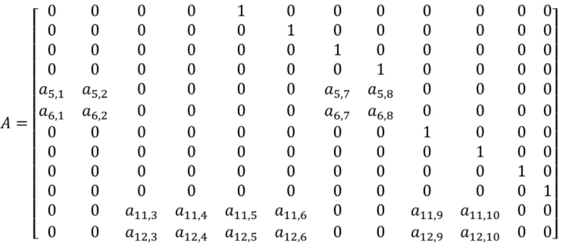
The square matrix A used in Eq. (15) is the following:
𝐴 = [ 0 0 0 0 1 0 0 0 0 0 0 0 0 0 0 0 0 1 0 0 0 0 0 0 0 0 0 0 0 0 1 0 0 0 0 0 0 0 0 0 0 0 0 1 0 0 0 0 𝑎5,1 𝑎5,2 0 0 0 0 𝑎5,7 𝑎5,8 0 0 0 0 𝑎6,1 𝑎6,2 0 0 0 0 𝑎6,7 𝑎6,8 0 0 0 0 0 0 0 0 0 0 0 0 1 0 0 0 0 0 0 0 0 0 0 0 0 1 0 0 0 0 0 0 0 0 0 0 0 0 1 0 0 0 0 0 0 0 0 0 0 0 0 1 0 0 𝑎11,3 𝑎11,4 𝑎11,5 𝑎11,6 0 0 𝑎11,9 𝑎11,10 0 0 0 0 𝑎12,3 𝑎12,4 𝑎12,5 𝑎12,6 0 0 𝑎12,9 𝑎12,10 0 0] (77)
The components of the matrix A in Eq. (25) are given in Table A-1.
Table A-1. Constant expression of Eq. (77) 𝑎5,1= 𝐺𝑏 𝑒𝐴1 𝑎5,2= − 𝐺𝑏 𝑒𝐴1 𝑎5,7=𝐺𝑏𝑒1 2𝑒𝐴1 𝑎5,8=𝐺𝑏𝑒2 2𝑒𝐴1 𝑎6,1= − 𝐺𝑏 𝑒𝐴2 𝑎6,2= 𝐺𝑏 𝑒𝐴2 𝑎6,7= −𝐺𝑏𝑒1 2𝑒𝐴2 𝑎6,8= −𝐺𝑏𝑒2 2𝑒𝐴2 𝑎11,3= − 𝐸𝑏 𝑒𝐷1 𝑎11,5= 𝐺𝑏𝑒1 2𝑒𝐷1 𝑎11,9= 𝐺𝑏𝑒12 4𝑒𝐷1
34 𝑎11,4= 𝐸𝑏 𝑒𝐷1 𝑎11,6= − 𝐺𝑏𝑒1 2𝑒𝐷1 𝑎11,10 = 𝐺𝑏𝑒1𝑒2 4𝑒𝐷1 𝑎12,3= 𝐸𝑏 𝑒𝐷2 𝑎12,4= − 𝐸𝑏 𝑒𝐷2 𝑎11,5= 𝐺𝑏𝑒2 2𝑒𝐷2 𝑎11,6= − 𝐺𝑏𝑒2 2𝑒𝐷2 𝑎11,9= 𝐺𝑏𝑒1𝑒2 4𝑒𝐷2 𝑎11,10 =𝐺𝑏𝑒2 2 4𝑒𝐷2
B. Double lap joint matrix coefficients
By combining Eqs. (56), (59), (61), and (62), it comes: 𝑑2𝑢1 𝑑𝑥2 = ( 𝑏𝐺𝑎1 A1𝑡1) 𝑢1+ (− 𝑏𝐺𝑎1 A1𝑡1) 𝑢2+ ( 𝑏𝐺𝑎1𝑒1 2A1𝑡1) 𝑑𝑤1 𝑑𝑥 + ( 𝑏𝐺𝑎1𝑒2 2A1𝑡1) 𝑑𝑤2 𝑑𝑥 𝑑4𝑤 1 𝑑𝑥4 = ( 𝑏𝑒1𝐺𝑎1 2𝑡1D1) 𝑑𝑢1 𝑑𝑥 + (− 𝑏𝑒1𝐺𝑎1 2𝑡1D1) 𝑑𝑢2 𝑑𝑥 + (− 𝑏𝐸𝑎1 𝑡1D1) 𝑤1+ ( 𝑏𝐸𝑎1 𝑡1D1) 𝑤2+ ( 𝑏𝑒12𝐺𝑎1 4𝑡1D1) 𝑑2𝑤 1 𝑑𝑥2 + ( 𝑏𝑒1𝑒2𝐺𝑎1 4𝑡1D1 ) 𝑑2𝑤 2 𝑑𝑥2 such as: 𝑑2𝑢 1 𝑑𝑥2 = 𝑘1𝑢1+ 𝑘2𝑢2+ 𝑘3 𝑑𝑤1 𝑑𝑥 + 𝑘4 𝑑𝑤2 𝑑𝑥 𝑑4𝑤 1 𝑑𝑥4 = 𝑘15 𝑑𝑢1 𝑑𝑥 + 𝑘16 𝑑𝑢2 𝑑𝑥 + 𝑘17𝑤1+ 𝑘18𝑤2+ 𝑘19 𝑑2𝑤 1 𝑑𝑥2 + 𝑘20 𝑑2𝑤 2 𝑑𝑥2
By combining Eqs. (57), (59), (61), (62), and (63), it comes: 𝑑2𝑢2 𝑑𝑥2 = (− 𝑏𝐺𝑎1 A2𝑡1) 𝑢1+ ( 𝑏𝐺𝑎1 A2𝑡1+ 𝑏𝐺𝑎2 A2𝑡2) 𝑢2+ (− 𝑏𝐺𝑎2 A2𝑡2) 𝑢3+ (− 𝑏𝐺𝑎1𝑒1 2A2𝑡1) 𝑑𝑤1 𝑑𝑥 + (− 𝑏𝐺𝑎1𝑒2 2A2𝑡1 + 𝑏𝐺𝑎2𝑒2 2A2𝑡2) 𝑑𝑤2 𝑑𝑥 + (𝑏𝐺𝑎2𝑒3 2A2𝑡2) 𝑑𝑤3 𝑑𝑥 𝑑4𝑤 2 𝑑𝑥4 = ( 𝑏𝑒2𝐺𝑎1 2𝑡1D2) 𝑑𝑢1 𝑑𝑥 + ( 𝑏𝑒2𝐺𝑎2 2𝑡2D2 − 𝑏𝑒2𝐺𝑎1 2𝑡1D2) 𝑑𝑢2 𝑑𝑥 + (− 𝑏𝑒2𝐺𝑎2 2𝑡2D2) 𝑑𝑢3 𝑑𝑥 + ( 𝑏𝐸𝑎1 𝑡1D2) 𝑤1+ (− 𝑏𝐸𝑎1 𝑡1D2− 𝑏𝐸𝑎2 𝑡2D2) 𝑤2+ (𝑏𝐸𝑎2 𝑡2D2) 𝑤3+ ( 𝑏𝑒1𝑒2𝐺𝑎1 4𝑡1D2 ) 𝑑2𝑤1 𝑑𝑥2 + ( 𝑏𝑒22𝐺𝑎1 4𝑡1D2 + 𝑏𝑒22𝐺𝑎2 4𝑡2D2) 𝑑2𝑤2 𝑑𝑥2 + ( 𝑏𝑒2𝑒3𝐺𝑎2 4𝑡2D2 ) 𝑑2𝑤3 𝑑𝑥2 such as: 𝑑2𝑢2 𝑑𝑥2 = 𝑘5𝑢1+ 𝑘6𝑢2+ 𝑘7𝑢3+ 𝑘8 𝑑𝑤1 𝑑𝑥 + 𝑘9 𝑑𝑤2 𝑑𝑥 + 𝑘10 𝑑𝑤3 𝑑𝑥 𝑑4𝑤2 𝑑𝑥4 = 𝑘21 𝑑𝑢1 𝑑𝑥 + 𝑘22 𝑑𝑢2 𝑑𝑥 + 𝑘23 𝑑𝑢3 𝑑𝑥 + 𝑘24𝑤1+ 𝑘25𝑤2+ 𝑘26𝑤3+ 𝑘27 𝑑2𝑤1 𝑑𝑥2 + 𝑘28 𝑑2𝑤2 𝑑𝑥2 + 𝑘29 𝑑2𝑤3 𝑑𝑥2
By combining Eqs. (58), (59), (63), and (64), it comes: 𝑑2𝑢 3 𝑑𝑥2 = (− 𝑏𝐺𝑎2 A3𝑡2) 𝑢2+ ( 𝑏𝐺𝑎2 A3𝑡2) 𝑢3+ (− 𝑏𝐺𝑎2𝑒2 2A3𝑡2) 𝑑𝑤2 𝑑𝑥 + (− 𝑏𝐺𝑎2𝑒3 2A3𝑡2) 𝑑𝑤3 𝑑𝑥
35 𝑑4𝑤3 𝑑𝑥4 = ( 𝑏𝑒3𝐺𝑎2 2𝑡2D3) 𝑑𝑢2 𝑑𝑥 + (− 𝑏𝑒3𝐺𝑎2 2𝑡2D3) 𝑑𝑢3 𝑑𝑥 + ( 𝑏𝐸𝑎2 𝑡2D3) 𝑤2+ (− 𝑏𝐸𝑎2 𝑡2D3) 𝑤3+ ( 𝑏𝑒2𝑒3𝐺𝑎2 4𝑡2D3 ) 𝑑2𝑤2 𝑑𝑥2 + ( 𝑏𝑒32𝐺𝑎2 4𝑡2D3) 𝑑2𝑤3 𝑑𝑥2 such as: 𝑑2𝑢3 𝑑𝑥2 = 𝑘11𝑢2+ 𝑘12𝑢3+ 𝑘13 𝑑𝑤2 𝑑𝑥 + 𝑘14 𝑑𝑤3 𝑑𝑥 𝑑4𝑤 3 𝑑𝑥4 = 𝑘30 𝑑𝑢2 𝑑𝑥 + 𝑘31 𝑑𝑢3 𝑑𝑥 + 𝑘32𝑤2+ 𝑘33𝑤3+ 𝑘34 𝑑2𝑤 2 𝑑𝑥2 + 𝑘35 𝑑2𝑤 3 𝑑𝑥2
The square matrix A is then expressed as:
𝐴 = [ 0 0 0 0 0 0 𝑘1 𝑘5 0 0 0 0 0 0 0 0 0 0 0 0 0 0 0 0 𝑘2 𝑘6 𝑘11 0 0 0 0 0 0 0 0 0 0 0 0 0 0 0 0 𝑘7 𝑘12 0 0 0 0 0 0 0 0 0 0 0 0 0 0 0 0 0 0 0 0 0 0 0 0 𝑘17 𝑘24 0 0 0 0 0 0 0 0 0 0 0 0 0 0 0 0 𝑘18 𝑘25 𝑘32 0 0 0 0 0 0 0 0 0 0 0 0 0 0 0 0 𝑘26 𝑘33 1 0 0 0 0 0 0 0 0 0 0 0 0 0 0 𝑘15 𝑘21 0 0 1 0 0 0 0 0 0 0 0 0 0 0 0 0 𝑘16 𝑘22 𝑘30 0 0 1 0 0 0 0 0 0 0 0 0 0 0 0 0 𝑘23 𝑘31 0 0 0 1 0 0 𝑘3 𝑘8 0 0 0 0 0 0 0 0 0 0 0 0 0 0 1 0 𝑘4 𝑘9 𝑘13 0 0 0 0 0 0 0 0 0 0 0 0 0 0 1 0 𝑘10 𝑘14 0 0 0 0 0 0 0 0 0 0 0 0 0 0 0 0 0 0 1 0 0 0 0 0 𝑘19 𝑘27 0 0 0 0 0 0 0 0 0 0 0 1 0 0 0 0 𝑘20 𝑘28 𝑘34 0 0 0 0 0 0 0 0 0 0 0 1 0 0 0 0 𝑘29 𝑘35 0 0 0 0 0 0 0 0 0 0 0 0 1 0 0 0 0 0 0 0 0 0 0 0 0 0 0 0 0 0 0 1 0 0 0 0 0 0 0 0 0 0 0 0 0 0 0 0 0 0 1 0 0 0] (78)
where ki with 1 ≤ i ≤ 35 are constants described previously.
REFERENCES
[1]
Hart-Smith, L. J. Technical Report AFWAL-TR-81-3154, (1982).
[2]
Higgins, A. Int. J. Adhes. Adhes. 20 (5), 367–376 (2000). DOI:
10.1016/S0143-7496(00)00006-3.
[3]
Kelly, G. Compos. Struct. 72 (1), 119–129 (2006). DOI:
10.1016/j.compstruct.2004.11.002.
[4]
da Silva, LFM, Öschner, A, Adams, RD (Editors), 2018. Handbook of Adhesion
Technology (2 volumes), 2nd edition Springer: Heidelberg, Germany.
[5]
van Ingen, J.W., and Vlot, A. Report LR-740, (1993).
[6]
Tsai, M. Y., and Morton, J. Int. J. Solids Struct. 31 (18), 2537–2563 (1994). DOI:
10.1016/0020-7683(94)90036-1.
[7]
da Silva, L. F. M., das Neves, P. J. C., Adams, R. D., and Spelt, J. K. Int. J. Adhes.
Adhes. 29 (3), 319–330 (2009). DOI: 10.1016/j.ijadhadh.2008.06.005.
[8]
Volkersen, O. Luftfahrtforschung. 15 (24), 41–47 (1938).
[9]
Goland, M., and Reissner, E. J. Appl. Mech. 11, A17–A27 (1944).
[10] Hart-Smith, L. J. NASA Technical Report CR112237, (1973).
[11] Hart-Smith, L. J. NASA Technical Report CR112236, (1973).
[12] Hart-Smith, L. J. NASA Technical Report CR112235, (1973).
36