Mid-level sparse representations for timbre identification: design of an instrument-specific harmonic dictionary

HAL Id: inria-00544284

https://hal.inria.fr/inria-00544284

Submitted on 7 Dec 2010

HAL is a multi-disciplinary open access

archive for the deposit and dissemination of

sci-entific research documents, whether they are

pub-lished or not. The documents may come from

teaching and research institutions in France or

abroad, or from public or private research centers.

L’archive ouverte pluridisciplinaire HAL, est

destinée au dépôt et à la diffusion de documents

scientifiques de niveau recherche, publiés ou non,

émanant des établissements d’enseignement et de

recherche français ou étrangers, des laboratoires

publics ou privés.

identification: design of an instrument-specific harmonic

dictionary

Pierre Leveau, Emmanuel Vincent, Gael Richard, Laurent Daudet

To cite this version:

Pierre Leveau, Emmanuel Vincent, Gael Richard, Laurent Daudet. Mid-level sparse representations

for timbre identification: design of an instrument-specific harmonic dictionary. 1st Workshop on

Learning the Semantics of Audio Signals (LSAS), Dec 2006, Athens, Greece. �inria-00544284�

Mid-level sparse representations for timbre

identification:

design of an instrument-specific harmonic

dictionary

†_{GET/ENST, 37-39 rue Dareau, 75014 Paris – France}

‡_{LAM (Universit´e Pierre et Marie Curie), 11, rue de Lourmel, 75015 Paris – France} ?_{Centre for Digital Music, Queen Mary, Univ. of London, London E1 4NS – UK}

Abstract

Several studies have pointed out the need of mid-level representations of music signals for information retrieval and signal processing applica-tions. In this paper, we investigate a new representation based on sparse decomposition of the signal into a collection of instrument-specific har-monic atoms modelling notes of various pitches played by different instru-ments. Each atom is composed of windowed harmonic sinusoidal partials whose amplitudes are learned on a training database. An efficient Match-ing Pursuit algorithm was designed to extract the best atoms and to estimate the phases of their partials. Then we explain how the result-ing representation can be exploited for automatic instrument recognition. Preliminary experiments on a test database of solo excerpts show promis-ing results.

1

Introduction

Audio indexing is a field of growing interest and includes challenging goals such as automatic music transcription [1], automatic genre classification [2, 3] or mu-sic instrument recognition [4, 5, 6]. Most mumu-sic classification systems so far are based on a set of timbral and temporal features computed from low-level signal representations, such as waveforms, spectrograms or correlograms. These features, which describe the signal as a whole on each time frame, do not ac-count for all the attributes of complex polyphonic signals. By contrast, the human auditory system is generally able to assess the timbre of each note or the rhythm of each instrument separately. It is expected that the decomposition of the signal into a collection of musically meaningful sound objects could help au-tomatic systems achieving a similar performance. For example, several authors have designed mid-level representations of music signals in terms of note-like

objects extracted using complex polyphonic pitch transcription algorithms and proved their benefit for various applications, namely auditory scene analysis [7], recognition of multiple instruments [8, 9], measurement of harmonic similarity [10] and source separation [11].

In this paper, we investigate a new mid-level representation of music signals based on the concept of sparse decomposition. Sparse decomposition methods have received a lot of attention recently in signal processing and approximation theory communities. Their aim is to provide a representation (exact or approxi-mate) of a given signal x as a linear combination of fixed elementary waveforms, or atoms: x(t) = N X n=1 αnwn(t) (1)

where atoms wn are selected among a set D = {wn}n=1...P, called a dictionary.

Audio signals are typically modelled using Gabor atoms, which are sinusoids windowed by Gaussian envelopes, and whose time support is bounded. The term sparse refers to the property by which the number N of selected atoms is much lower than the dimension of the signal space, that is the length of the signal. When this property holds true, such decompositions can be seen as a preprocessing step for many audio signal processing operations, including coding, signal modification and information extraction [12].

Obviously, in order to get decompositions that are as sparse as possible, one has to design dictionaries that contain atoms exhibiting strong similarities with the analysed signal. Hence, the more a priori information is available on the signal, the more informed dictionaries can be designed, and the more physically meaningful the resulting decompositions are.

In the following, we assume that the analysed signal only contains sounds from harmonic instruments and that the set of possible instruments is known. Ideally, we would like to infer a MIDI-like representation of the signal, where each atom wn would represent a single note signal parameterised by an

instru-ment class, a pitch value, a velocity parameter and other expressive parameters (vibrato, etc). However, such an ideal representation cannot be obtained by sparse decomposition since the large range of possible note signals, even for a limited set of instruments, would require huge dictionaries D and result in huge computations (computational requirements directly depend on the dictionary size). Therefore, we design simpler frame-based Instrument-Specific Harmonic ISH) atoms composed of windowed harmonic sinusoidal partials whose ampli-tudes are learned on a training database for each instrument and pitch value.

In practice, some of the extracted atoms do not have a straightforward inter-pretation as notes, but are selected to correct slight discrepancies between the data and the model. Nevertheless, as we shall see, the decomposition algorithm provides an approximate representation of the signal, where the information at hand is intermediate between the raw signal and a high-level representation such as a MIDI transcription. In other words, the loss in fine details of the signal (some degradation is almost always audible) has to be balanced with the ease of interpretation of the decomposition, which includes an explicit clue about the

instruments that are playing. However, the representation with ISH atoms can-not be used directly for polyphonic transcription or source separation because these tasks need more complex priors [1]. But it comes at a smaller computa-tional cost than the more comprehensive approaches proposed in [1] and still makes possible several information retrieval tasks (key-finding, melodic similar-ity, automatic instrument recognition) and coarse remixing.

This paper focuses on the single task of automatic instrument recognition. In the scope of this application, the proposed approach shares some similari-ties with template-based instrument recognition algorithms [8, 9, 6], which also describe instrument classes in terms of learned harmonic amplitude vectors.

The structure of the rest of the paper is as follows. The ISH atoms com-posing the specific dictionary used as a signal model are defined in Section 2. Section 3 presents the algorithm used to obtain sparse decompositions on this dictionary. Section 4 describes how ISH atoms for particular instruments are learned on isolated notes. Finally, the results of automatic instrument recogni-tion experiments are shown in Secrecogni-tion 5 and commented in secrecogni-tion 6.

2

Instrument-Specific Harmonic Dictionary

The main contribution of this study is the modelling of music signals as a weighted linear combination of N harmonic atoms hsn,un,f0n,An,Φn

parame-terised in terms of scale sn (atom duration), time localisation un,

fundamen-tal frequency f0n, partials amplitudes An = {am,n}m=1:M and partials phases

Φn = {φm,n}m=1:M : x(t) = N X n=1 αnhsn,un,f0n,An,Φn(t). (2)

Each harmonic atom can be written as

hs,u,f0,A,Φ(t) = M

X

m=1

amejφmgs,u,m.f0(t) (3)

where the amplitudes of the M partials are constrained toPM_m=1a2

m= 1 and

the signal corresponding to each partial is given by a Gabor atom1 _normalised to unit energy gs,u,f = w µ t − u s ¶ e2jπf t ₍₄₎

with w a time- and frequency-localised window. For strictly speaking Gabor atoms, this window is a Gaussian, although Hanning windows are also a con-venient choice for our application. Note that harmonic atoms also have unit energy.

1_{Following the convention set in [13], atoms are denoted by complex-valued signals. In}

practice, sparse decompositions of real-valued signals involve pairs of atoms consisting of one complex-valued atom and its conjugate.

0 1000 2000 3000 4000 5000 −40 −30 −20 −10 0 10 20 30 40 62 61 A Vectors 60 59 58 Frequency [Hz] Amplitude [dB]

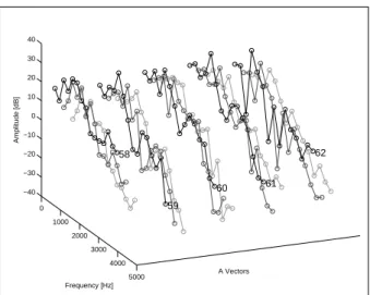
Figure 1: Examples of learned amplitude vectors A corresponding to 5 oboe notes, each played with 3 different velocities. Each partial is represented as a circle and each velocity by a different gray level. MIDI codes are displayed on the right side of the vector groups.

When partials amplitudes are learned from a database (see 4.1), these atoms are called ISH atoms. Each amplitude vector A is then associated with a class (in our case an instrument) and a discrete pitch value. Generally, several vectors are used for each class and each pitch value. Indeed, allocating a single amplitude vector to an instrument would oversimplify its timbre span: musical acousticians and synthesiser designers know that inferring a note signal by simple pitch-shifting of another note signal is not relevant for large pitch intervals. The dependency of signal characteristics on pitch has also been pointed and exploited by Kitahara [5]. Furthermore, the relative amplitudes of the partials depend on velocity and evolve over time. Examples of learned amplitude vectors A are displayed in Figure 1.

3

Decomposition algorithm

Given a ISH dictionary, the problem becomes that of decomposing the signal as a collection of ISH atoms from this dictionary. Many decomposition algorithms suited for generic dictionaries have been proposed in the literature. We have chosen Matching Pursuit (MP), as described below, for its simplicity and its relative speed due to its “greedy” nature. Although there is in general no guarantee that the N -atoms approximation obtained with MP is optimal (i.e. minimises the energy of the residual), many experiments have shown that its behaviour is generally very close to optimal, at the fraction of the time required to get more accurate approximations.

3.1

The Matching Pursuit Algorithm

The MP algorithm has been introduced in [14]. The algorithm proceeds as follows:

1. The correlations between the signal and all the atoms h of the dictionary are computed using inner products hx, hi =PT_t=1x(t) h(t).

2. The atom h that has the largest absolute correlation |hx, hi| with the signal is selected, then subtracted from the signal with a weighting coefficient

α = hx, hi.

3. Correlations are updated on the residual signal, and the algorithm is it-erated to step 2 until the stopping condition is satisfied. This condition can be a target Original-to-Residual energy ratio, or a fixed number of iterations.

3.2

Sampling the dictionary

In practical applications, the search step 2 can only be performed on a finite number of atoms. Thus, one has to sample the dictionary by making the atom parameters s,u, f0, A and Φ discrete:

– The scale s often spans a small set of powers of 2. For our application, the choice of a single scale corresponding to a duration of about 100 ms is sufficient. More scales should be chosen for other applications such as analysis-synthesis or coding (one small scale for the transients and one long scale for the steady-state part).

– The time localisation u is typically set to equally spaced time bins, with a time shift ∆u set to a fraction of the atom scale.

– The fundamental frequency f0is sampled logarithmically. This is a notice-able difference with the Harmonic MP algorithm [15], where fundamen-tal frequencies are sampled linearly. The main reason for this choice is that the distribution of fundamental frequencies in music signals appears smoother on a logarithmic scale. Thus it provides a constant f0resolution for these signals.

– Amplitude vectors A are by nature elements of a discrete set of vectors, because they are learnt from a finite number of sound excerpts. The building of this set is described in section 4. The number of amplitude vectors per class and pitch value must not be too large for computational reasons. This point is discussed in section 4.1.

– A brute-force sampling of phase vectors Φ would be very expensive in terms of complexity, since this would multiply the size of the dictionary by (2π/∆φ)M_{, where ∆φ is the phase bin width. Alternatively, phase}

3.3

Phase estimation

At each iteration of the MP algorithm, the partials phases of the selected atom must be adapted to the analysed signal. Otherwise the subtraction of this atom may add energy to some partials and result in the extraction of spurious atoms during later iterations. The phase vector is thus given by the angle of the inner product between the Gabor atoms constituting the ISH atoms and the signal:

ejφm ₌ hx, gs,u,m.f0i

|hx, gs,u,m.f0i|. (5)

This method can be shown to be nearly optimal for strongly sinusoidal signals when the Gabor atoms gs,u,m.f0 are sufficiently uncorrelated (this is the case

when s and/or f0 are large enough) [15].

4

Learning on isolated notes

The amplitude vectors A corresponding to various classes and pitch values are learned on a training database. The choice of the number of vectors and the choice of the learning database both influence the cost and the relevance of the decomposition.

4.1

Training database

In this study, the training database is composed of isolated note signals taken from the RWC Musical Instrument Sound Database [16] for five instruments: Oboe, Flute, Clarinet, Violin and Cello. These signals span the whole pitch range of each instrument and correspond to three different velocities. We extract one amplitude vector A per note signal. This results in a small number of amplitude vectors for each class and each pitch value. However the fact that these vectors are learnt from different velocities lets us expect that they span a significant part of each instrument timbre. There are between 100 and 200 different A vectors per instrument (between 3 and 6 per pitch and instrument).

4.2

Partial amplitude extraction

To keep a certain homogeneity between learning and signal decomposition, the amplitude amof each partial is extracted by computing the absolute value of the

inner product between the training signal and a Gabor atom of frequency m.f0. The annotated fundamental frequency f0 given by its integer MIDI pitch does not exactly correspond to the true fundamental frequency, especially for bowed strings instruments. This problem is solved as follows: harmonic combs of Gabor atoms, sampled at a fine fundamental frequencies f0around the annotated pitch, are correlated with the signal. The best fundamental frequency f0n is selected

by: f0n= arg max f0 M X m=1 |hxn, gs,u,m.f0i|2. (6)

The amplitude of each partial is then derived as:

am,n= |hxn, gs,u,m.f0ni|. (7)

5

Application to automatic instrument

recogni-tion

5.1

Output of the signal decomposition

The “informed” sparse decomposition described in section 3 can be considered has a front-end for some applications. The result of the MP algorithm is a

book of atoms that can be displayed on a time-pitch plane, along with other

characteristics such as overall energy and instrument class.

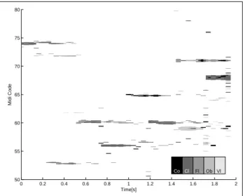
The decomposition of a real solo music signal is displayed in figure 2. It is important to note that this analysed signal is not part of the training database. Reconstructed sounds can be listened to on our web page2_{. Some interesting} features can be observed. In particular, the atoms can be visually grouped as clusters corresponding to certain pitch values. Thus the mid-level structure of the analysed signal as a collection of notes seems to be very well represented.

0 0.2 0.4 0.6 0.8 1 1.2 1.4 1.6 1.8 2 50 55 60 65 70 75 80 Time[s] Midi Code Co Cl Fl Ob Vl

Figure 2: Time-pitch visualisation of the decomposition of a clarinet recording. Each atom is represented by a rectangle whose height is proportional to its amplitude and whose colour depends on its instrument class.

As mentionned in introduction, the proposed model is too simple to be used directly for polyphonic transcription or source separation. Here we evaluate its usefulness for the task of automatic instrument recognition on monophonic signals: this application can be easily performed. Indeed it is expected that

the atoms that are selected in this case mainly belong to the instrument that is playing.

5.2

Decision procedure

One way of achieving automatic instrument recognition is to compute a score for each instrument class by summing the amplitudes |αn| of all the extracted

atoms from this class. In the case of a solo performance, the instrument with the largest score is then the most likely to be played.

6

Experiments

6.1

Parameters

The decomposition algorithm has been applied on a test database of solo phrases extracted from different commercial recordings, with a sampling frequency fs=

22050 Hz. The database contains 5 sources for each instrument. The total duration for each instrument is between 12 and 24 minutes. The test items are 2 second excerpts taken from these phrases. It makes between 200 and 300 test items per tested class.

The parameters used for the decomposition are the following: s = 90 ms (1024 samples), ∆u = 45 ms, maximum number of partials M = 30. The fundamental frequency f0 is sampled logarithmically with a step equal to 1/10 tone. The MP algorithm is stopped when the Original-to-Residual ratio becomes larger than 15 dB or the number of extracted atoms equal to 500.

Classification tests have also been performed with a feature-based approach that provides a good benchmark of the state-of-the-art performance on solo excerpts. The test algorithm has been developed by Essid, and is mainly based on a feature selection algorithm called Fisher-Clustering (40 features selected out of 543) and a classification with Support Vector Machine. For more details, see [4]. It must be noted that this algorithm is trained with numerous sources (solo phrases) extracted from commercial CDs, that the features also extract longer-term informations, such as amplitude- and frequency-modulations, and non-harmonic characteristics, while our algorithm is trained on isolated notes from a single source and only considers the harmonic part of the signal. For that reason, the two systems cannot be strictly compared: the feature-based approach only gives a first goal to reach.

The feature-based approach is performed on the same test samples than the signal analysed in the decompositions. The decisions are taken on the frames contained in 2 seconds of signal (125 test frames).

6.2

Results

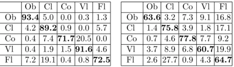
The confusion matrices obtained from the various algorithms are shown in Table 1. The feature-based algorithm appears quite robust, with an overall recognition

accuracy of 83.9%. The proposed algorithm achieves an average recognition rate of 68.5 % using books obtained directly after the decomposition.

Although not comparable with the feature-based approach, the application of our decomposition algorithm to automatic instrument recognition shows an interesting feature: the recognition accuracy is higher for the Cello class. This is certainly related to the explicit modelling of the instrument pitch range: Cello has a lower pitch range than the other instruments, and thus low notes are automatically detected as Cello notes.

Ob Cl Co Vl Fl Ob 93.4 5.0 0.0 0.3 1.3 Cl 4.2 89.2 0.9 0.0 5.7 Co 0.4 7.4 71.7 20.5 0.0 Vl 0.4 1.9 1.5 91.6 4.6 Fl 7.2 19.1 0.4 0.8 72.5 Ob Cl Co Vl Fl Ob 63.6 3.2 7.3 9.1 16.8 Cl 1.4 75.8 3.9 1.8 17.1 Co 0.7 4.6 77.8 7.7 9.2 Vl 3.7 8.9 6.8 60.7 19.9 Fl 2.6 27.7 0.9 4.3 64.7

Table 1: Confusion matrix for instrument recognition with a state-of-the-art feature based approach(left), and based on decompositions on ISH atoms (right).

7

Conclusion

In this paper, a novel approach for music signal analysis is proposed. It is based on sparse decompositions of the audio signal using instrument-specific harmonic atoms extracted from real recordings. The preliminary results obtained in a mu-sic instrument recognition task are very promising even if they do not yet reach the performances of more traditional approaches. In fact, it is important to note that this alternative approach has the potential to perform simultaneously instrument recognition, polyphonic pitch transcription and source separation. Future work will be dedicated to the use of smoothing techniques for the selec-tion of atoms with time (for example based on dynamic programming principles which should permit to explicitly build coherent group of atoms, or molecules) and to the design of optimal dictionaries (with the aim to maximise the cov-erage of the acoustic space for the given instrument while at the same time minimising its size). Future work will also be dedicated to the application of this approach to more complex tasks such as instrument recognition and pitch extraction on polyphonic music signals, by introducing more complex priors for atom selection.

8

Acknowledgements

This work has been partially supported by the K-SPACE Network of Excellence, the French CNRS and EPSRC grant GR/S75802/01. The first author wishes to thank the Centre for Digital Music at Queen Mary, University of London, for welcoming him and providing the possibility to have fruitful discussions

with Emmanuel Vincent and other researchers, including Mark Plumbley, Mark Sandler, Juan Bello and Thomas Blumensath. R´emi Gribonval, who was visiting the Centre, also gave a very interesting enlightening for this work. Many thanks to Slim Essid for giving us the results of his automatic instrument recognition algorithm.

References

[1] A. Klapuri and M. Davy, editors. Signal Processing Methods for Music

Transcription. Springer, New York, NY, 2006.

[2] G. Tzanetakis and P. Cook. Musical Genre Classification of Audio Signals.

IEEE Trans. on Speech and Audio Processing, 10(5):293, 2002.

[3] T. Li and M. Ogihara. Music genre classification with taxonomy. In IEEE, editor, Proc. of ICASSP, 2005.

[4] S. Essid, G. Richard, and B. David. Musical instrument recognition by pair-wise classification strategies. IEEE Trans. on Audio, Speech and Language

Processing, 2006.

[5] T. Kitahara, M. Goto, K. Komatani, T. Ogata, and H.G. Okuno. In-strument identification in polyphonic music: feature weighting with mixed sounds, pitch-dependent timber modeling, and use of musical context. In

Proc. ISMIR, 2005.

[6] J. Eggink and G. J. Brown. Instrument recognition in accompanied sonatas and concertos. In Proc. of ICASSP, 2004.

[7] D.P.W. Ellis. Prediction-driven computational auditory scene analysis. PhD thesis, MIT, 1996.

[8] K. Kashino and H. Murase. A sound source identification system for en-semble music based on template adaptation and music stream extraction.

Speech Communication, 27:337–349, 1999.

[9] T. Kinoshita, S. Sakai, and H. Tanaka. Musical sound source identification based on frequency component adaptation. In Proc. IJCAI Worshop on

CASA, pages 18–24, 1999.

[10] J. Pickens, J.P. Bello, G. Monti, T. Crawford, M. Dovey, M. Sandler, and D. Byrd. Polyphonic score retrieval using polyphonic audio queries: A harmonic modeling approach. In Proc. ISMIR, pages 140–149, 2002. [11] E. Vincent. Musical source separation using time-frequency source priors.

IEEE Trans. on Audio, Speech and Language Processing, 14(1):91–98, 2006.

[12] L. Daudet and B. Torr´esani. Sparse adaptive representations for musical signals. In Signal Processing Methods for Music Transcription. Springer, may 2006.

[13] R. Gribonval. Fast matching pursuit with a multiscale dictionary of gaus-sian chirps. IEEE Trans. on Signal Processing, 49(5):994–1001, 2001. [14] S. Mallat and Z. Zhang. Matching pursuits with time-frequency

dictionar-ies. IEEE Trans. on Signal Processing, 41(12):3397–3415, 1993.

[15] R. Gribonval and E. Bacry. Harmonic decomposition of audio signals with matching pursuit. IEEE Trans. on Signal Processing, 51(1):101–111, 2003. [16] M. Goto, H. Hashiguchi, T. Nishimura, and R. Oka. RWC Musical Instrument Sound Database. Distributed online at http://staff.aist.go.jp/m.goto/RWC-MDB/.