CONTRÔLE ENVIRONNEMENTAL DE LA STRUCTURE
ET DE LA DISTRIBUTION DE LA COMMUNAUTÉ
MICROBIENNE DANS LE GOLFE DE SAN JORGE,
ARGENTINE
ENVIRONMENTAL CONTROL OF THE STRUCTURE AND DISTRIBUTION OF THE MICROBIAL COMMUNITY IN THE GULF OF SAN JORGE, ARGENTINA
Mémoire présentée
dans le cadre du programme de maîtrise en océanographie en vue de l’obtention du grade de maître en science
PAR
© MAITÉ PILMAYQUEN LATORRE Juin 2018
Composition du jury :
Michel Gosselin, président du jury, Université du Québec à Rimouski
Gustavo A. Ferreyra, directeur de recherche, Université du Québec à Rimouski, CADIC
Irene R. Schloss, codirectrice de recherche, CADIC
Lemarchand, Karine, codirectrice de recherche, Université du Québec à Rimouski Gaston Almandoz, codirecteur de recherche, Universidad Nacional de la Plata CONICET
Michel Starr, examinateur externe, Institute Maurice-Lamontagne
UNIVERSITÉ DU QUÉBEC À RIMOUSKI Service de la bibliothèque
Avertissement
La diffusion de ce mémoire ou de cette thèse se fait dans le respect des droits de son auteur, qui a signé le formulaire « Autorisation de reproduire et de diffuser un rapport, un mémoire ou une thèse ». En signant ce formulaire, l’auteur concède à l’Université du Québec à Rimouski une licence non exclusive d’utilisation et de publication de la totalité ou d’une partie importante de son travail de recherche pour des fins pédagogiques et non commerciales. Plus précisément, l’auteur autorise l’Université du Québec à Rimouski à reproduire, diffuser, prêter, distribuer ou vendre des copies de son travail de recherche à des fins non commerciales sur quelque support que ce soit, y compris l’Internet. Cette licence et cette autorisation n’entraînent pas une renonciation de la part de l’auteur à ses droits moraux ni à ses droits de propriété intellectuelle. Sauf entente contraire, l’auteur conserve la liberté de diffuser et de commercialiser ou non ce travail dont il possède un exemplaire.
À ma mère Adriana Nill et à mon père Victor Latorre, qui m'ont semé la curiosité par la mer.
REMERCIEMENTS
J'aimerais remercier l'expérience que m’apporté vivre à Rimouski. Dans ce petit endroit j'ai d'abord rencontré la neige, puis la chaleur des gens qui y vivent.
Je voudrais surtout remercier l'État d’Argentine qui, par le biais du programme BEC.AR m'a attribué une bourse pour réaliser cette maîtrise. Ma gratitude va aussi aux institutions, à l'Université du Québec à Rimouski et à l'ISMER, qui ont cordialement reçus l’ensemble des boursiers Argentines, répondant à tous nos besoins, grâce à des bourses, des programmes d'apprentissage du français et tout le matériel nécessaire pour réaliser mon travail de recherche.
Je tiens à remercier tout particulièrement mes directeurs Gustavo Ferreyra, Irene Schloss, Karine Lemarchand et Gaston Almandoz pour m'avoir accompagné tout au long du processus, m'enseignant les techniques de traitement des données, m'aidant à interpréter les résultats et à écrire ce présent mémoire. Je voudrais également remercier Gustavo et Irene de m’avoir accueillie en famille, de m’avoir écouter et de m’avoir soutenir dans les moments les plus difficiles.
Je tiens à remercier "Les Filles", Juli, Xime, Elo et Ary, ce petit groupe d'Argentines rêveur et fort. Ça n'aurait pas été pareil sans vous. Merci pour les mates et les promenades au beau Québec.
Merci à mes colocs, qui ont été nombreux et chacun m'a donné de beaux souvenirs, de différentes histoires et la chaleur humaine pour me sentir comme chez moi. Pour Mymy, Jean et Arthur, j'espère que nous nous reverrons quelque part.
À Catty, Mary-Ann et Catty! Merci pour la belle « maison jeune », les fêtes et les randonnées à la plage.
A ma famille qui m’accompagne pendant tout le processus et m’encourager à suivre mes rêves.
AVANT-PROPOS
Le présent travail s’inscrit dans le cadre du projet “Santé de l'écosystème marin du golfe San Jorge: état actuel et résilience” (MARES, pour son acronyme en anglais), faisant partie du projet de coopération internationale entre l'Argentine et le Québec. Ce projet a pour but d'étudier l'état actuel de l'écosystème marin du golfe de San Jorge. C’est dans ce contexte que j’ai obtenu une bourse du programme BEC.AR (Argentine) pour suivre des études de maîtrise en océanographie à l’ISMER-UQAR. Au cours de l’année 2016 j'ai reçu de l’aide financière du Service aux Étudiantes de l’UQAR afin de participer à la mission océanographique du programme Pampa Azul dans le golfe San Jorge, en Argentine. Trois présentations des résultats préliminaires ont été effectuées pendant le développement de ma maîtrise, à l’intérieur des rencontres scientifiques suivants :
• Latorre, MP, Schloss I., Almandoz G., Lemarchand K., Ferreyra G. “Environmental controls of the microbial community structure and distribution in San Jorge Gulf, Argentine”. Présentation des résultats de maîtrise. Mars 2017, Workshop PROMESse, Rimouski, Québec. Orale.
• Latorre, Maité G. Almandoz, K. Lemarchand, I.R. Schloss, G.A. Ferreyra, “Biomass distribution of the microbial community and evaluation of its physiological state in the San Jorge Gulf”, . Novembre 2016, 15e Assemblée Générale Annuelle de Québec-Océan. Affiche.
• Latorre, M.; Schloss I.; Almandoz G. ; Lemarchand K. ; Ferreyra G., "Contrôle environnemental de la structure et de la distribution de la communauté microbienne dans le Golfe de San Jorge, Argentine", Novembre 2015. 14e Assemblée Générale Annuelle de Québec-Océan. Affiche.
RÉSUMÉ
Le golfe de San Jorge (GSJ) englobe un écosystème très productif de la Patagonie argentine. Dans ce contexte, la communauté microbienne joue un rôle essentiel en générant le carbone organique qui sera consommé dans le réseau trophique marin de cette région. L'objectif de cette étude était de caractériser la composition et biomasse de la communauté microbienne et l'état physiologique du composant autotrophe en relation aux facteurs environnementaux les plus importants. L’échantillonnage a été effectuée à 16 stations à bord du R/V Coriolis II de l’Université du Québec à Rimouski, en été. La structure verticale et les courants dans la colonne d'eau ont été mesurés et des analyses chemiques et la composition et biomasse de la communauté microbienne ont été effectués. Nos résultats montrent que la température (driver primaire de la stratification dans la colonne d’eau) et les nutriments affectent la composition et distribution de la communauté. En utilisant un estimateur de la stabilité dynamique (le nombre de Richardson), il a été possible de détecter des processus turbulents dans des zones stratifiées associé à la marée et au cisaillement des masses d'eau, lesquels ont favorisé la rupture de la pycnocline. De plus, la formation de doigts de sel a été favorisé pour l’entrée des eaux de faible salinité à l'extrême sud du GSJ. Ceci suggère que les deux processus contribuent au pompage des nutriments provenant des eaux profondes à l’interface de la pycnocline, lesquels favorisent le développement de micro-phytoplancton qui soutienne des réseaux trophiques herbivores. Cependant, la communauté était dominée par le pico-plancton qui constituent des réseaux du type boucle microbienne. Le phytoplancton a toujours montré des bonnes conditions physiologiques quant à leur capacité photosynthétique. Néanmoins, la biomasse de micro-phytoplancton était toujours faible (<3 µg l-1 de carbone). L’hypothèse que nous avons tiré pour expliquer cette apparente contradiction est que l’accumulation des grandes cellules autotrophes est contrôlée par le broutage, couplé avec un haut taux de renouvellement des autotrophes. Cette hypothèse peut aussi être soutenue si l’on considère les hauts rapports du carbone vs. azote (rapport C: N, en anglais), qui suggèrent la présence d’une forte activité de broutage du zooplancton.
Mots clés : Golfe de San Jorge, Communauté microbienne, Stabilité dynamique, Nombre de Richardson, doigts de sel, Gradient de nutriments, état physiologique du phytoplancton
ABSTRACT
The San Jorge Gulf (SJG), is a highly productive ecosystem in the Patagonia Argentina. This study characterizes the base of the food web, i.e. microbial community composition, biomass and physiological state in relation with environmental factors in the SJG during summer 2014. Samples were collected at 16 stations, onboard the oceanographic vessel of the Université du Québec à Rimouski R/V Coriolis II, for which vertical structure and currents were measured. Nutrients, chlorophyll-a, dissolved oxygen, the particulate organic carbon and nitrogen and the microbial community composition and biomass were studied. Our results show that temperature (which is the main driver of stratification of the water column) and nutrients affect the distribution of the microbial community. Using a dynamic stability estimator (the Richardson number), it was possible to detect turbulent processes in stratified zones, which favored the partial disruption of the pycnocline, related to tide energy and the shear between both surface and deep-water masses. In addition, low salinity coastal waters (LSCWs) in the southern part of the gulf induce instabilities associated with density that can favor the formation of salt fingers. We have hypothesized that both processes can be pumping nutrients from deeps waters to the surface promoting the micro-phytoplankton growing, which feed herbivorous food webs with high biomass production. However, the community was dominated by pico-plankton which leads to microbial food webs or microbial loops. Additionally, the physiological state related to photosynthetic capacity of autotrophs was good, nonetheless the micro-phytoplankton size biomass was not high (<3 µg l-1 of carbon). The hypothesis that we have drawn to explain
this apparent contradiction is that the accumulation of large autotrophic cells is controlled by grazing, coupled with a high turnover rate of autotrophs. This can be supported by the high carbon vs. Nitrogen ratio (C: N ratio), which suggests the presence of a strong grazing activity by zooplankton.
Keywords: Gulf of San Jorge, Microbial community, Dynamic stability, Richardson number, Salt finger, Nutrient gradient, Physiological state of phytoplankton.
TABLE DES MATIÈRES
REMERCIEMENTS ... ix
AVANT-PROPOS ... x
RÉSUMÉ ... xi
ABSTRACT ... xii
TABLE DES MATIÈRES ... xiii
LISTE DES TABLEAUX ... xv
LISTE DES FIGURES ... xvi
LISTE DES ABRÉVIATIONS, DES SIGLES ET DES ACRONYMES ... xviii
LISTE DES SYMBOLES ... xix
INTRODUCTION GÉNÉRALE ... 1
PROBLÉMATIQUE ... 1
LACOMMUNAUTÉMICROBIENNE ... 3
ÉCHAPPERÀLABARRIÈREDELASTRATIFICATION:LESPROCESSUS DEMÉLANGEÀLAPYCNOCLINEETLEURSIMPORTANCEDANS L’APPORTDENUTRIMENTS ... 5
L’ÉTATPHYSIOLOGIQUEDUPHYTOPLANCTONETLEURRELATION AVECL’ENVIRONNEMENT... 7
OBJECTIFSETHYPOTHÈSES ... 9
CHAPITRE 1 CONTRÔLE ENVIRONNEMENTAL DE LA STRUCTURE ET DE LA DISTRIBUTION DE LA COMMUNAUTÉ MICROBIENNE DANS LE GOLFE DE SAN JORGE, ARGENTINE ... 11
1.1 CONTEXTE DU PROJET ... 11
1.2 ENVIRONMENTAL CONTROL OF THE STRUCTURE AND DISTRIBUTION OF THE MICROBIAL COMMUNITY IN THE GULF OF SAN JORGE,ARGENTINE ... 12
1.3 INTRODUCTION ... 12
1.4 MATERIALS AND METHODS ... 15
1.4.1 Sampling ... 15
1.4.2 Assessment of oceanographic conditions ... 17
1.4.3 Water column stability ... 17
1.4.4 Chemical analyses ... 19
1.4.5 Microbial community composition, abundance and biomass ... 19
1.4.5.3 Flow cytometry analyses ... 21
1.4.6 Physiological state of phytoplankton ... 22
1.4.7 Statistical analyses ... 22
1.5 RESULTS ... 23
1.5.1 General oceanographic conditions ... 23
1.5.2 Dynamic stability conditions ... 25
1.5.3 Nutrients distribution ... 27
1.5.4 Water column properties during the time series observations ... 30
1.5.5 Vertical advection of nutrients associated to dynamical stability ... 30
1.5.6 Chl-a distribution associated to oxygen concentration ... 33
1.5.7 Microbial community composition and biomass ... 35
1.5.8 Multivariable analyses ... 37
1.5.9 Chl-a integrated to the upper layer and physiological state of the autotrophic community ... 39
1.5.10 Relation between the total particulate organic carbon and community organic carbon ... 41
1.6 DISCUSSION ... 43
1.6.1 Oceanographic features in the San Jorge Gulf ... 43
1.6.2 The role of turbulence in nutrient distribution at the SJG ... 44
1.6.3 The significance of the maximum subsurface maximum Chl-a in summer. ... 47
1.6.4 Microbial community composition and physiological state in relation to environmental conditions ... 48
1.7 CONCLUSIONS ... 51
CONCLUSION GÉNÉRALE ... 53
PERSPECTIVESFUTURESDERECHERCHE ... 56
RÉFÉRENCES BIBLIOGRAPHIQUES ... 59
LISTE DES TABLEAUX
Table 1 : Density (cells L-1) of the main plankton groups classified by their size. Abbreviations means: Nano-CYAN: nanocyanobacteria, Nano-Euk: nanoeukaryotes, Pico-CYAN: picocyanobacterial, Pico-EUK: picoeukaryotes, H-BACT: heterotrophic bacteria. ... 35 Table 2: Distribution of organic carbon and nitrogen in SJG. Abbreviations means: POCT: particulate organic carbon, PONT: particulate organic nitrogen, POCT/ PONT: Organic carbon and organic nitrogen ratio, POCMC: particulate organic carbon of microbial community, POCA: particulate organic carbon of autotrophs, POCH: particulate organic carbon of heterotrophs, POCMC/POCT: ratio between microbial community and total particulate organic carbon, POCA/ POCH: ratio between autotrophs and heterotroph particulate organic carbon, POCH/ POCT: ratio between heterotrophs and total particulate organic carbon. ... 42 Table 3 : L'efficacité quantique maximale de la photochimique du PSII (Fv / Fm) dans
LISTE DES FIGURES
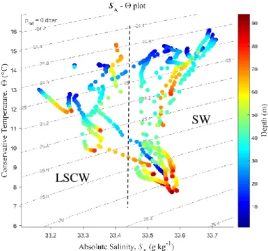
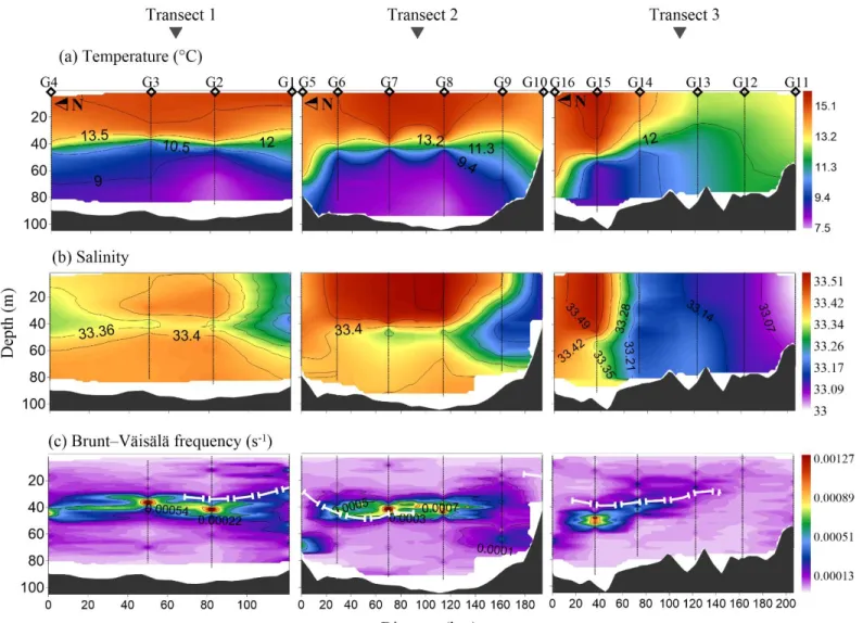
Figure 1: Study area in San Jorge Gulf (SJG). Triangles indicate location of CTD casts (G01 to G16 and FS). Doted lines indicate Transect 1, Transect 2 and Transect 3, respectively. Water (Niskin bottles) sampling stations are marked by squares (n=11). ... 16 Figure 2: Temperature-Salinity diagram showing the characteristics of the different water masses from CTD casts for all stations at SJG during summer 2014. LSCW: Low salinity coastal waters, SW: Shelf waters. ... 24 Figure 3: Vertical profiles of A) Temperature (°C), B) Salinity and C) Brunt–Väisälä frequency (s-1) in the three transects studied (Transect 1: inner gulf; Transect 2: middle gulf; Transect 3: outer gulf). White lines indicate Zeu... 26
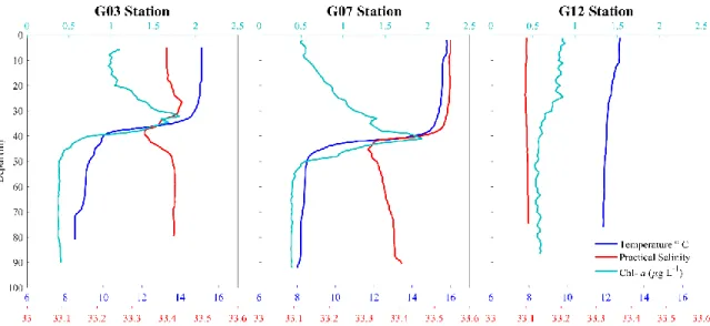
Figure 4: Vertical profiles of Temperature (º C, blue), Practical salinity (red) and Chl-a (µg L-1, green) at three stations (G03, G07 and G13) in the SJG. ... 27 Figure 5: Vertical profiles of nutrients in the three transects studied (Transect 1: inner gulf; Transect 2: middle gulf; Transect 3: outer gulf). ... 29 Figure 6: Time series at the Fixed station of a) Temperature (ºC); b) Salinity; c) Chlorophyll-a (µg L-1). Top x axes have the number of each CTD cast and bottom x axes the tidal cycle stage, where LT: Low tide; HT: High tide. White rectangles indicate the lack of data; d) Horizontal current velocity averaged in Surface waters (0-40m of depth) and in Bottom Waters (40m to the bottom). Doted lines correspond to each CTD cast. ... 31 Figure 7: Gradient of nutrients (nitrates+nitrites) (∆N/∆z) vs Richardson number (Ri) at a) Grid stations (orange dots) and fixed stations (blue dots); b) Fixed station. The dotted line shows the logarithmic relationship between both variables. ... 32 Figure 8: Vertical profiles of: a) Chl-a (µg L-1), white lines indicate Zeu;; b) Dissolved
Oxygen (ml L-1) c) Percent oxygen saturation (%) in three sections of the SJG (Transect 1: inner gulf; Transect 2: middle gulf; Transect 3: outer gulf). ... 34
Chl-a maximal depth. a) Pico-cyanobacteria; b) Pico-Eukaryotes; c) Heterotrophic bacteria; d) Ciliates; e) Diatoms, and f) Dinoflagellates. ... 36 Figure 10: Relative contribution of each size class to total carbon content of the microbial community (%). MICRO: Microplankton, NANO: Nanoplankton, PICO: Picoplankton. ... 37 Figure 11: Canonical transformation-based redundancy analysis (tb-RDA) triplot of microbial community represented in terms of carbon content (µg L-1) (red) and environmental variables (green) with samples in blue. The two first axes represent the 27% (RDA1) and 17% (RDA2) of total community variability. ... 39 Figure 12: Horizontal distribution of a) Chl-a integrated in euphotic zone (pycnocline depth); b) maximum photochemical quantum yield (Fv/Fm) at Chl-a maximal depth; c)
LISTE DES ABRÉVIATIONS, DES SIGLES ET DES ACRONYMES
Français
GSJ Golfe de San Jorge. CO2 Dioxyde de carbone.
SW Masses d'eau du plateau continental. BMW Masses d'eau de Beagle-Magellan. Chl-a Chlorophylle -a.
N Fréquence de Brunt–Väisälä.
Ri Richardson nombre.
Rp Rapport du gradient de densité. PSII Photosystème II.
Fv/Fm Maximum rendement quantique de la photochimique du PSII.
Anglais
SJG San Jorge Gulf. CO2 Carbon dioxide.
SW Shelf waters.
BMW Beagle-Magellan waters. LSCW Low salinity coastal waters. Chl-a Chlorophyll-a.
N Brunt–Väisälä frequency.
Ri Richardson number.
Fv/Fm Maximum photochemical quantum yield. Zeu Euphotic zone. DINO Dinoflagellates. DIAT Diatoms. Nano-CYAN Nanocyanobacteria. Nano-Euk Nanoeukaryotes. Pico-CYAN Picocyanobacterial. Pico-EUK Picoeukaryotes.
H-BACT Heterotrophic free bacteria. ∆N/∆z Nutrients gradient.
RDA Redundancy analysis.
Fv/Fm Maximum photochemical quantum yield. POC Particulate organic carbon.
PON Particulate organic nitrogen.
C: N Ratio between the organic carbon and nitrogen. POCMC Particulate organic carbon of microbial community. POCA Particulate organic carbon of autotrophs.
POCH Particulate organic carbon of heterotrophs.
POCMC/POCT Ratio between microbial community and total particulate organic carbon. POCA/ POCH Ratio between autotrophs and heterotroph particulate organic carbon. POCH/ POCT Ratio between heterotrophs and total particulate organic.
LISTE DES SYMBOLES Français
PSII Section efficace d'absorption du PSII. Density anomalies.
Anglais
PSII Effective absorption cross section of PSII. Anomalies de densité.
INTRODUCTION GÉNÉRALE
PROBLÉMATIQUE
Quarante pourcents de la production primaire de la planète proviennent des écosystèmes océaniques (Falkowski, 1994). Les zones les plus productives sont concentrées dans les régions côtières, telles que la plate-forme de Patagonie argentine (située dans l'Atlantique sud-ouest) qui a été identifié comme l'un des écosystèmes marins les plus importants de l'hémisphère sud (Bisbal, 1995, Gregg et al., 2005). Elle présente une productivité primaire très élevée (>300g m2an-1) (Behrenfeld et Falkowski, 1997), concentrée surtout près des zones frontales dans les talus et dans les différentes zones côtières (Acha et al., 2004).
Il n’existe cependant que peu de connaissances concernant la communauté microbienne qui soutient ces niveaux élevés de productivité. La richesse du golfe est reflétée par les images satellitaires qui montrent des concentrations élevées de chlorophylle-a (Chl-a) pendant le printemps et l’été (Glembocki et al., 2015). De plus, cette région du globe joue un rôle clé dans les cycles biogéochimiques globaux agissant comme un puits de CO2
(Schloss et al., 2007); contribuant ainsi à atténuer les effets du changement climatique. Cependant, certaines zones proches de la côte peuvent également être des sources de CO2 en
période estivale (Bianchi et al., 2005), lorsque les conditions hydrographiques telles que la stratification limitent l'entrée des nutriments à la surface et donc l'accumulation de biomasse de phytoplancton. Il a été démontré que non seulement les variations dans la composition du phytoplancton affectent le bilan de CO2, mais aussi que les réseaux trophiques microbiens
affectent la productivité de cet écosystème (Schloss et al., 2007). L’étude des communautés microbiennes est donc fondamentale pour comprendre la productivité élevée de cet écosystème et son rôle de la région à l’échelle globale.
Situé dans la zone côtière de la Patagonie, le golfe de San Jorge (GSJ, 45-47 ° S et 65 ° 30 'O) représente une aire d'une grande richesse en termes de productivité et de biodiversité marine. Ce golfe est un bassin semi-ouvert d’une profondeur moyenne de ~100m, à l’exception d’un seuil (60m) à l’extrême sud-est qui s’étend en direction nord-est jusqu’à la moitié du Golfe (Louge et al., 2004). La zone nord-est caractérisée par de faibles précipitations (229 mm an-1), par l’absence de rivières et par la présence de vents prédominants d'ouest de 32,4 km h-1 en moyenne, atteignant des valeurs maximales de 73 km h-1 (Martin et al., 2016). Les propriétés hydrographiques montrent que les eaux du Golfe sont le résultat d'un mélange d'eaux provenant des eaux du plateau (salinité entre 33,4 et 33,8), et les eaux côtières provenant du canal Beagle et du détroit de Magellan (Beagle-Magellan waters BMW, en anglais), ayant une salinité inférieure à 33,4 (Bianchi et al., 2005, Fernandez et al., 2005). La circulation est dominée par des fortes marées, des vents d’ouest et des échanges de chaleur avec l’atmosphère (Tonini et al., 2006, Palma et al., 2008, Matano et al., 2010). La circulation moyenne est antihoraire, avec deux gyres intenses dans les extrêmes sud et nord, où le mélange provoque la formation de fronts qui définissent la frontière entre des eaux stratifiées et celles verticalement mélangées (Tonini et al., 2006, Palma et al., 2008). Ces zones sont associées à des concentrations élevées de Chl-a (Akselman, 1996, Glembocki et al., 2015). Cette zone est d’une grande importance pour le recrutement des poissons d’intérêt commercial (Fernandez et al., 2005, Fernández et al., 2008, Gongora et al., 2012) ainsi que pour l’alimentation des mammifères et des oiseaux marins (Yorio et al., 2001).
Dans le GSJ, plusieurs activités de protection et d'exploitation de l'environnement existent depuis près d'un siècle. L'activité pétrolière est l'une des plus importantes et se développe dans la région depuis le début du 20e siècle. Son impact sur les écosystèmes marins réside dans le transport maritime du pétrole brut vers les raffineries du nord de l’Argentine (Numerosky, 2004, Petrotecnia, 2004). Des études mettent en évidence une pollution chronique dans les ports les plus importants de la zone côtière du Golfe, à savoir les ports des villes de Comodoro Rivadavia et Caleta Olivia, (Commendatore et al., 2007). La pollution a également été affectée par des déversements aigus en les années 1985 et 2007.
La deuxième activité d’exploitation de grande importance économique locale et nationale est la pêche industrielle. Les principales espèces sont le merlu (Merluccius hubbsi) et la crevette (Pleoticus muelleri). Ils ont tous les deux des zones reproductrices dans le golfe et sont parmi les des stocks les plus importants du pays (Fernandez et al., 2005, Gongora et al., 2012). Par ailleurs, dans la zone nord du golfe, le premier parc marin a été créé ("Patagonia Austral"), avec plus de 100 km de côtes et 40 îles, en raison de l’importance dans la biodiversité marine et des processus océanographiques qui le soutiennent, ainsi que pour la valeur esthétique et paysagère de ce milieu (Yorio, 2009). Malgré la grande importance économique et écologique du GSJ, les connaissances sur les processus physico-chimiques et biologiques qui expliquent cette énorme productivité sont limitées.
En général, les recherches précédentes concernant le plancton dans le GSJ ont porté sur les composantes autotrophes (Akselman, 1996), sur les estimations de biomasse du phytoplancton au moyen de la Chl-a (Cucchi Colleoni et Carreto, 2001) ou de la détection d'algues toxiques (Krock et al., 2015), ainsi que sur les estimations de la productivité primaire lié à l'azote (Paparazzo et al., 2017). Cependant, peu de recherches portent sur les communautés microbiennes.
LACOMMUNAUTÉMICROBIENNE
La productivité des écosystèmes pélagiques dépend non seulement de la présence des producteurs primaires, mais aussi de la composition (i.e. la diversité des espèces constituant la communauté) et de la structure (i.e. l'abondance des espèces dans la communauté) des communautés microbiennes. Les organismes unicellulaires composant ce type de communauté ont des tailles inférieures à 200 µm et comprennent des cellules procaryotes et eucaryotes (i.e. des bactéries, du phytoplancton et des protozoaires).
La communauté microbienne joue un rôle fondamental dans les cycles biogéochimiques, en régulant les flux de matière et d'énergie à travers des réseaux trophiques marins (Falkowski et al., 2004). Ce rôle est variable et dépend de la structure de taille de la communauté, ce qui conduit à différents types de réseaux trophiques pélagiques (Legendre
et Rassoulzadegan, 1995). D'une part, dans un milieu bien mélangé, avec des fortes concentrations en nutriments allochtones (nitrates), les réseaux trophiques classiques ou herbivores sont développés. Ceux-ci sont caractérisés par de grandes cellules phytoplanctoniques (par exemple des diatomées) broutées par le macrozooplancton qui soutient un écosystème à productivité élevée et ayant une forte capacité d'exportation du carbone organique vers les eaux profondes. D’autre part, lorsque les conditions environnementales sont stables (faible mélange vertical), les nutriments deviennent limitants et la reminéralisation bactérienne fournit de l'azote sous sa forme réduite (ammonium). Dans ces systèmes, les cellules de petite taille (pico-phytoplancton) sont favorisées. Ensuite, les réseaux trophiques qui se développent sont du type boucle microbienne (Azam et al., 1983), où le système se nourrit de la régénération de la matière organique (production régénérée) grâce à la reminéralisation des nutriments. Par conséquent, il y a une faible productivité de l'écosystème en termes de biomasse et peu ou pas de transfert de carbone organique vers les niveaux trophiques supérieurs. Pour ces raisons, l'étude de la composition et de la structure de taille des communautés planctoniques est essentielle pour comprendre le fonctionnement des écosystèmes pélagiques.
Dans les écosystèmes marins, la transformation de la matière et de l'énergie est gouvernée par une combinaison de facteurs physiques, chimiques et biologiques. L'analyse des communautés microbiennes a donc besoin d’une approche multidisciplinaire. Dans le GSJ, la documentation sur les communautés autotrophes concernent principalement le micro-phytoplancton (diatomées et dinoflagellés). L'étude la plus détaillée remonte à environ 30 ans, lors de la réalisation du doctorat d'Akselman (1996, données non publiées). Dans le GSJ, l'accumulation de la biomasse du phytoplancton, qui présente habituellement deux pics, l’un au printemps et l’autre à l'automne, est liée aux processus de formation et de rupture de la pycnocline (Akselman 1996). Comme dans d'autres écosystèmes marins tempérés, la période estivale est caractérisée par une forte stratification de la colonne d'eau, ce qui entraîne une limitation des nutriments dans la couche euphotique. Cependant, les observations par satellite effectuées entre 2000 et 2008 ont montré des niveaux élevés de chlorophylle-a (3 mg m-3) pendant l'été autour de la zone côtière et à l’embouchure du golfe
(Glembocki et al., 2015). Dans ce contexte, il est important de déterminer si le GSJ pourrait être considéré, ou non, comme un système productif durant l'été en analysant la composition de la communauté et les conditions physiologiques de la composant autotrophe qui nous renseignent sur son potentiel productif.
ÉCHAPPERÀLABARRIÈREDELASTRATIFICATION:LESPROCESSUSDE MÉLANGEÀLAPYCNOCLINEETLEURSIMPORTANCEDANSL’APPORTDE NUTRIMENTS
Les conditions hydrodynamiques, la lumière et la disponibilité des nutriments sont les principaux facteurs influençant la composante autotrophe des communautés microbiennes (Margalef, 1978, Legendre et Rassoulzadegan, 1995, Cullen et al., 2002). Les vents, les marées et les ondes internes sont des mécanismes qui fournissent l’énergie nécessaire pour le processus de mélange vertical, et donc favorisent le renouvellement des nutriments dans les eaux de surface et sa productivité primaire. Dans les mers tempérées, le cycle de formation annuel de la pycnocline, dû au réchauffement des eaux de surface au printemps et en été, génère une barrière physique qui limite l'entrée des nutriments dès les eaux profondes vers les eaux de surface. Cependant, d’autres processus physiques tels que le mélange turbulent ou la double diffusion, peuvent aussi générer la rupture de la pycnocline permettant le renouvellement des nutriments dans la surface, nécessaire pour la photosynthèse (Thorpe, 2007).
Dans la colonne d'eau, le mélange généré par le mouvement des fluides à travers différentes isopycnes (couches de densité constante), est le "mélange diapycnal" (Thorpe, 2007). Le degré de stabilité de la colonne d’eau est lié aux changements de densité avec la profondeur (gradient de densité dρ / dz). Si la densité ne change pas avec la profondeur, la stabilité est neutre (dρ / dz = 0); Si la densité augmente avec la profondeur, la colonne d'eau est stable (dρ / dz > 0) et au contraire, si la densité diminue avec la profondeur, la colonne d'eau est instable (dρ / dz <0). Le degré de stabilisation de la colonne d'eau peut être estimé à l'aide de la fréquence de Brunt–Väisälä (N). Ce terme exprime la capacité d'une particule à revenir à sa position initiale après avoir subi un petit déplacement vertical (Gill, 1982). La
formulation de cette stabilité statique prend en compte le gradient vertical de la densité et la force de la gravité. Les valeurs positives de N indiquent des conditions stables (Jackett and Mcdougall, 1995). À son tour, la profondeur du maximum valeur sert à positionner le maximum gradient de densité, marquant ainsi la position de la pycnocline. D’autre part, le nombre de Richardson (Ri) est un nombre sans dimension utilisé pour mesurer le gradient de densité dans un milieu stratifié stable avec écoulement de cisaillement (Galperin et al., 2007). Il représente le rapport entre la N2 et le cisaillement. Parce qu'il incorpore un terme dynamique (le flux de cisaillement, mesuré comme le gradient de vitesse des masses d'eau), il est considéré comme un estimateur de la stabilité dynamique de la colonne d'eau. Si Ri est inférieur à 1, N2 est négligeable. L'écoulement devient instable et turbulent en dessous la valeur théorique critique de Ri = 0,25. Cependant, une fois que le mélange a démarré, il peut continuer à des valeurs supérieures à 1. Pour cette raison, valeurs critiques entre 0,2 et 1 peuvent indiquer la présence de mélange turbulent (Galperin et al., 2007, Hans van Hare et al., 1999).
De plus, le processus de "double diffusion" a une origine différente du mélange turbulent. Pour qu'il se produise, la température et la salinité doivent diminuer avec la profondeur en provoquant des gradients positifs (Schmitt, 2003). Le déplacement vertical est généré sous la forme des intrusions d’eau salée (salt fingers) ascendants et descendants causés par des différences dans la diffusion moléculaire de la chaleur et de sel (Thorpe, 2007). Le rapport de densité Rp peut être utilisé pour détecter ce processus, en utilisant les valeurs de température et de salinité de la colonne d'eau et aussi que les coefficients d'expansion thermique et contraction haline (voir équation en Thorpe, 2007). La formation de doigts de sels est possible pour de valeurs de Rp entre 1 et 100 (Oschlies et al., 2003, Thorpe, 2007). Les deux types de mécanismes de mélange décrits ne se produisent pas simultanément. Le mélange turbulent est toujours plus important, cependant lorsque les conditions de cisaillement sont faibles, une double diffusion est possible et peut générer mélange (St. Laurent et Schmitt, 1998; Zhang et al., 1998). En termes quantitatifs, Ri doit être supérieur à 1 et 1 <Rp <3 (Thorpe, 2007). Pendant la saison estivale, lorsque les conditions de stratification sont fortes, la présence d’un processus ou de l'autre pourrait
amener des éléments nutritifs dans la zone euphotique et stimuler la production. Étant donné que les conditions environnementales à la formation de l'un ou de l'autre de ces processus sont favorables dans le golfe, nous proposons d'évaluer les deux et de tenter d'établir une relation avec le type de communauté microbienne présente. À ce jour, il n'y a aucune étude qui évalue des processus dans le GSJ. Ces processus pourront être clé afin d’évaluer le potentiel productif de la région en saison estivale.
L’ÉTATPHYSIOLOGIQUEDUPHYTOPLANCTONETLEURRELATIONAVEC L’ENVIRONNEMENT
Les conditions océanographiques exercent une pression sélective au niveau de la communauté autotrophe, affectant leur composition taxonomique, et au niveau cellulaire, provoquant des altérations tel que la quantité de pigments photosynthétiques qui entraînent des variations de la réponse physiologique (Moore et al., 2006, Litchman et Klausmeier, 2008). Les conditions de lumière, la turbulence ou la disponibilité des nutriments sont quelques-uns des facteurs les plus importants qui affectent l'efficacité de la photosynthèse (Litchman et Klausmeier 2008). L'état physiologique de l'appareil photosynthétique est généralement estimé à l'aide de mesures indirectes telles que l'émission de fluorescence (Maxwell et Johnson, 2000). Le concept sous-jacent dans ce type d'estimation est basé sur les processus qui ont lieu dans la cellule, spécifiquement dans le photosystème II (PSII). En bref, l'énergie lumineuse captée par la cellule peut suivre trois voies : être utilisée pour la photochimie, être dissipée sous forme de fluorescence ou être dissipée sous forme de chaleur (Maxwell et Johnson, 2000). Les trois processus sont en compétition les uns avec les autres, de telle sorte que l'augmentation de l'efficacité de l'un d'eux, provoque la diminution des autres. Certains des paramètres associés au photosystème II qui peuvent être dérivés des mesures de fluorescence, nous aide à évaluer l'efficacité de la photochimie et de la dissipation thermique (Maxwell et Johnson, 2000). Le deux le plus utilisé sont l’efficacité quantique maximale de la photochimique du PSII (Fv/Fm, en anglais maximum
photochemical quantum yield of PSII, estimé comme le rapport entre la fluorescence variable et le maximum de fluorescence) et la section d'absorption efficace du PSII (PSII, en anglais
effective absorption cross section of PSII). Ces deux paramètres ont une grande importance pour caractériser la réponse du phytoplancton aux changements environnementaux (Suggett et al., 2009).
Le paramètre Fv/Fm fait référence à la probabilité qu'un photon soit utilisé pour la
photochimie en concurrence avec d'autres processus (Suggett et al., 2009). Des valeurs élevées de Fv/Fm indiquent de bonnes conditions physiologiques, atteignant un maximum de
0,65-1, diminuant dans des conditions de stress associées à une faible disponibilité en nutriments (Falkowski et Kolber, 1995). D'autre part, PSII, est un estimateur de la proportion
de lumière absorbée par l'antenne photosynthétique utilisable pour la photosynthèse (Maxwell et Johnson, 2000). Il est calculé comme le produit entre l'absorption de la lumière par la chlorophylle associée à l'antenne du PSII et la probabilité d'une réaction photochimique (Kolber et Falkowski, 1998, Moore et al., 2005). Au fur et mesure que la valeur PSII augmente, l'efficacité de l'antenne photosynthétique augmente pour intercepter
les photons (Moore et al., 2006). De cette façon, la variation de ce paramètre dépendra du type, de la concentration et de l'arrangement des pigments associés à l'antenne photosynthétique (Moore et al., 2006, Suggett et al., 2009). La composition des pigments dépend à son tour de l'espèce, mais elle est également affectée par les conditions de lumière et de la disponibilité de nutriments dans l'environnement. L'utilisation des deux paramètres pour évaluer la productivité des écosystèmes est de plus en plus répondue et l'état physiologique des communautés face à la limitation par nutriments (i.e., Greene et al., 1992, Kolber et al., 1998, Parkhill et al., 2001, Smyth et al., 2004, Yentsch et al., 2004, Moore et al., 2005, Fishwick et al., 2006, Suggett et al., 2009, Martin et al., 2010, Fujiki et al., 2014, Mino et al., 2014). Dans cette mémoire, il est proposé d'évaluer pour la première fois, l'état physiologique de la communauté phytoplanctonique en mer argentine, ce qui fournira des informations pertinentes pour comprendre la productivité des systèmes côtiers à haute productivité tel que le golfe San Jorge. De plus, puisque les deux paramètres étudiés sont liés à la composition taxonomique de la communauté, il est important d'interpréter ces valeurs en tenant compte en même temps la composition de la communauté et les conditions environnementales (Suggett et al., 2009).
OBJECTIFSETHYPOTHÈSES
Le présent travail s’est développé dans le cadre du projet “Santé de l'écosystème marin du golfe San Jorge: état actuel et résilience” (MARES, pour son acronyme en anglais), faisant partie du projet de coopération internationale entre l'Argentine et le Canada, dans le but d'étudier l'état actuel de l'écosystème marin du golfe de San Jorge. Dans ce contexte, la présente étude vise à caractériser la variabilité spatiale de la communauté microbienne dans le golfe de San Jorge en lien avec les facteurs biologiques et environnementaux. Les objectifs spécifiques sont 1) d'évaluer les caractéristiques dynamiques de la colonne d'eau et son impact sur la dynamique des nutriments, 2) de décrire les modes de distribution de la communauté microbienne en fonction des variables environnementales, et 3) de déterminer l'état physiologique du phytoplancton à partir de paramètres photosynthétiques clés. Les hypothèses sont: a) Le mélange turbulents contrôlent l'entrée des nutriments à la surface dans les zones stratifies tandis que les intrusions de sel ne sont pas important dans la saison estivale b) La disponibilité des nutriments contrôle la composition et l’abondance de la communauté microbienne, c) Les communautés situées dans les zones frontales du golfe, avec un apport élevé en nutriments, ont un meilleur état physiologique exprimés à travers des valeurs plus élevées dans leurs paramètres photosynthétiques.
CHAPITRE 1
CONTRÔLE ENVIRONNEMENTAL DE LA STRUCTURE ET DE LA DISTRIBUTION DE LA COMMUNAUTÉ MICROBIENNE DANS LE GOLFE
DE SAN JORGE, ARGENTINE
1.1 CONTEXTE DU PROJET
Cet article, intitulé « Contrôle environnemental de la structure et de la distribution de la communauté microbienne dans le golfe San Jorge, Argentine », a été rédigé avec mon directeur de maîtrise Gustavo Ferreyra et mes codirecteurs Irene Schloss, Gaston Almandoz et Karine Lemarchand. En tant que premier auteur, ma contribution à ce travail fut l’essentiel de la recherche sur l’état de l’art, le développement de la méthode, l’exécution des tests de performance et la rédaction de l’article. Le professeur Gustavo Ferreyra, a fourni l’idée originale. Il a contribué à la conception de cette recherche de pointe au développement des méthodes ainsi qu’à la révision de l’article. Mes codirecteurs Irene Schloss, Gaston Almandoz et Karine Lemarchand, ont aussi contribué à la conception de cette recherche, aux analyses des échantillons et des résultats, ainsi qu’à la révision de l’article. Une version abrégée de cet article sera présentée pour publication à l’éditeur de la revue scientifique Oceanography dans une édition spéciale sur le golfe San Jorge, à l’hiver 2018, dans le cadre du projet MARES-PROMESse.
1.2 ENVIRONMENTAL CONTROL OF THE STRUCTURE AND DISTRIBUTION OF THE MICROBIAL COMMUNITY IN THE GULF OF SAN JORGE,ARGENTINE
1.3 INTRODUCTION
The Argentine Patagonian shelf, located at the southwest Atlantic, has been identified as one of the most productive marine ecosystems in the southern hemisphere (Bisbal et al., 1995, Greeg et al., 2005). The San Jorge Gulf (SJG; 45-47° S and 65°30’ W) is a shallow semi-open basin (~ 100 m deep), which supports a large fishery production (Fernandez et al., 2005, Gongora et al., 2012) and is an important breeding area for marine mammals and seabirds (Yorio et al., 2009). Westerly winds (~ 35 km h-1, Martin et al., 2016), scarce precipitations (229 mm yr-1) and no significant river inputs characterize this region. Hydrographic properties show that waters in the Gulf are the result of a mixture of shelf waters (SW; salinity ranging from 33.4 to 33.8) and coastal waters outflowing from the Beagle Channel and Magellan Strait (BMW; salinity < 33.4) (Bianchi et al., 2005, Fernandez et al., 2005). Different oceanographic models have shown that surface circulation is mainly driven by strong tides, western winds and exchanges of heat with the atmosphere (Tonini et al., 2006; Palma et al., 2008; Matano et al., 2010). The average circulation is counterclockwise, with two intense gyres in the south and north extremes, influenced by bottom topography (Tonini et al. 2006, Palma et al., 2008). Despite its great economic and ecological importance, the knowledge about the physical-chemical and biological processes that regulate its high productivity is limited.
The organisms that constitute the base of the pelagic food web, here referred to as the “microbial community”, comprise cells smaller than 200 µm, and include prokaryotic and eukaryotic groups of organisms (i.e. bacteria, phytoplankton and protozoa). They are key players in the biogeochemical cycles, generating the organic carbon that will be consumed at upper trophic levels or exported to the bottom (Falkowski et al., 2004). The impact of the microbial community on the organic matter cycling is variable and depends on the community size structure, which leads to different types of pelagic food webs (Legendre and
Rassoulzadegan, 1995). Herbivorous food chains are favored in mixed environments, rich in nutrients. The dominant groups are large cells (i.e. diatoms), grazed by macrozooplankton. These systems have the capacity to sequester large quantities of carbon and export them in depth. On the other hand, closed trophic chains, called microbial loops (Azam et al, 1983), develop in dynamically stable zones, with little or no nutrient supplement. These communities survive thanks to the bacterial remineralization of organic nitrogen to ammonium allowing its use by phytoplankton cells. In these systems the organic matter is continuously recycled and therefore, little or no organic carbon is exported to deeper waters. The study of the composition and size structure of this community is essential to understand the functioning of pelagic ecosystems. In general, previous plankton research in the SJG focused on the autotrophic component of the community, particularly on phytoplankton composition (Akselman, 1996), biomass by means of chlorophyll-a (Chl-a) determination (Cucchi Colleoni and Carreto 2001), toxic algae (Krock et al., 2015) and satellite observations (Glembocki et al. 2015). By contrast, community-oriented investigations of the area are still lacking.
The structure of the microbial community is the result of a combination of physical, chemical and biological processes that act in a complex way in space and time. The most relevant controlling factors are nutrients availability, light conditions and stratification of the water column (Glibert, 2016). In the SJG, the accumulation of phytoplankton biomass, which usually presents two peaks in spring and fall, is intimately coupled with the processes of formation and rupture of the pycnocline (Akselman, 1996). As in other temperate ecosystems, the summer period is characterized by a high stratification of the water column, which leads to nutrient limitation in the euphotic zone. However, multiyear satellite observations (2000 to 2008) showed high levels of chlorophyll-a (Chl-a, mean of 3 mg m-3) during summer across the coastal and the mouth zone of the SJG (Glembocki et al. 2015).
A strong vertical stratification of the water column acts as a barrier for the input of nutrients to the euphotic zone. However, two main mechanisms may act under such stable conditions promoting turbulence and diapycnal mixing (across-isopycnal) (Thorpe 2007).
One is the “turbulent mixing”, resulting from shear between water masses that lay on top of each other and have different current speed and direction, causing internal wave breaking and, consequently, turbulence. The other is “double diffusion”, that can occur when vertical gradients of temperature and salinity have the same sign (both positive), represented by a decrease of temperature and salinity with depth (Schmitt et al. 2001). The differences between the molecular diffusion of heat and salt provoke small changes in water column density, and this translates into ascending and descending parcels of water known as “salt fingers”. Both mechanisms are usually in competition. Turbulent mixing is always more important but when the shear is weak, double diffusion is possible and determines the net buoyancy flux (Laurent and Schmitt 1998). In the summer season, when conditions of stratification are strong, the occurrence of either process could bring nutrients to the euphotic zone and stimulate production. To date, there are no studies that evaluate these processes in the SJG, which could be important to infer about the productive potential of the region in summer.
The potential for primary production can be additionally inferred from the information on the physiological state of the phytoplankton cells. When we consider the autotrophic component of the community, changes in the environment not only cause changes in the species composition (Margalef 1978, Glibert, 2016), but also generate responses at the cellular level that affect efficiency of photosynthesis (Litchman and Klausmeier, 2008). Fluorescence emission of the active chlorophyll can be used to estimate the photosynthetic parameters linked to the physiological state of cells (Suggett et al., 2009). Biophysical properties of photosystem II (PSII) such as the maximum photochemical quantum yield of PSII (estimated as the ratio between variable and maximum fluorescence, Fv/Fm) and
effective absorption cross section of PSII (termed PSII) can be used to characterize the
physiological response of phytoplankton to environmental changes (Greene et al., 1992, Suggett et al., 2009). Previous studies on natural communities have shown that Fv/Fm is
higher in nutrient-replete than in nutrient poor environments, and further correlated with higher primary productivity rates (Falkowski and Kolber, 1995). Additionally, both Fv/Fm
for the interpretation of these values it is important to consider the community composition and the environmental conditions (Suggett et al., 2009).
In this context, it is important to determine if the SJG can be considered as a productive system during summer. To answer this question, it is essential to better understand the relevance of physical processes supplying nutrients to the surface and their relation with phytoplankton physiological condition and potential productivity in the SJG.
The MARine ecosystem health of the San Jorge Gulf: Present status and RESilience (MARES) project allowed to collect original data on the SJG onboard R/V Coriolis II, during the austral summer 2014. In this context, the present study aims 1) to relate the distribution patterns of the microbial community to the environmental variables, 2) to evaluate the dynamic characteristics (and dynamic stability) of the water column and their impact on nutrients’ dynamics in order to estimate their availability for phytoplankton production, and 3) to determine the physiological state of phytoplankton by measuring key photosynthetic parameters that could shed light on microbial productivity in the area.
1.4 MATERIALS AND METHODS
1.4.1 Sampling
Samples were collected during the austral summer 2014 (February-March) onboard of the Canadian research vessel R/V Coriolis II in the frame of the project MARine ecosystem health of the San Jorge Gulf: Present status and RESilience project (MARES). As part of leg 3 of the cruise, a grid of 16 sampling stations was sampled, covering most of the area of the gulf (Figure 1).
Conductivity, temperature and pressure (depth) profiles were measured at each station with a CTD-rosette system (Sea-Bird 9 plus) to characterize the water column structure. Additional sensors were attached to the system to measure photosynthetically available
radiation (PAR; Biospherical Li-Cor QCR), in vivo fluorescence (Wetlabs Eco-Afl/Fl) and dissolved oxygen (SBE43).
Water samples for chemical and biological analyses were collected from three depths (surface at 2 m of depth, Chl-a maximum and below the pycnocline at 10 m from the bottom) by means of 12L Niskin bottles attached to the rosette. This was completed only at eleven of the 16 stations due to adverse weather conditions, while profiling was performed in all stations and data of all probes recorded (see Figure 1).
Additionally, CTD cast were performed every 2 h during a 36 h period at a fixed station (FS) located in the center of the Gulf to record variations in water column structure. In this study, we will present information concerning physical aspects such as salinity, temperature and Chl-a concentration for this fixed station. Results on community composition and carbon fluxes from this station can be found in Massé-Beaulne (2017).
Figure 1: Study area in San Jorge Gulf (SJG). Triangles indicate location of CTD casts (G01 to G16 and FS). Doted lines indicate Transect 1, Transect 2 and Transect 3, respectively. Water (Niskin bottles) sampling stations are marked by squares (n=11).
1.4.2 Assessment of oceanographic conditions
The different water masses present in the Gulf were differentiated by means of a TS (temperature and salinity) diagram, according to the thermodynamic seawater equation (TEOS-10) using the package Gibbs-SeaWater (GSW) Oceanographic Toolbox (McDougall and Barker, 2011) with the Math Works MatLab R2014a program. Additionally, vertical CTD profiles were performed in three transects positioned in north-south direction parallel to the mouth of the Gulf (Figure 1). The interpolation was made using the kriging method in Surfer® 12.6.
The depth of the euphotic zone (Zeu) was determined for each station and considered
as the depth of the 1% of surface incident irradiance. It was calculated using the photosynthetic available radiation (PAR) data provided by the sensor and derived from Lamber-Beer law: 𝐼𝑧 = 𝐼0exp(−k𝑑∆z), where I0 is the ocean surface irradiance and kd the
diffuse attenuation coefficient estimated as the slope of the linear regression of irradiance at each station (k𝑑 = 1 ∆𝑧⁄ × 𝑙𝑛 (𝐼0
𝐼
⁄ )). Then, the Zeu was calculated as (Mann and Lazier,
2006) :
𝑍
𝑒𝑢= 𝑙𝑛(0.01)/k𝑑
(1)1.4.3 Water column stability
To assess water column stability and determine the position of the pycnocline, the Brunt-Väisälä buoyancy or frequency (N) was calculated with the following equation (Mann and Lazier, 2006):
N
= √(𝑔|𝜌)(𝜕𝜌|𝜕𝑧)
(2) Where 𝑔 is the gravitational acceleration (m s-2), 𝜌 is the mean seawater density(kg m−3) and (𝜕𝜌|𝜕𝑧) is the vertical variation of density with depth. The N units are expressed in s-1. The pycnocline was defined as the depth where the N was the highest.
To assess dynamic water column stability, turbulent mixing was estimated computing the Richardson number (Ri) and the diffusive mixing by the indirect measurement of the gradient of density (R𝜌). Vertical profiles of currents were obtained with a narrowband 150 kHz acoustic Doppler current profiler (ADCP, RDI Ocean Surveyor) mounted at 3.9 m under the hull of ship. The data acquisition was done from 8 m depth to the bottom (~90 m) along the cruise. Raw data were recorded every 2 s. with a 4-m bins size. The values of horizontal velocity obtained were averaged within 4 s’ intervals and corrected for errors due to the effect of shallowest depth, ship position and speed. The velocity values used in this work correspond to those recorded at each CTD station. Then, vertical shear was calculated as follow:
(
𝜕𝑈 𝜕𝑧)
2= (
∆𝑢 ∆𝑧)
2+ (
∆𝑣 ∆𝑧)
2(3)
Where (𝜕𝑈 𝜕𝑧⁄ )2 is the square of the horizontal component of current,
(∆𝑢 ∆𝑧⁄ )2 is the square of vertical gradient of horizontal E-W velocity and (∆𝑣 ∆𝑧⁄ )2 is the
square of vertical gradient of horizontal N-S velocity, all expressed in m s-1 units. Then, the Richardson number was computed as:
𝑅𝑖 =
𝑁2(𝜕𝑈 𝜕𝑧⁄ )2
(4)
The density ratio was calculated using:
𝑅
𝜌= (𝛼
𝜕𝑇𝜕𝑧
) / (𝛽
𝜕𝑆𝜕𝑧
)
(5)
Where 𝛼 and β are the thermal expansion and haline contraction coefficients, and 𝜕𝑇
𝜕𝑧, 𝜕𝑆
1.4.4 Chemical analyses
The oxygen and fluorescence recorded with the rosette sensors were calibrated by the Winkler method (Aminot and Chaussepied, 1983) and the fluorimetric measure of Chl-a (see Section 1.4.5.1 below; Strickland and Parsons, 1981), respectively. Additionally, the percent of oxygen saturation (% O2) was calculated according to Garcia and Gordon, (1992).
Seawater samples at the three different depths mentioned before were taken for inorganic nutrients determinations (nitrate+nitrite, phosphate and silicate) using a Skalar Autoanalyzer (Skalar Analytical 2005) at Centro Nacional Patagonico (CENPAT), Argentina.
For particulate organic carbon and nitrogen determinations (POC and PON), 500 ml samples were filtered onto Whatmann GF/F filters (pre-combusted at 450 °C, 5 h) and stored at -80°C in aluminum foil until analysis. Then, analyses were performed with a Continuous-flow Isotope Ratio Mass Spectrometry (CF-IRMS) using a Deltaplus XP mass spectrometer (ThermoScientific) coupled with an elemental analysis (EA) COSTECH 4010 (Costech Analytical).
1.4.5 Microbial community composition, abundance and biomass
1.4.5.1 Chlorophyll-a
For Chl-a analysis, 500 ml samples were filtered onto Whatmann GF/F filters and stored at -20°C in aluminum foil. Pigment extraction was made following Strickland and Parsons (1981) by immersion of the filters in acetone (90%) during 24 h in the dark at 4°C. Then, extracts were read before and after acidification with HCl (1 M) in a Turner 10 AU spectrofluorometer. Finally, Chl-a concentration was calculated following Strickland and Parsons (1981). Vertical profiles of Chl-a were obtained by calibration of the fluorescence (F) data from the rosette sensor with measured Chl-a data using a model I linear regression ([Chl-a] = 0.6139 x F + 0.2967, r2 = 0.69, N = 38). The rosette was immersed at 4 m depth
for some minutes to allow the stabilization of the CTD, and the descent was at constant speed (0.5 m s-1), after that fluorescence measures were made.
Samples at the Chl-a maximum were used for the identification and enumeration of microplankton, preserved in acid Lugol solution (final concentration 4%) and stored in 300 ml glass amber bottles at 4°C in the dark until microscopic analysis. For bacteria, pico- and nano-phytoplankton quantification, 5 ml samples were preserved with glutaraldehyde 25% (final concentration 0.5%) and stored at -80°C for further flow cytometry analysis.
Additionally, qualitative samples for microphytoplankton identification were collected with a 20 µm mesh net, preserved in acid Lugol solution (4%) and kept at 4°C in the dark until analysis. Taxonomic identification was done with a microscope Olympus BX51 following (Tomas, 1997).
1.4.5.2 Cell counts
Subsamples of 50 mL were settled for 24 h in a composite sedimentation chamber in order to count microplankton (≥20 µm and ≤200 µm) following Utermöhl’s method (1958), using a Zeiss Axiovert 100 inverted microscope. Cell dimensions of at least 10 specimens of each taxon identified were measured for biomass estimation. Cell biovolume (V) was calculated by assigning standard geometric shapes to each cells type identified (Hillebrand et al., 1999, Sun and Liu, 2003). Then, mean cell-specific biovolume was transformed into carbon content using different conversion factors for each group: pg C cell-1 = 0.288 V0.811 for diatoms (DIAT), pg C cell-1 = 0.216 V0.939 for other algal groups (Dinoflagellates,
DINO) (Menden-Deuer and Lessard, 2000), pg C cell-1 = (lorica volume) x 0.553 + 444.5 for loricate ciliates (Verity & Langdon, 1984) and pg C cell-1 = 0.19 V µm3 for aloricate ciliates (Putt & Stoecker, 1989) (CIL).
1.4.5.3 Flow cytometry analyses
Heterotrophic free bacteria and phytoplankton < 20 µm (i.e. pico- and nano-phytoplankton) were counted using an EPICS ALTRA flow cytometer (Beckman Coulter Inc.) equipped with a 488 nm argon laser (18 mW output), using 1 µm microspheres (Fluoresbrite YG, Polyscience) as internal standard to normalize cell size and fluorescence.
The protocol used for detection of heterotrophic free bacteria (H-BACT) is detailed in Belzile et al. (2008). Briefly, subsamples of 1 ml were stained with SYBR Green I (Invitrogen) in Tris-EDTA (1X) buffer to maintain a pH of 8. Bacteria were detected and enumerated in a cytogram of side scatter (SSC) vs. green fluorescence of nucleic acid-bound SYBR Green I at λ = 530 nm.
Cyanobacteria and eukaryotic phytoplankton were detected according to Tremblay et al. (2009). Samples were separated in subsamples of 1 ml, cyanobacteria were detected with orange fluorescence from phycoerythrin (λ = 575 nm) and phytoplankton with red fluorescence from chlorophyll-a (λ = 675 nm), both plotted versus forward side scatter (FSC). Pico-phytoplankton (Pico-EUK) and pico-cyanobacteria (Pico-CYAN) (between 0.2-2µm) and nano-phytoplankton/cyanobacteria (between 2-20 µm) were discriminated after size calibration with 2 µm polystyrene microspheres (Fluoresbrite YG, Polyscience). Cell concentrations were expressed in cell L-1. The cytometric analyses were performed with Expo
32 v1.2b software (Beckman Coulter Inc.). For nanophytoplankton biomass calculation, forward scatter values were transformed into cell diameter using the calibration proposed by Belzile and Gosselin (2015). The carbon content of cells was calculated using different conversion factors and considering cells as spheres: 220 fg C m-3 for nano-phytoplakton (Tarran et al., 2006), 1.5 pg C cell-1 for Pico-EUK, 12 fg C cell-1 for H-BACT (Zubkov et al., 2000), 226 fg C cell-1 for Pico-CYAN.
1.4.6 Physiological state of phytoplankton
The physiological state of phytoplankton assemblages was estimated by the fluorescence induction technique known as Fast Repetition Rate fluorometry (FRRF, Kolber et al., 1998) using a FRR fluorometer (FRRf; Chelsea Instruments, UK). Photosynthetic parameters were measured for water samples collected at the Chl-a maximum depth, using ten replicates for each station at 13 stations. Samples were exposed to dark conditions during 30 min to allow relaxation of fluorescence quenching and were then excited by an actinic light for measuring fluorescence emission according to Suggett et al. (2001). Photosynthetic parameters shown in this work are the maximum photochemical quantum yield of photosystem II (PSII), which is the ratio between the variable fluorescence (Fv = Fv – Fm) and
the maximum fluorescence (Fm), and the effective absorption cross section (PSII) of the PSII.
1.4.7 Statistical analyses
Statistical analyses were performed using RStudio© 2015. Regression analyses were used to determine relationships between related variables (e.g. Chl-a vs Fluorescence, Nitrate+nitrite vs phosphate). A Kruskal Wallis test was performed to compare photosynthetic parameters between stations, followed by a post-hoc Dunn test when differences were significant.
Relations between microbial community and environmental variables were evaluated with a canonical transformation-based redundancy analysis (tb-RDA) in RStudio© 2015 using vegan package (Oksanen et al., 2017). The Hellinger transformation was used to normalize the biomass matrix and minimize the effect of zeros (Legendre and Legendre, 1998, Legendre and Gallagher, 2001). This matrix included six groups: CYAN, Pico-EUK, H-BACT, CIL, DINO and DIAT. Nano-cyanobacteria/eukaryotes were not considered for the analysis to avoid the lack of normality due to their low biomass. The linearity and co-linearity of the environmental matrix were assessed with transformation (log x+1) and using the variance inflation factors (VIF) according to Zuur et al. (2010), respectively. The
explanatory variables with VIF>10 removed from the analysis. Seven remaining variables: N, Ri, temperature, salinity, oxygen, nitrate+nitrites and ∆N/∆z were used for the analysis. When the global model obtained by the RDA was significant (p<0.1), a forward selection of the significantly environmental was made by a stepwise selection of explanatory variables by permutation tests, and the Akaike Information Criterion (AIC) (Blanchet et al., 2014, Oksanen et al., 2017). Finally, a tb-RDA with retained environmental variables was conducted and assessed using the Monte Carlo permutation test.
1.5 RESULTS
1.5.1 General oceanographic conditions
The water mass characteristics are represented in the Temperature-Salinity diagram shown at Figure 2. The deepest waters, with density anomalies () > 25.8 kg m-3, presented relatively homogenous thermohaline conditions, with low temperatures (~ 8º C) and high salinity (>33.4). Conversely, surface waters masses with < 25.8 kg m-3 had heterogeneous thermohaline conditions and could be separated in two branches: a low salinity coastal water (LSCW), separated from shelf waters (SW) by the isohaline of 33.4. Between these two water masses surface temperature ranged between 13º C and 15º C, with the lowest values corresponding to the southern zone, where LSCW enters to the gulf.
Figure 2: Temperature-Salinity diagram showing the characteristics of the different water masses from CTD casts for all stations at SJG during summer 2014. LSCW: Low salinity coastal waters, SW: Shelf waters.
To further explore the water column characteristics, three profile contours (in transects shown in Figure 1) of temperature, salinity and Brunt–Väisälä buoyancy are shown. Since density is highly temperature-dependent in this region, contour plots of density are not displayed because their shape is similar to that of temperature. The vertical profiles of temperature revealed a decreasing water temperature with depth (Figure 3a). In the inner stations (Transect 1 and 2), this trend was more marked leading to the establishment of a thermocline between 40-50 m depth. In the northern region, the thermocline was deeper, reaching 60 m depth (Station G05, G16). On the contrary, in the southeast zone the water column temperature was completely homogeneous, with intermediate temperatures (10-13º C, Section 3). Regarding salinity profiles, relatively constant conditions were found in the inner gulf, with salinity higher than 33.4 corresponding to SW and a smooth increase at surface until 33.5. A salinity decline was noticed in the southern zone (Transect 3), where the presence of a salinity minimum (33.1) defines the input of LSCW (G13, G12 and G11
LSCW
stations) (Figure 3b). A remnant signal of this water mass was detected as a wedge at the pycnocline depth in the inner Gulf (Transect 2 at 40 m of depth).
Static stability, as measured by means of the Brunt–Väisälä frequency (N), showed high values at 40 m depth, corresponding to the pycnocline depth (Figure 3c). Comparing among stations, we found the lowest values at the southern zone (G09-G13), coinciding with the presence of weak or no stratification as we could observe in the temperature profiles. In all daytime stations where PAR could be recorded, the euphotic zone depth (Zeu) coincided
with the pycnocline (white lines, Figure 3c). Yet, at the stations where there was a weak stratification Zeu was shallower (20 m of depth).
A detailed view of three typical vertical CTD profiles is displayed to show the prevailing conditions in the SJG (Figure 4). In addition to the CTD data, the vertical profile of Chl-a was added, which will be analyzed in detail in the next sections. Note the variation of salinity with depth, with the wedge of low salinity present at the central station (G07).
1.5.2 Dynamic stability conditions
Dynamic instability at the pycnocline was assessed in terms of turbulent motion, with the Richardson number, and in terms of convection (salt fingering), using the ratio of density, in order to understand the contribution of both of these mechanisms. Conditions of instability were assumed when Ri was < 1. In 60% of the cases Ri was >1 in the inner gulf. Ri<1 numbers were associated to the southern zone and one coastal station (G02) (ANNEXE 1). Rp was positive in 66% of the stations, showing the same sign (+) of the gradient of
temperature and salinity with depth. Nevertheless, to stimulate convective processes that generate instability, both the density ratio must be 1<Rp<3 and the condition of weak shear
Figure 3: Vertical profiles of a) Temperature (°C), b) Salinity and c) Brunt–Väisälä frequency (s-1) in the three transects studied (Transect 1: inner gulf; Transect 2: middle gulf; Transect 3: outer gulf). White lines indicate Zeu.
Figure 4: Vertical profiles of Temperature (º C, blue), Practical salinity (red) and Chl-a (µg L-1, green) at three stations (G03, G07 and G13) in the SJG.
1.5.3 Nutrients distribution
Nitrate+nitrite concentrations ranged from non-detectable to ~ 16.83 µM (Figure 5). In the southeastern zone, the concentration was vertically uniform in the water column with an average of ~6 µM. In the inner gulf, nutrients were almost depleted at surface and increased sharply in deep waters, where the highest concentrations were found. The presence of a nutricline was recorded between 40-50m, overlapped or under the pycnocline (Figure 5a). In general, phosphate concentrations ranged between 0.51-1.23 µM showing the same pattern than nitrates+nitrites, with lower concentrations in surface and increasing below the pycnocline (Figure 5b). Finally, silicate concentrations ranged between 0.59-6.12 µM with higher values below the pycnocline. In the inner gulf, the upper layer showed higher values reaching to 6 µM at surface in G07 station. The lowest concentrations were recorded in the southeast area (~0.9 µM) being homogeneous in the water column, and next to the coast at stations G03 and G04 (Figure 5c). The N:P and Si:N ratios were lower and higher than the