Docteur de l'Université Paul Sabatier Toulouse III (France) et
De Pusan National University (Korea)
Discipline : ECOLOGIE & EVOLUTION Spécialité : HYDROBIOLOGIE
Ecological quality assessment of stream
ecosystems using benthic macroinvertebrates
par
Mi-Young SONG
Soutenu le 30 october 2007, devant le jury compos
é deM. KEI TOKITA University Osaka, Japan
M. TAE-SOO CHON University Pusan, Korea
M. GAE-JAE JOO University Pusan, Korea
M. SOVAN LEK University Toulouse III, France
M. YOUNG-SEUK PARK University Kyung Hee, Korea
CONTENTS
LIST OF FIGURES ……….……….……… i
LIST OF TABLES ……….………. vi
GENERAL INTRODUCTION……….……….…………... 1
I : CHARACTERIZATION OF BENTHIC MACROINVERTEBRATE COMMUNITIES IN A RESTORED STREAM BY USING SELF-ORGANIZING MAP INTRODUCTION ………...………. 4
MATERIALS AND METHODS ………..…………... 6
RESULTS ..………. 11
DISCUSSION ………. 22
II : AGRICULTURAL LAND USE EFFECTS ON MACROINVERTEBRATES IN STREAMS OF THE GARONNE RIVER CATCHMENT (SW FRANCE) INTRODUCTION ………...………... 26
MATERIALS AND METHODS ……….……….. 28
RESULTS ………... 32
DISCUSSION ……… 37
III : SELF-ORGANIZING MAPPING OF BENTHIC MACROINVERTEBRATE COMMUNITIES IMPLEMENTED TO COMMUNITY ASSESSMENT AND WATER QUALITY EVALUATION INTRODUCTION ………...………... 41
MATERIALS AND METHODS ………...…………..………….. 42
RESULTS ..………. 46
DISCUSSION ………. 52
IV : COMMUNITY PATTERNS OF BENTHIC MACROINVERTEBRATES COLLECTED ON THE NATIONAL SCALE IN KOREA INTRODUCTION ………...……….. 55
MATERIALS AND METHODS ………..…………..………... 57
RESULTS ..………. 60
DISCUSSION ………. 67
GENERAL CONCLUSION ……….………. 70
REFERANCES ……….. 73
APPENDICES ………... 89
SUMMARY (in France) ……….……… 94
SUMMARY (in English) ……….……….. 96
LIST OF FIGURES
Fig. 1-1. The sample sites located in the Yangjae Stream in the Han River, Korea.
Fig. 1-2. Classification of the sample sites by SOM based on environmental variables measured in the Yangjae Stream in a small scale from April 1996 to March 1998: a) sample sites, and b) cluster analysis with the Ward’s linkage method. Acronyms in units stand for the samples: the letter represents the name of sample sites (see Fig. 1), while the numbers indicate the year and month of collection (e.g., U9604; site U collected in April 1996, A9711; site A collected in November 1997; and F9803; site F collected in March 1998).
Fig. 1-3. Mean abundance of the selected taxa in different clusters corresponding to SOM (Fig. 2). The height of the bar represents the mean, while the whisker indicates the confidential interval (mean±0.95). The same letters located on top of the whisker indicate no significant difference (p>0.05) between clusters based on the nonparametric Kruskall–Wallis test with the unequal number of samples. Among the sampled communities, the taxa with statistical differences were only presented in the figure.
Fig. 1-4. Patterning of temporal changes in macroinvertebrate communities collected at site A from April 1996 to March 1998: a) clustering of the samples in temporal variation, b) Euclidian distance between clusters, c) distribution patterns of species abundance (log-transform of (individuals/m2); indicated along with the vertical bar) in the selected taxa in different clusters. Darker color represents higher values of each variable, d) temporal variation of SR and BMWP and their corresponding clusters.
Fig. 1-5. Patterning of temporal changes in macroinvertebrate communities collected at site H from April 1996 to March 1998: a) clustering of the samples in temporal variation, b) Euclidian
distance between clusters, c) distribution patterns of species abundance (log-transform of (individuals/m2); indicated along with the vertical bar) in the selected taxa in different clusters. Darker color represents higher values of each variable, d) temporal variation of SR and BMWP and their corresponding clusters (Fig. 2).
Fig. 1-6. Patterning of temporal changes in macroinvertebrate communities collected at site E from April 1996 to March 1998: a) clustering of the samples in temporal variation, b) Euclidian distance between clusters, c) distribution patterns of species abundance (log-transform of (individuals/m2); indicated along with the vertical bar) in the selected taxa in different clusters. Darker color represents higher values of each variable, d) temporal variation of SR and BMWP and their corresponding clusters.
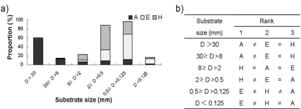
Fig. 1-7. Comparison of substrate volumes in different particle size: a) proportion (%) of substrates among different sample sites and b) nonparametric comparison of volumes between different sample sites in different substrate sizes.
Fig. 2-1. Location of the sampling sites in tributary streams of the Garonne River catchment, France. Black circles represent the different sampling sites.
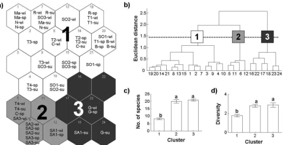
Fig. 2-2. Classification of sampling sites on the self-organizing map (SOM). a) The patterned SOM map showing the classification of sample sites according to their macroinvertebrates composition. b) Hierarchical classification of the cells of SOM map. c) Mean and SE of EPTC species richness in different clusters defined in the SOM. The Mann-Whitney test was significant for all three clusters (p<0.001). d) Comparison of the Shannon-Weaver diversity index (mean and SE) in different clusters defined with SOM (Fig. 2). The same letters indicate no significant difference.
Fig. 2-3. Distribution patterns of some species on the SOM. Scale bars indicate the weight vector of each species in corresponding SOM units.
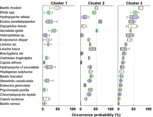
Fig. 2-4. Box plots showing occurrence probability (%) of each species in different clusters. Values were obtained from weight vectors of the trained SOM. – median, 25-75%, non-outlier range. Different colors are used simply to aid the reader in the identification of different species across the 3 clusters.
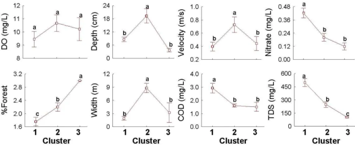
Fig. 2-5. Environmental characteristics of different clusters. Error bars indicate standard error. The same letters indicate no significant difference.
Fig. 3-1. Location of the sample sites. a) Korean Peninsula, b) the Suyong River and c) the Nakdong River.
Fig. 3-2. The map trained by SOM for pattering benthic macroinvertebrates reported from different streams in South Korea from 1984 to 2000: (a) sample sites; (b) mean and S.E. of EPT richness in different clusters defined in the SOM (n = 31 (I), n = 21 (II), n = 63 (III), n = 64 (IV)); (c) mean and S.E. of BMWP scores in different clusters defined in the SOM (n = 31 (I), n=21 (II), n = 63 (III), n = 64 (IV)). The different alphabets indicate significant difference in the Mann-Whitney test (p < 0.001).
Fig. 3-3. Profile of abundance of the prevalent taxa matched to clusters based on the trained SOM. The values in the vertical bar indicate densities (individuals/square meter).
Fig. 3-4. Monitoring of benthic macroinvertebrate communities collected at YCK in the Suyong stream from November 1992 to April 1995 according to the trained SOM (the sample was not collected in December 1994). (a) Recognition of the samples: November 1992.November 1993 (dots); January 1994.January 1995 (solid), and (b) mean and S.E. of biological and physico-chemical indices in different clusters defined in the SOM (n = 4 (I), n = 12 (III), n = 12 (IV)). The different alphabets indicate significant difference in the Mann-Whitney test (p < 0.001). Fig. 3-5. (a) Monitoring of benthic macroinvertebrate communities collected at THP in the Suyong River from March 1992 to April 1995 according to the trained SOM (n = 35). (b) Mean
and S.E. of biological and physico-chemical indices.
Fig. 3-6. Monitoring of benthic macroinvertebrate communities collected at LTER sites according to the trained SOM: (a) recognition of the samples (the number in the sample name indicates the month of collection) and (b) mean and S.E. of biological and physico-chemical indices (n = 2 (I), n = 8 (IV)).
Fig. 4-1. Relations between number of individuals in log scale and species richness in the 1970 samples used in this study. Each point indicates each sampling site. (a) All samples, (b–i) the samples separately grouped in clusters 1, 2, 3,. . ., 8, respectively.
Fig. 4-2. Log-normal model of community structure by grouping species into abundance categories (octaves, i.e. power of 2).
Fig. 4-3. Classification of the samples according to the trained SOM. (a) The SOM units were grouped to eight clusters, (b) the dendrogram according to the Ward linkage method based on Euclidean distance, (c) geographical location of the sampling sites matching to clusters according to the SOM (Fig. 3a). Cluster 6 is not indicated on the geographical map because it did not show any specific geographic area.
Fig. 4-4. Community characterization in different clusters according to the SOM (Fig. 3a). (a) Species richness (number of species), (b) abundance (different alphabets indicate significant differences between the clusters based on the Unequal N HSD multiple comparison test (p = 0.05). Error bars indicate mean and standard error of each variable).
Fig. 4-5. Environmental variables in different clusters according to the SOM (Fig. 3a). (a) Altitude, (b) depth, (c) conductivity, (d) velocity (different alphabets indicate significant differences between the clusters based on the Unequal N HSD multiple comparison test (p = 0.05). Error bars indicate mean and standard error of each variable. Conductivity was not available at the samples in cluster 1).
Fig. 4-6. Variation in biological indices in different clusters according to the SOM (Fig. 3a). (a) EPT richness, (b) EPT abundance, (c) Shannon diversity index, (d) Biological Monitoring Working Party (BMWP) score, (e) evenness (different alphabets indicate significant differences between the clusters based on the Unequal N HSD multiple comparison test (p = 0.05). Error bars indicate mean and standard error of each variable).
LIST OF TABLES
Table 1-1. Summary of environmental variables in averages (min-max) and list of abundant taxa in different clusters defined by SOM (Fig. 2).
Table 1-2. Comparison of SR and BMWP in different clusters defined by SOM (Figs. 4–6).
Table 4-1. Correlation coefficients among community parameters and biological indices used in the datasets.
Table 4-2. Community parameters, indicator species and environmental descriptions in different clusters.
GENERAL INTRODUCTION
Sustainable management of aquatic ecosystems has been one of the most urgent concerns in environmental issues due to water resource shortage and its contamination. In order to achieve successful management of aquatic ecosystems, the objective assessment of water quality is a prerequisite for execution of appropriate management polices. Such management requires the understanding of how these ecosystems function, and thus how communities are related to the environment (Lek et al. 2005). The assessments made and the predictions forecast are hoped to lead to improvements in the physical and chemical characteristics of freshwater ecosystems.
Among biological communities, benthic macroinvertebrates have been widely used for ecological assessment of water quality. Macroinvertebrates are sedentary and have intermediate life span (from months to a few years). Additionally, benthic macroinvertebrates play a key role in food web dynamics, linking producers and top carnivores. The different kinds of species had different levels of tolerance, so the community structures had higher relationship with the disturbance. It is easy to collect and identified. Consequently, macroinvertebrates have been suitable for reflecting ecological water quality (Barbour et al., 1996; Butcher et al., 2003; Davies et al., 2000; Hawkes, 1979; Hellawell, 1986; Resh et al., 1995; Reynoldson et al., 1997; Richard et al., 1997; Rosenberg and Resh, 1993; Wright et al., 1993; Wright et al., 2000).
Data for community dynamics are complex and difficult to analyze, since communities consist of many species varying in a non-linear fashion in spatial and temporal domains. There have been numerous accounts of multi-variate statistical analyses regarding characterization of community data in ecology (e.g., Bunn et al., 1986; Legendre and Legendre, 1998; Ludwig and Reynolds, 1988; Quinn et al., 1991). Data for community classification and ordination have
been available by measuring degree of association among the sampled communities and taxa (Legendre and Legendre, 1998; Ludwig and Reynolds, 1988). However, conventional multi-variate methods are generally limited in the sense that they are mainly applicable to linear data and have less flexibility in representing ecological data, for instance, handling noise and data management (Chon et al., 1996; Lek and Guégan, 1999, 2000; Recknagel, 2003).
The Self-Organizing Map (SOM) is an efficient tool for mining non-linear data and has been extensively used for patterning community data since 1990s (e.g., Chon et al., 1996, 2000, 2002; Kwak et al., 2000; Levine et al., 1996; Park et al., 2001, 2003a,b, 2004). Chon et al. (1996) classified benthic macroinvertebrate communities in polluted streams with the SOM and elucidated community patterning according to anthropogenic disturbances and locality of the sample sites.
The species richness and distribution are the main fact of the ecology research for the theoretical and conversational aims (Krebs, 1994). Along with analysis in species richness, investigation of species abundance patterns has been regarded as an important topic in elucidating patterns of communities responding to the disturbances. Preston’s canonical log-normal distribution has been the most widely accepted formalization of the relative commonness and rarity of species (Preston, 1962; Brown, 1981). Regarding that the species are often vulnerable to various environmental disturbances, the existence of rare species is a key issue in community ecology in relation to risk assessment. This type of complex relationships in ‘community changes and environment disturbances’ would be accordingly addressed by studying community compositions in relation to abundance patterns per taxa, i.e. relations between species richness and abundance.
This thesis documents bioassessment using benthic macroinvertebrates in different scale and pollution level in streams by using ecological informatics. Chapter I, we intend to reveal
changes in macroinvertebrate communities intensively collected within a limited area in a midstream reach of a polluted stream after restoration project. We investigated spatial heterogeneity by selecting the sample sites short distances (5-10m) apart, and correspondingly characterized abundance patterns of benthic macroinvertberates in different habitats. This study, in chapter II, were (i) to assess how agricultural land use disturbs EPTC assemblages at the spatial scale of reach and (ii) to employ community analyses in revealing the effect of agricultural land use. We accordingly selected reference (i.e., streamsides composed of woody and grass vegetation) and agriculture-impacted (i.e., streamsides composed of croplands) sites. Chapter III, we further elaborated to show the trained SOM as a means of providing a comprehensive view on ecological states of the communities and to use the SOM as a map for assessing biological water quality. In Chapter IV, we apply the SOM to mining the large-scale community data and to further relating the community patterns to variation caused by geographic distribution and different degrees of disturbances.
I.
Characterization
of
benthic
macroinvertebrate
communities in a restored stream by using self-organizing
map
Introduction
With the advantages of taxonomic diversity, sedentary in behaviors and long life cycles, benthic macroinvertebrates characteristically respond to anthropogenic disturbances in an integrated and continuous manner, and consequently have been widely used for assessing the water quality and ecological status of aquatic systems (Resh and Rosenberg, 1984; Hellawell, 1986; Rosenberg and Resh, 1993). There have been numerous studies on community characterization and water quality evaluation over a broad scope from clean to severely polluted states (Hellawell, 1986; Rosenberg and Resh, 1993; Barbour et al., 1996; Reynoldson et al., 1997; Richards et al., 1997; Davies et al., 2000; Wright et al., 2000; Chon et al., 2002; Butcher et al., 2003). In most cases, the surveys have been carried out in a large scale in the order of 1– 100 km between the sample sites. Species traits are usually distinct and community compositions are easy to characterize between different sites in these cases (Townsend and Hildrew, 1994; Death, 1995; Resh et al., 1994; Poff, 1997; Rabeni et al., 2002; Lamouroux et al., 2004).
Spatial heterogeneity, however, still exists in a small scale (e.g., less than one kilometer) in lotic conditions according to hydro-morphological characteristics of streams (e.g., pool, riffle, etc.) (Minshall, 1988; Poff and Ward, 1990; Townsend and Hildrew, 1994; Copper et al., 1997; Palmer et al., 1997; Palmer and Poff, 1997; Poff, 1997; Poole, 2002). Accordingly, the
community patterns are variable in different habitats in a small scale (Lancaster and Hildrew, 1993; Resh et al., 1994; Townsend and Hildrew, 1994; Armitage and Cannan, 2000; Brown, 2003; Roy et al., 2003; Gebler, 2004), although overall composition of species may not be widely variable as shown in a large scale. Benthic macroinvertebrates have been investigated in a relatively small scale of hundred-meter distances (e.g., Cummins and Lauff, 1969; Hildrew et al., 1980; Lancaster and Hildrew, 1993; Brown, 2003; Roy et al., 2003).
There have been a limited number of studies that reveal the relationships between hydraulic variables and distribution of macroinvertebrates at micro-habitats (Lancaster and Hildrew, 1993; Lamouroux et al., 2004; Brooks et al., 2005). Downes et al. (1993) described important hydro-morphological factors influencing the spatial distribution of invertebrates after investigating small scale patchness. Brooks et al. (2005) recently demonstrated the importance of small-scale differences in hydraulic conditions characterized by water velocity, depth and substrate roughness in determining the spatial distribution of macroinvertebrate assemblages in riffle habitats. The characteristics of small scale habitats are important factors for the success of stream restoration activities. Monitoring in a small scale habitat, heterogeneity provides a measure of ecosystem restoration (Pik et al., 2002). For example, Purcell et al. (2002) evaluated the effects of restoration of a small stream using benthic macroinvertebrate communities. In this study, we intend to reveal changes in macroinvertebrate communities intensively collected within a limited area in a midstream reach of a polluted stream after a restoration project. We investigated spatial heterogeneity by selecting the sample sites short distances (5–10 m) apart, and correspondingly characterized abundance patterns of benthic macroinvertebrates in different habitats.
Materials and methods
Study sites
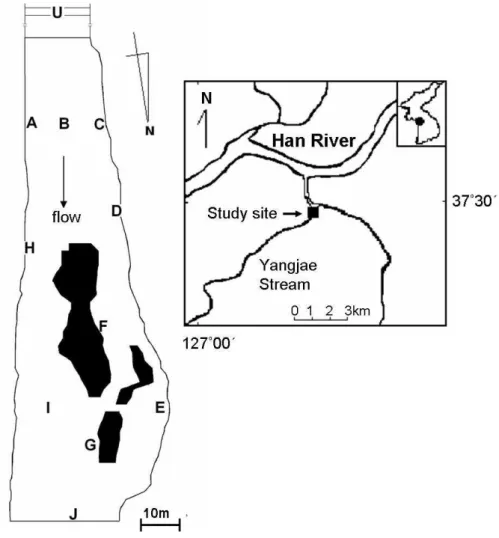
The field survey was carried out within a 200 m reach (Hakyeoul) in the Yangjae Stream, a tributary of the Han River in the south of Seoul, Korea (37°24′–37°29′N, 126°57′–127°04′E) (Fig. 1-1). It flows through the metropolitan and agricultural areas in the city, and has been mainly polluted with organic matter (KICT, 1997). The stream has a year-round flow of 20–30 m in width and 10–60 cm in depth. Water discharge rapidly increases in the period of summer flooding and decreases in the dry winter season. Recently, a campaign for water recovery has been carried out by the local government. Benthic macroinvertebrates were sampled at 11 sampling sites in the study area based on location, hydromorphological characters and a 5–10 m distance between sites (Fig. 1-1). According to topographical conditions the sample area was partitioned into three zones: 1) the upstream zone covered the sample sites located in the upper part of the sample area, and was characterized by large substrates and relatively high water velocity (sites, U, A, B, C and D), 2) the downstream zone included the sample sites with lower velocity and higher sedimentation at the lower part of the sample area (sites H, I, and J) (Fig. 1-1), and 3) the pool zone was located at the curved down stream area and were characterized with low values in water depth and velocity, and high levels of sedimentation (sites E, F, and G). Except sites U and J which were located at the upper part and the lower part of the study sites, respectively, longitudinal or curvilinear sampling was carried out to reveal local topographic characters of the sample sites.
Fig. 1-1. The sample sites located in the Yangjae Stream in the Han River, Korea.
The survey area has been partially manipulated for a restoration project of the stream. Vegetation channel revetment technique was carried out in the riparian zone close to site A (Fig. 1-1) (KICT, 1997). The stream bed was artificially planted with large-sized cobbles approximately 5 cm in diameter. The upstream islet, near where site F was located, was artificially constructed for management of siltation as well as for providing habitats for birds and other animals, while the downstream islet, around where G was sampled, was naturally formed. Restoration was also carried out on the riparian zone close to site D, but the stream bed
was not affected by the restoration project in this case. Site E was located close to the edge area at the pool zone, and silts were highly accumulated around this site.
We selected four environmental variables to reveal spatial heterogeneity in the sample area. Firstly, the water depth and velocity were used to represent hydromorphological characters of the sample sites. Secondly, considering that topographic conditions of streams affect stream beds, substrate roughness was recorded to represent spatial heterogeneity of the sample sites (Statzner et al., 1988; Poff and Ward, 1990). Lastly, the percentage of silt was measured to represent a fine level of substrate compositions, according to Statzner et al. (1988). The substrate composition in each site was measured in different diameters (D): coarse cobbles (mean D sizes≥100 mm), fine cobbles (50mm≤D<100mm), pebbles (30mm≤D<50mm), fine pebbles (16 mm≤D<30mm), coarse gravel (8 mm≤D<16mm), and the smaller substrates (4 mm≤D<8 mm, 2 mm≤D<4 mm, 1 mm≤D<2 mm, 0.5 mm≤D<1 mm, 0.25 mm≤D<0.5 mm, 0.125mm≤D<0.25mmand D<0.125mm) (Cummins and Lauff, 1969). The volumes of larger substrates (≥8 mm) were determined by the volumetric bucket in the field, while substrates smaller than 8 mm in diameter were separately sampled in plastic containers (50 ml) in triplications. Substrate roughness was expressed as K=(5C1+3C2+C3) /9, where the subscripts 1, 2 and 3 represent the 1st, 2nd and 3rdmost dominant substratum type, respectively (Statzner et al., 1988). Coarseness value C was correspondingly assigned to the size of the dominant substrates: 1, 2, 3 and 4 if the size, k, is in the range of k<0.125mm, 0.5 mm≤k<4 mm, 8 mm≤k<30 mm, k≥30 mm, respectively. The coarseness classes have been slightly modified from those given by Statzner et al. (1988) to the size used in this study.
Community data
(30 cm×30 cm, 500 µm mesh; APHA et al., 1985) approximately 10 cm in depth at monthly intervals for two years starting in April 1996. The collected macroinvertebrates were preserved in 7% Formalin solution. In the laboratory, the invertebrate specimens were sorted, identified to genus level and counted for the number of specimens under microscopes. Identification was based on Yun (1988), Brighnam et al. (1982), Merritt and Cummins (1984), Pennak (1978), and Quigley (1977). Chironomidae was separately identified based on Wiederholm (1983), while Oligochaeta was checked with Brinkhurst and Jamieson (1971) and Brinkhust (1986). In the datasets, 24 genera were identified, showing that only a few taxa were highly abundant at the polluted sample sites. Chironomidae, abundant with Chironumus sp., and Oligochaeta, mostly consisting of Limnodrilus hoffmeisteri (Tubificidae), were the dominant taxa. In order to represent water quality of the sample sites, species richness (SR) and BMWP (Biological Monitoring Working Party, Walley and Hawkes, 1997), two conventionally used biotic indices, were estimated from the sampled community data.
Modeling procedure
First we defined hydro-morphological patterns of the sample sites based on four environmental variables (depth, velocity, substrate roughness and the percentage of silt) by the learning process of SOM. Subsequently, we further revealed temporal changes in macroinvertebrate communities at the selected sites by SOM. Both environmental variables and community data were scaled between 0 and 1 in the range of the minimum and maximum values within each variable. In order to reduce high variation, abundance data used for training with SOM was log-transformed before the analysis of each taxon. SOM is an adaptive unsupervised learning algorithm and approximates the probability density function of the input data (Kohonen, 2001). SOM consists of input and output layers connected with computational
weights (connection intensities). The array of input nodes (i.e., computational units) operates as a flow-through layer for the input vectors, whereas the output layer consists of a two-dimensional network of nodes arranged in a hexagonal lattice. In the learning process of SOM, initially the input data (data matrix for either environmental variables or taxa abundance in this study) were subjected to the network. Each raw input vector consisting of the values for different environmental variables (or abundance data in different taxa) was provided sequentially as input data. In this case the number of the input node was equal to the number of variables (or number of taxa), while the output layer consisted of N output nodes (i.e., computational units) which usually constitute a 2D grid for better visualization. Subsequently, the weights of the network were trained for a given dataset. Weights were initially generated as small random numbers. Each node of the output layer computes the summed distance between weight vector and input vector. The output nodes are considered as virtual units to represent typical patterns of the input dataset assigned to their units after the learning process. Among all virtual units, the best matching unit (BMU), which has the minimum distance between weight and input vectors, becomes the winner. For the BMU and its neighborhood units, the new weight vectors are updated by the SOM learning rule. This results in training the network to classify the input vectors by the weight vectors they are closest to. The detailed algorithm of SOM for ecological applications can be found in Chon et al. (1996) and Park et al. (2003a). After training, the Ward’s linkage method based on the Euclidian distance (Ward, 1963) was applied to the weights of the nodes in SOM for further clustering (Jain and Dubes, 1988; Park et al., 2003b). After preliminary training, we used N=80 (10×8) of SOM output units for patterning samples with environmental data, and N=20 (5×4) units for patterning temporal variation of community at the selected sites. We used the functions provided in the SOM toolbox (Alhoniemi et al., 2000) in Matlab (The Mathworks, 2001).
Statistical analysis
To test the null hypotheses of no significant differences in environmental variables, taxa abundance and biotic indices in different clusters, we carried out nonparametric multiple comparisons after the Kruskall–Wallis test with the unequal number of samples (Zar, 1999), considering wide variations in community data and the different number of the samples in clusters patterned by SOM.
Results
Classification of sample sites
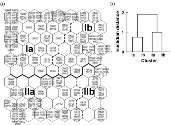
When the sample sites were trained with SOM (80=10×8 nodes) based on environmental variables, two large clusters (I and II) were formed according to the dendrogram of Ward’s linkage method (Fig. 1-2a, b). SOM output units were further subclustered into four groups (Ia, Ib, IIa, and IIb). At the highest level, SOM units were vertically divided: cluster I for the upper area and cluster II for the bottom area in the map (Fig. 1-2a). This grouping coincided with the locations of the sample sites. In cluster I, the samples were collected in both pool and downstream zones, including sites E to J (Fig. 1-1), where water velocity was relatively slower and small size substrates were more abundantly present. Additionally, some samples collected at sites C and D were grouped in cluster I. In contrast to cluster I, cluster II accommodated the sample sites (U, A, B, etc.) belonging to the upstream zone with the large size substrates where water velocity was higher.
Subclustering was further obtained based on spatial variation. Within cluster I, cluster Ia was mainly represented by the pool zone such as sites E, F and G, while cluster Ib was more
associated with the sample sites located at the downstream zone, such as H and J (Fig. 1-2a). Within cluster II, subclustering was formed based on the location of the sample sites and environmental factors. Samples located in the upstream zone were mainly grouped in cluster IIa (e.g., sample sites U, A, B, etc.), while cluster IIb accommodated various sample sites with high levels of water depth and velocity. A majority of the samples collected in summer were grouped in cluster IIb, and the flooding effect appeared more clearly at the sites belonging to the downstream zone. Environmental variables varied in different clusters of the sample sites (Table 1-1). Cluster II was characterized by a higher velocity, higher substrate roughness and lower percentage of silt, and vice versa for cluster I. Within cluster II, cluster IIa was differentiated from cluster IIb by higher levels of substrate roughness. Cluster Ia was mainly different from cluster Ib by a higher percentage of silt. Overall, environmental factors in different clusters revealed heterogeneity of the sample sites. The percentage of silt was higher at the pool zone of sites E and G, whereas lower at the upstream zone of sites U and A. Environmental variables in each cluster were made distinct by using the nonparametric Kruskall–Wallis test (Table 1-1). Differences in depth, velocity and substrate roughness were statistically significant between all clusters. The variables were generally higher in cluster II than in cluster I. Depth and velocity were in the lowest range in cluster Ia, while in the highest range in cluster IIb. Substrate roughness was lower in cluster I and higher in cluster II, showing the lowest value in cluster Ib and the highest value in cluster IIa. The percentage of silt was the same level between clusters IIa and IIb, while the percentage of silt showed the highest value in cluster Ia. The statistical results revealed differences of environmental variables in different clusters.
Fig. 1-2. Classification of the sample sites by SOM based on environmental variables measured in the Yangjae Stream in a small scale from April 1996 to March 1998: a) sample sites, and b) cluster analysis with the Ward’s linkage method. Acronyms in units stand for the samples: the letter represents the name of sample sites (see Fig. 1-1), while the numbers indicate the year and month of collection (e.g., U9604; site U collected in April 1996, A9711; site A collected in November 1997; and F9803; site F collected in March 1998).
Abundances of the selected taxa in benthic macroinvertebrates varied with different clusters (Fig. 1-3). A majority of taxa were abundant in subcluster IIa. Orthocladius sp. and Cricotopus sp., which are known to be present in recovering water (Ferringto and Crisp, 1989), were highly collected in subcluster IIa. Additionally, Tanypus sp. and other invertebrates including Erpobdella sp. and Glossiphora sp. showed the highest level of abundance in this subcluster. However, the tolerant species such as Chironomus sp. and L. hoffmeisteri showed different patterns, being most abundant in cluster Ia (Table 1-1, Fig. 1-3).
Fig. 1-3. Mean abundance of the selected taxa in different clusters corresponding to SOM (Fig. 1-2). The height of the bar represents the mean, while the whisker indicates the confidential interval (mean±0.95). The same letters located on top of the whisker indicate no significant difference (p>0.05) between clusters based on the nonparametric Kruskall–Wallis test with the unequal number of samples. Among the sampled communities, the taxa with statistical differences were only presented in the figure.
Overall, environmental variables in different clusters were associated with different patterns of taxa abundance. Cluster IIa was characterized with the highest value of substrate roughness and the lowest value of the percentage of silt (Table 1-1). Abundance of various taxa was associated with this subcluster including Chironomus sp., Orthocladius sp., Cricotopus sp., Tanypus sp., Erpobdella sp., Glossiphora sp., and Physa sp. In comparison with cluster IIa, cluster IIb was represented by the highest level of water depth and velocity due to high precipitation in summer. In this subcluster, Tanypus sp., L. hoffmeisteri and Glossiphora sp. were abundantly present.
and with the highest level of percentage of silt (Table 1-1). Subcluster Ia covered the sites E, F and G at the pool zone of the survey area (Fig. 1-2). The tolerant taxa L. hoffmeisteri and Chironomus sp. were most abundant in this subcluster. L. hoffmeisteri and Chironomus sp. belong to Tubificidae and Chironomidae, respectively, and both taxa are burrowing or tube building types, being commonly associated with soft, depositing area (Hellawell, 1986). In this subcluster, the percent of silt was at the highest level (Table 1-1). Cluster Ia was additionally associated with Cricotopus sp., Glossiphora sp. etc. In comparison with subcluster Ia, subcluster Ib was relatively higher in water depth and velocity, and was relatively lower in the amount of silt. This indicated a smaller effect of sedimentation on the sample sites (e.g., H and I) in the downstream zone. In this subcluster, the associated taxa were not as diverse as shown in cluster Ia. Orthocladius sp., Erpobdella sp. and Glossiphora sp. were each abundant in cluster Ib.
Table 1-1. Summary of environmental variables in averages (min-max) and list of abundant taxa in different clusters defined by SOM (Fig. 1-2).
The same alphabets listed in superscript of environmental variables indicate no significant difference (p > 0.05) between clusters based on the nonparametric Kruskall-Wallis test with unequal number of samples.
Temporal variation of communities
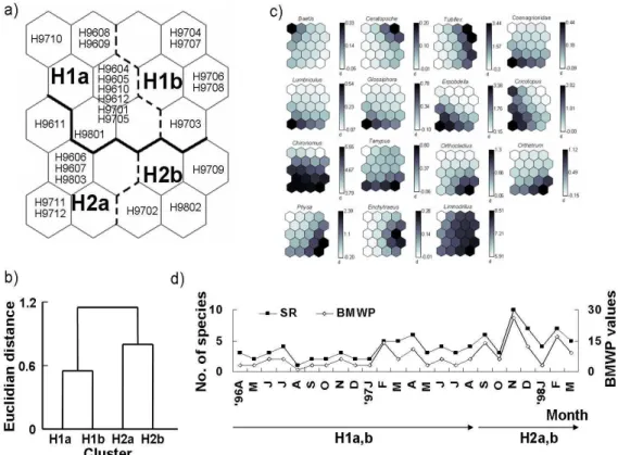
After patterning the samples based on the four environmental variables, we further chose the sample sites E, H and A, which would typically represent different clusters Ia, Ib, and IIa based on the differences of environmental factors, respectively (Fig. 1-2a), to reveal temporal variation of communities at different habitat types. The site representing cluster IIb was not chosen since the cluster was mixed with various sample sites, and a majority of the samples were observed in the temporally unstable period of summer in this subcluster (Fig. 1-2a). Community abundance data were subsequently trained with SOM (Figs. 1-4~1-6) for each site. Temporal patterns of macroinvertebrates were identified in the map. At site A representing cluster IIa, the sample sites were further divided to two main clusters with each cluster producing two more subclusters (Fig. 1-4a, b). Clusters A1 and A2 were separated according to different sampling periods. Subclusters showed further temporal changes sequentially from A1a (April 1996–January 1997), A1b (February–May 1997), A2a (June–August 1997) to A2b (September–November 1997) in the order of sampling time (Fig. 1-4a, b). In the last phase, however, the samples collected in this period belonged again to A2a (January–March 1998) after A2b (September–November 1997).
Community abundance patterns were correspondingly different in various subclusters. Different taxa appeared in a diverse manner as time progressed (Fig. 1-4c). In subcluster A1a in the earliest period, abundant taxa were not observed. The following subcluster A1b, mainly observed in March 1997, was selectively matched to Enchytraeus sp. Both tolerant genus (e.g., Chironomus sp.) and intolerant genus (e.g., Orthocladius sp., Cricotopus sp.) were also commonly grouped in this cluster. Two genera, however, were further associated with subcluster A2a in the next phase. The appearance of recovering species such as Orthocladius sp. and Cricotopus sp., indicated the recovery of water quality in the periods corresponding to
A1b–A2a (February 1997–March 1998).
Fig. 1-4. Patterning of temporal changes in macroinvertebrate communities collected at site A from April 1996 to March 1998: a) clustering of the samples in temporal variation, b) Euclidian distance between clusters, c) distribution patterns of species abundance (log-transform of (individuals/m2); indicated along with the vertical bar) in the selected taxa in different clusters. Darker color represents higher values of each variable, d) temporal variation of SR and BMWP and their corresponding clusters.
A large number of taxa were additionally present in the following subcluster A2a. Especially, Baetis, a well known genus appearing in recovering water (Hellawell, 1986), was observed in this subcluster. The appearance of Baetis sp. confirmed the phase of water recovery in the period matching to cluster A2a (Fig. 1-4c). In the following subcluster A2b, even a larger number of taxa were associated (10 genus) including various aquatic insects and other invertebrates (e.g., Erpobdella sp. and Physa sp.). L. hoffmeisteri, which was the dominant
species in the survey area, showed different patterns of occurrence compared with other species. The species was highly associated with subcluster A2b, but was also abundant over a broad area of the map (Fig. 1-4c). Biotic indices such as SR and BMWP changed accordingly with time (Fig. 1-4d). The clusters listed below x-axis (month) in Fig. 1-4d indicate the sample communities patterned by SOM (Fig. 1-4a). Subclusters appeared along with changes in biotic indices as time progressed. SR and BMWP increased gradually, peaking in October 1997 (Fig. 1-4d). The changes in indices represented the trend of water quality improvement after the restoration project. Main clusters A1 and A2 were separated according to the sampling time, June 1997. The samples grouped in cluster A1weremainly collected in the early sampling period up to May 1997, whereas the samples in cluster A2 were in the later sampling period starting from June 1997.
Fig. 5 shows temporal changes in macroinvertebrate communities collected at the sample site H, which represents the downstream zone of the sampling area defined in cluster Ib (Fig. 1-2a). Similar to site A, the samples were grouped to two main clusters according to the sampling periods (Fig. 1-5a, b). Cluster H1 mainly represented the earlier periods of the survey, whereas the samples collected at the later periods were grouped in cluster H2. Each cluster was further divided to two subclusters. However, the degree of temporal patterning at the level of subclusters was not as strong as shown in the subclustering at site A (Fig. 1-4).
Different taxa were associated with different clusters at site A (Fig. 1-5c). At the early phase in cluster H1, however, not many taxa were abundant. Subcluster H1a was loosely associated with Baetis sp., while subcluster H1b was grouped with 2 species of Ceratopsche sp. and Tubifex tubifex (Fig. 1-5c).
Fig. 1-5. Patterning of temporal changes in macroinvertebrate communities collected at site H from April 1996 to March 1998: a) clustering of the samples in temporal variation, b) Euclidian distance between clusters, c) distribution patterns of species abundance (log-transform of (individuals/m2); indicated along with the vertical bar) in the selected taxa in different clusters. Darker color represents higher values of each variable, d) temporal variation of SR and BMWP and their corresponding clusters (Fig. 1-2).
Subclusters in H2, however, were associated with diverse taxa. Both tolerant (e.g., Chironomus sp.) and intolerant (e.g., Cricotopus sp.) species were grouped in subcluster H2a. Occurrences of Cricotopus sp. along with the tolerant species, Chironomus sp., indicated recovery of water at this phase. Subcluster H2b was also diversely related to various species but were different from species composition observed in cluster H2a. Species in Chironomidae such as Orthocladius sp. and Tanypus sp. were more associated with cluster H2b. Similar to site A, the tolerant species were abundant and showed different patterns in abundance. Chironomus sp. was grouped in subclusters H2a and H2b, while L. hoffmeisteri was broadly present, covering
H1b and H2b on the map (Fig. 1-5c).
Biotic indices also varied according to different clusters at site H (Fig. 1-5d). However, the temporal patterns were not as distinct as shown at site A (Fig. 1-4d). While SR and BMWP were in the ranges of 0–15 and 0–40, respectively at site A, the indices were in narrower ranges, 0–10 and 0–30 at site H, respectively. The samples were observed in different temporal periods at the level of main clusters H1 and H2 (Fig. 1-5d). This type of grouping was revealed at the level of subclusters at site A (Fig. 1-4d). Separation of the sampling time was observed in September 1997 at site H. Fig. 6 shows temporal changes in macroinvertebrate communities collected at site E representing cluster Ia (Fig. 1-2a). Similar to the other sites, the samples were divided into two main clusters with subdivisions (Fig. 1-6a, b). Grouping patterns, however, appeared differently. Most samples were associated with cluster E1b, while only a few samples were sparsely located in other clusters. Cluster E1 was mainly sampled in the early periods of the survey, whereas cluster E2 was collected in the later periods (Fig. 1-6a). Subclustering was mostly based on differences in community abundance. Subclusters in cluster E1 were associated with the selected taxa (Fig. 1-6c). Cluster E1a was related to Tanypus (sp.) and Carabidae (sp.). Although a large number of sample sites were grouped (Fig. 1-6a), cluster E1b was associated with a limited number of taxa such as Lumbriculus (sp.) and Enchytraeus (sp.). Communities collected at the later periods in cluster E2a, however, were diverse, being grouped with Erpobdella sp., Orthocladius sp., Glossiphora sp., etc. Other taxa such as Physa (sp.), Cricotopus (sp.), and Chironomus (sp.) also appeared in cluster E2a, but they were also associated with E2b. Baetis (sp.), however, was randomly present in cluster E2b (Fig. 1-6c). Tolerant species, L. hoffmeisteri and T. tubifex showed the patterns similar to site A. They were broadly abundant over clusters E1b and E2b. Biotic indices were also variable at site E in response to temporal changes (Fig. 1-6d).
Fig. 1-6. Patterning of temporal changes in macroinvertebrate communities collected at site E from April 1996 to March 1998: a) clustering of the samples in temporal variation, b) Euclidian distance between clusters, c) distribution patterns of species abundance (log-transform of (individuals/m2); indicated along with the vertical bar) in the selected taxa in different clusters. Darker color represents higher values of each variable, d) temporal variation of SR and BMWP and their corresponding clusters.
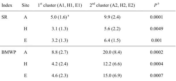
SR and BMWP showed similar patterns as those of site A (Fig. 1-4d). However, ranges of biotic indices were not as wide as at site A. The sample sites were mixed at the level of subclusters, but were differentiated by the sampling periods at the level of the main clusters. Samples in cluster E1 were collected mostly at the early sampling period up to July 1997, whereas samples in cluster E2 were present at the later sampling periods beginning in August 1997. At sites A, E, and H, both biotic indices SR and BMWP were significantly different between the early sampling periods and the later sampling periods (Table 1-2), representing
recovery of water quality at the sampling sites after the restoration project.
Table 1-2. Comparison of SR and BMWP in different clusters defined by SOM (Figs. 1-4~1-6) Index Site 1st cluster (A1, H1, E1) 2nd cluster (A2, H2, E2) P b
SR A 5.0 (1.6) a 9.9 (2.4) 0.0001 H 3.1 (1.3) 5.6 (2.2) 0.0049 E 3.2 (1.3) 6.4 (1.5) 0.001 BMWP A 8.8 (2.7) 20.0 (8.4) 0.0002 H 4.2 (2.4) 12.2 (6.6) 0.0004 E 4.6 (2.3) 15.0 (6.9) 0.0007 a
Mean (SD), b probability based on the nonparametric Kruskall-Wallis test
Discussion
The different patterns of the sample sites intensively collected in a polluted stream in the small scale were elucidated through SOM. Based on four input variables (depth, velocity, substrate roughness and silt (%)), the clusters were defined in a hierarchical manner depending on the impact of hydromorphological factors. The results confirmed the variation of the community abundance depending upon spatial heterogeneity in the small scale (Table 1-1, Fig. 1-3) (Brown, 2003; Roy et al., 2003; Brooks et al., 2005), and in biotic indices along with different time periods (Figs. 1-4d, 1-5d, 1-6d, Table 1-2). This study demonstrated that improvement of water quality could be differently monitored at the sample sites in a small scale. In general, water quality changes were more clearly addressed at site A than at sites E and H (Figs. 1-4~1-6).Communities varied depending upon the hydro-morphological condition of the
sample sites even though the locations are about 5–10 m apart. As stated above, large substrates (>30 mm) were artificially planted at site A (Fig. 1-7). At site H, which was adjacent to A, but not planted with large substrates, substrate in smaller size ranging 0.5mm–2mm were accumulated more abundantly (Fig. 1-7). Meanwhile substrate at site E was mainly composed of smaller particles less than 0.5 mm in diameter.
Fig. 1-7. Comparison of substrate volumes in different particle size: a) proportion (%) of substrates among different sample sites and b) nonparametric comparison of volumes between different sample sites in different substrate sizes.
These differences in substrates were important in characterizing the spatial heterogeneity and were therefore, crucial in determining community abundance patterns at micro-habitats. Considering that large substrates were artificially planted for the restoration project at site A, it could be stated that higher amounts of large-size substrates would accommodate diverse community composition and would reveal sensitive changes in communities, especially in the recovery of water. Consequently, large substrates used in the restoration project would be useful for monitoring community changes, confirming the previous reports that maximizing heterogeneity in ecological restoration projects may promote diverse communities and may be useful for the management of aquatic communities (Brown, 2003). There were a few samples sites unexpectedly mixed with other clusters. The sites C and D belonged to the upstream zone
(Fig. 1-1), but a majority of the samples at these sites were grouped in cluster Ia for the pool zone along with the sites E, F and G with SOM (Fig. 1-2). Hydro-morphological characters of the sites C and D, obliquely located across the sites A and B (Fig. 1-1), however, were closer to the sites in the pool zone, and were consequently characterized by slower water velocity and the increased amount of silt. Considering that biotic indices may be different according to spatial heterogeneity, consistency in selecting habitats for evaluation of biotic indices may be required. The community patterns appeared differently in each habitat (Table 1-1, Fig. 1-3), and in different temporal periods within the sample sites (Figs. 1-4~1-6). This type of sampling consistency could be further discussed in the future along with the problem of habitat suitability and patchness in spatial distribution.
Community development could be observed in regressive succession for recovery (Hawkes, 1979; Sládeèek, 1979; Hellawell, 1986) in the observed data. In recovering water, community compositions become more diverse, and these consequences were observed in community development at the sample sites in the period of water recovery (April 1996–October 1997) (Figs. 1-4d, 1-5d, 1-6d). The genus indicating recovery of water quality such as Orthocladius (sp.), Cricotopus (sp.) and Tanypus (sp.) were collected from February 1997 to March 1998. Densities of Baetis (sp.) were high from July to September 1997, while they were not collected in the corresponding periods in 1996.At the phase of higher biotic indices (July–November 1997), species in Coleoptera, Ephemeroptera and Odonata were diversely collected at low densities (Figs. 1-4c–d, 1-5c–d, 1-6c–d). The occurrence patterns of recovering species, however, were variable according to the location of the sample sites. The indicator genus such as Baetis (sp.), Orthocladius (sp.), Cricotopus (sp.) and Tanypus (sp.) were collected over a longer period at site A starting from February 1997. At site E, the indicator species were also selectively present. Certain species appeared in a longer period. Orthocladius (sp.), for instance,
was present from February to October 1997 at site E. These differences indicate that studies on community development in recovery should be also related to spatial heterogeneity. Especially in the situation of disturbance with organic pollution, spatial condition would be greatly affected by the changes in composition of substrates.
This type of study should be closely checked with the restoration process and water recovery. However, the topic on the restoration project is beyond the scope of the current study and could be further investigated in the future.
II. Agricultural land use effects on macroinvertebrates in
streams of the Garonne River catchment (SW France)
Introduction
Five interacting categories of human-induced perturbations have been reported to threaten freshwater biodiversity in a broad scope: degradation and destruction of habitats, water pollution, over-exploitation, flow modifications, and invasion of alien species (see review by Dudgeon et al., 2006). In particular, the global transition from undisturbed areas to human-dominated landscapes has strongly impacted both physical and biological features of lotic ecosystems (Allan and Flecker, 1993; Harding et al., 1998; Townsend et al., 2003; Allan, 2004). Stream ecosystems are especially vulnerable regarding spatially nested hierarchies residing in the habitats. Larger scale features (e.g., landscape, basin, segment), consequently, constrain smaller habitat units such as reaches, riffle-pool sequences and micro-habitats (Frissel et al., 1986). A great number of studies have been carried out to reveal changes in physical patterns and their influence on biological components of streams in various spatial and temporal scales, especially regarding assessment of land use impact (see review by Allan, 2004).
Agricultural land use anthropogenically modifies stream ecosystems by (i) increasing inputs of sediments, nutrients, organic matter and contaminants (i.e.; pesticides), (ii) clearing riparian vegetation and opening canopy, and (iii) altering flows and reducing habitat heterogeneity (Allan, 2004). These effects have been identified as a major cause of loss of biodiversity in agriculture-impacted catchments in streams in various studies (Lenat and Crawford, 1994; Delong and Brusven, 1998; Schulz and Liess, 1999; Hall et al., 2001; Allan,
2004).
The Garonne River basin has a long history of agricultural development (Fortuné, 1988). Forest areas were gradually replaced by agriculture lands in the Garonne River valley along with its main tributaries in the eighteenth and nineteenth centuries (see Chauvet and Descamps, 1989). Due to severe agricultural practices, the areas of the riparian forest surrounding streams were reduced to a few meters or even disappeared, while riparian forest corridors were known to enhance stream biodiversity by the flows of materials and the movement of organisms (Petersen et al., 2004; Baxter et al., 2005). Consequently, community compositions have been substantially affected by agricultural practices being carried out around the Garonne River.
Changes in community composition responding to environmental disturbances have been frequently indicated by the group of benthic insects among aquatic organisms since benthic insects have been regarded as a sensitive indicator of long-term environmental changes in water and habitat quality (Johnson et al., 1993). This group has been widely used to assess biotic integrity of streams and rivers. In particular, Ephemeroptera, Trichoptera, and Plecoptera (EPT) taxa are well documented as good biological indicators (Rosenberg and Resh, 1993). Additionally, species in Coleoptera (e.g., Elmidae), have also been reported to indicate water quality (Compin and Céréghino, 2003). Taxa richness in both groups, EPT and Coleoptera, has been used in combination to assess water quality and habitat suitability (e.g., Barbour et al., 1996; Wallace et al., 1996). We used the assemblages of both groups in elucidating the impact of agricultural disturbances in benthic macroinvertebrate communities.
Most of the studies dealing with aquatic insect assemblages of the Garonne River basin have been carried out in a larger regional scale (e.g. Céréghino et al., 2001, 2003; Compin and Céréghino, 2003). However, it is necessary to evaluate changes in communities more specifically at the local level to elucidate community-environment relationships caused by
disturbances. Small scale research has shown that spatial heterogeneity at the local level plays an important role in specifically characterizing community patterns in a polluted stream (Song et al., 2006). The aims of this study were (i) to assess how agricultural land use disturbs EPTC assemblages at the spatial scale of reach and (ii) to employ community analyses in revealing the effect of agricultural land use. We accordingly selected reference (i.e., streamsides composed of woody and grass vegetation) and agriculture-impacted (i.e., streamsides composed of croplands) sites.
Materials and Methods
Study sites
The survey area is located in the Garonne River basin in South France (between the Pyrenees and the Garonne valley near Toulouse) (Fig. 2-1), which is the third of the large French Atlantic Rivers. We investigated three tributaries of the Garonne river that mainly drain through agriculture lands: the Save stream (length (L), 143 km; catchment area (CA), 1150 km²), the Touch stream (L, 60 km; CA, 515 km²) and the Sousson stream (L, 53 km; CA, 120 km²). Four reference sites were selected in forest environment (G, T1, SA1 and R), while the other sample sites (see Fig. 2-1) were surrounded by croplands. All the sites are located between 137 and 361 m in altitude above the sea level.
Fig. 2-1. Location of the sampling sites in tributary streams of the Garonne River catchment, France. Black circles represent the different sampling sites.
Macroinvertebrate sampling
Benthic macroinvertebrates were sampled three times in each site from February to July 2004. Two samples were collected in each site. One sample was collected in the riffle zone using the Surber sampler (30 cm × 30 cm, 200 µm) while the other sampling was carried out at the sediment in the pool zone with a plastic bottle (2 cm × 10 cm × 20 cm). Samples were preserved in 70% ethanol. Ephemerotpera, Plecoptera, Trichoptera and Coleoptera (EPTC) were identified at the species level. Total EPTC richness and Shannon-Weaver diversity index were determined accordingly for the sampled communities.
Environmental variables
For each site, 8 environmental variables were measured along with the collection of benthic macroinvertebrates. Water samples were additionally collected in the riffle for measurement of Chemical Oxygen Demand (COD), Nitrate (NO3) and Total Dissolved Solid (TDS) according to the Standard Method. Dissolved Oxygen (DO) was additionally obtained using a portable meter on site. Depth, velocity and width were measured at the sampling point of benthic macroinvertebrates. The sites were also classified semi-quantitatively by the degree of riparian forest development: 1 (no riparian forest), 2 (0-10 m width of riparian forest) and 3 (forest area; > 10 m width of riparian forest).
Data analysis
SOM was utilized to cluster overall communities sampled in the survey area and to visualize environmental factors and abundance patterns of communities corresponding to the clusters. Non-linearity is generally embedded in ecological data resulting from complex interactions between environmental variables and communities (Legendre and Legendre, 1998; Lek and Guégan, 2000). The SOM (Kohonen, 1989, 2001) is an unsupervised neural network and has been implemented in various ecological researches (Chon et al., 1996;, Lek and Guégan, 2000; Park et al., 2001, 2003ab; Recknagel, 2003; Lek et al., 2005). The SOM provides an alternative to traditional ordination and classification methods (Lek and Guégan, 2000).
The SOM consists of two layers which are composed of neurons in the form of computational units: input and output layers connected with weight vectors (i.e. connection intensity). When an input vector (abundance of each species) x is sent to the input layer of the network, each neuron k of the network computes the distance between the weight vector w and the input vector x. The output layer consists of D output neurons (i.e., computational units, 24 =
6×4 in this study), which are arranged into a two dimensional grid. The best arrangement for the output layer is a hexagonal lattice, because it does not favor horizontal and vertical directions as much as the rectangular array (Kohonen, 2001). Among all D output neurons, the best matching unit (BMU), which has minimum distance between weight and input vectors, is the winner. For the BMU and its neighborhood neurons, the weight vectors w are updated by the SOM learning rule. The map size (number of output units) of the SOM is critical for accommodating hierarchical levels in community classification (Park et al., 2004). We trained the SOM with different map sizes, and chose the optimum map size based on low topographic errors (Kohonen, 2001). We looked at whether relevant groups of samples characterized distinct EPTC assemblages by performing a hierarchical cluster analysis (Ward’s linkage and Euclidean distance). To do so, we used a new matrix (24×76, output neurons x species) of the connection intensity values (i.e., vector weights) estimated by the SOM.
As a preprocessing procedure before SOM application, an abundance of 76 EPTC species were transformed with natural logarithm (i.e., log (x+1)). The transformed values were also rescaled in the range of the minimum and maximum values (i.e., 0-1) before training the model. We used the functions implemented in the SOM toolbox (Alhoniemi et al., 2000) for Matlab (The Mathworks, 2001) developed by the Laboratory of Information and Computer Science at the Helsinki University of Technology. The detailed algorithm of the SOM can be found in Kohonen (1989, 2001) for theoretical considerations, and in Chon et al. (1996) and Park et al. (2003a) for ecological applications.
Results
Characterization of EPTC assemblages
Abundance data for EPTC species provided to the SOM and the sample sites were patterned on the 2D lattice map through learning processes (Fig. 2-2a). The samples were mainly grouped according to location of the sample sites. Based on the hierarchical cluster analysis, the samples were classified into three main clusters (Fig. 2-2b). The samples from Géze (G) belonging to the reference sites were grouped in the lower-right areas of the SOM (cluster 3), while the samples (SA1-SA3) in the catchment area from the Save stream were located in the lower-left areas of the SOM (cluster 2). The samples from the other streams (e.g., Touch (T1-T4), Sousson (SO1-SO3), Marguestaud (Ma) and Rieutord (R)) were grouped widely in the upper area of the map (cluster 1). Most of the samples from the Touch and Sousson streams belonged to this group.
Community parameters could be accordingly utilized based on the SOM grouping. Species richness and Shannon-Weaver diversity indices were distinctively different among the clusters on the SOM (Fig. 2-2c). The parameters were accordingly higher in clusters 2 and 3. The Mann-Whitney test revealed that Species richness and the Shannon-Weaver diversity index were significantly lower in cluster 1 (Fig. 2-2c,d; p<0.001). This decrease in species richness and diversity suggested that the samples in cluster 1 were affected by disturbances.
Fig. 2-2. Classification of sampling sites on the self-organizing map (SOM). a) The patterned SOM map showing the classification of sample sites according to their macroinvertebrates composition. b) Hierarchical classification of the cells of SOM map. c) Mean and SE of EPTC species richness in different clusters defined in the SOM. The Mann-Whitney test was significant for all three clusters (p<0.001). d) Comparison of the Shannon-Weaver diversity index (mean and SE) in different clusters defined with SOM (Fig. 2-2). The same letters indicate no significant difference.
Figure 2-3 displays the estimated profiles of species projected on the SOM units on a grey scale. Groups of species were characteristically visualized on the SOM. Baetis vernus, Amphinemura sp. and Limnephilus spp. appeared at cluster 1. Cluster 2 was characterized by high values of Baetis fuscatus, Oligoneuriella rhenena and Heptagenia sulphurea. Hydropsyche siltalai, Brachyptera risi and Capnia bifrons appeared in cluster 3 as indicators in the reference sites. Baetis rhodani and Serratella ignita were widely distributed on the map. Caenis luctuosa and Amphinemura standfussi appeared at the right and left area on the map. The SOM clearly visualized different occurrences at the reference and polluted sites. Even the species in the same genus demonstrated contrasting tolerance to agricultural disturbances. Occurrence of Baetis vernus characteristically matched the area of cluster 1, while Baetis fuscatus mainly appeared in
the area of cluster 2 (Figs. 2-2 and 2-3). According to the SOM, Baetis vernus in the same genus could be identified as an indicator species in areas with agricultural disturbances.
Fig. 2-3. Distribution patterns of some species on the SOM. Scale bars indicate the weight vector of each species in corresponding SOM units.
Figure 2-4 shows the list of species observed in the order of abundance in cluster 3 of the reference sites. Abundance of the same taxa was correspondingly shown in clusters 2 and 3 in the figure. The gradient in the abundance pattern was accordingly observed in cluster 3 (Fig. 4, Table 1). Baetis rhodani, Elmis spp. and Hydropsyche siltalai were in the range of the highest occurrence in cluster 3, while Caenis luctuosa and Cheumatopsyche lepida were in the range of the lowest occurrence.
Abundance patterns appeared differently in clusters 1 and 2 compared with cluster 3. In cluster 1, the overall level of abundance was generally lower than the abundance shown in clusters 2 and 3. Communities in the disturbed area were characteristically collected in cluster 1.
The species abundantly collected in cluster 2 (e.g., Hydropsyche siltalai and Dupophilus brevis) were not present in cluster 1. Also, a subsequent number of species did not occur in cluster 1 (e.g., Lectura fusica, Brachyptera risi, Heptagenia sulphurea and Baetis fuscatus). Baetis rhodani was most abundant. It is notable that a wide range in abundance was observed in genus Baetis, while the level of abundance of Baetis vernus and Baetis fuscatus were in the minimum range.
The gradient shown in cluster 3 was not observed in cluster 2, although some of the abundant species (e.g., Baetis rhotani and Elmis sp.) in cluster 3 also appeared to be abundant in cluster 2. Abundance patterns in cluster 2 were found to be in the intermediate range. While the gradient shown in cluster 3 was not observed, species were more diverse compared with cluster 1. Esolus parallelepipedus, Serratella ignita and Habrophlebia sp. were more abundant, while Baetis vernus, Capnia bifrons and Psychomyiia pusilla were in the range of least abundance in cluster 2. Species occurring in low abundance in cluster 3 were mostly collected in higher abundance in cluster 2. Some selected species abundant in cluster 3 (e.g., Capnia bifrons, Habrophlebia sp. and Brachyptera risi) were collected in the lowest range in cluster 2.
Figure 2-4 provides an overall view on the patterns of occurrence in the reference and disturbed sites. Species such as Baetis rhodani and Serratella ignita were commonly observed in three clusters. Elmis spp. and Esolus parallelepipedus, however, were highly distributed in clusters 2 and 3, while they were observed to be in a low-minimal range in cluster 1. In some species, the gradients were observed across the clusters. Hydropsyche siltalai, Dupophilus brevis, and Brachyptera sp. appeared to decrease gradually from cluster 3 of the reference sites to cluster 1 of the disturbed sites. Comparison of community abundance in different clusters showed that communities in the reference sites (cluster 3) were affected by agricultural disturbances (clusters 1 and 2).
Fig. 2-4. Box plots showing occurrence probability (%) of each species in different clusters. Values were obtained from weight vectors of the trained SOM. – median, 25-75%, non-outlier range. Different colors are used simply to aid the reader in the identification of different species across the 3 clusters.
Environmental factors were accordingly different in each cluster. All of the environmental variables significantly differed among clusters (Fig. 2-5). Agricultural impact was accordingly revealed in cluster 1. Nitrate (0.01~1.11 mEq/L), COD (1.28~10.88 mg/L) and TDS (160.9~1644.7 mg/L) were in the highest range in cluster 1, while these variables were in the lowest range in cluster 3 (Nitrate; 0.04~0.19 mEq/L, COD; 0.98~2.58 mg/L, TDS; 81.5~121.4 mg/L). Similarly, the percentage of forest showed its highest level in cluster 3, in contrast to cluster 1. Depth (2~45 m), velocity (0~1.7 m/s) and width (0~12.5 m) were in the highest range in cluster 2, while DO (0.84mg/L ~12.84mg/L) was not significantly different among the clusters.