dx.doi.org/10.2140/memocs.2018.6.307
A MULTIPHYSICS STIMULUS FOR CONTINUUM MECHANICS BONE REMODELING
DANIELGEORGE, RACHELEALLENA ANDYVESRÉMOND
Bone remodelling is a complex phenomenon during which old and damage bone is removed and replaced with new one to ensure the physiological functions of the skeletal system. It involves many biological, mechanical, chemical processes at different scales. The objective of the present work is to predict the kinetics of bone density evolution by taking into account both the mechanical and the biological frameworks. In order to do so, we propose a new computational model in which the global stimulus triggering bone remodelling is the result of the contribution of a mechanical (i.e. external loads and consequent strain energy), a cellular (i.e. osteoblasts and osteoclasts activities) and a molecular (i.e. oxygen and glucose supply) stimulus. The evolution of the bone density depends on the overall behaviour of the global stimulus. More specifically, when the global stimulus is positive, bone synthesis occurs, whereas when the global stimulus is negative, resorption takes place. Although the theoretical model has been applied on a very simple two-dimensional geometry, the final results provide new insights on the influence of each stimulus on the bone remodelling process. In particular, we confirm that mechanics plays a critical role and affects the kinetics of bone reconstruction, but it highly depends on the biological events and the distribution of bone density.
1. Introduction
Bone is a continually renewed material [Frost 1987]. Trying to model its evolution has been going on for a long time since the early works of Wolff [Cowin 1986]. Every year, 5% of trabecular bone and 20% of cortical bone is renewed under applied external mechanical loads and the prediction of bone remodeling, or bone density evolution, using numerical models requires the use of appropriate theories accounting for the specific mechanophysiological phenomena occurring within the bone microstructure. Many studies have followed since; see for example [Beaupré et al. 1990; Turner 1998; Pivonka et al. 2008; Pivonka and Komarova 2010]. Re-cently, a number of models have tried to combine multiphysics and multiscales
theoretical numerical studies [Lekszycki 2002; Madeo et al. 2011; 2012; Lekszycki and dell’Isola 2012; Andreaus et al. 2014b; Giorgio et al. 2016; 2017; Scala et al. 2016; George et al. 2017b] to represent bone density evolution. Still, many diffi-culties remain in the precise understanding of the mechanotransduction processes [Lemaire et al. 2011; Sansalone et al. 2015] driving this evolution, without even accounting that in most cases, bone reconstruction also depends on initial healing stages of vascular growth together with nutrient supply [Bednarczyk and Lekszycki 2016; Lu and Lekszycki 2016].
Bone remodeling, being the result of numerous mechanobiological mechanisms, is often presented through a so-called mechanobiological stimulus, based on strain energy density, describing a variation from a state of equilibrium [Lekszycki 2002; Lekszycki and dell’Isola 2012; Scala et al. 2016]. However, for good prediction of bone remodeling, it is necessary, not only to account for the mechanical aspects, but also to account for other external sources such as biological, electrical, neuro-logical,. . . involved in the process, that can be triggered by genetic or epigenetic factors, and allowing to simultaneously control their impact on the overall response of the system as well as their interactions. For these signals, the development of a thermodynamically consistent model [Martin et al. 2017] is required together with adequate homogenization procedures [Rémond et al. 2016]. The biology also needs to be adequately quantified (for example, the kinetics of bone resorption be-ing 4 times more important than the kinetics of bone reconstruction; see [Burr and Allen 2013, pp. 85–86]) through specific multiscale theoretical models [Lemaire et al. 2006; 2010; 2015].
For example, in orthodontic bone remodeling, the applied mechanical forces on the teeth (ranging from 0.5 N to 2.5 N [Wagner et al. 2017]) lead to the alteration of the cell differentiation and activation due to oxygen percentage variation by the periodontal ligament being partially deformed. Hence, the variations in vascu-larization blood flow in the periodontal ligament and thus in the supply chain of nutrients and oxygen could be used to predict cell recruitment, proliferation and migration leading to the bone remodelling process.
In this work, a continuous theoretical numerical model is presented and used to predict bone kinetics reconstruction as a function of coupled mechanical and biological sources, of the corresponding constitutive laws, of their mutual inter-actions as well as of the kinetics of each process. The external sources used here to calculate the mechanobiological stimulus are: (i) the mechanical energy accounting for the mechanical loads sustained by the bone cells and triggering bone density evolution, (ii) the concentration of nutriments (oxygen and glucose) expressed as a function of the developed hydrostatic pressure, and (iii) the cells activity triggered by specific levels of oxygen and glucose concentration due to the applied mechanical load. The cells recruiting and migration is described via two
diffusion equations [Allena and Maini 2014; Schmitt et al. 2015; Frame et al. 2017] and the bone density variation in time is calculated by the rates of bone synthesis and resorption respectively, depending on the positiveness of the defined coupled mechanobiological stimulus [George et al. 2017a].
2. Model development
2.1. Theory. Without specific external loading conditions, the bone is in a state of mechanobiological equilibrium (under gravity) in the so-called “lazy zone” where little remodeling occurs. When external mechanical load is applied, the system is perturbed and goes out of the “lazy zone”. The modified load conditions are at the origin of the creation of a coupled mechanobiological signal that will activate bone remodelling. We define this signal [George et al. 2017a] by introducing a Lagrangian configuration BL ⊂R3[Madeo et al. 2011; 2012; Scala et al. 2016],
and a suitably regular kinematical fieldχ(X, t) that associates to any material point X ∈ BL its current position x at time t . The image of the functionχ gives at any
time t , the current shape of the body also called Eulerian configuration. We also introduce the displacement u(X, t) = χ(X, t) − X, the transformation gradient F = ∇χ(X, t), and the Green–Lagrange deformation tensor E = (FT·F − I)/2.
In the present work, only the linearized partε of E is considered.
Then the global stimulus variation1S is expressed on the Lagrangian configu-ration BL in the form
1S(X, t) =
n
Y
i =1
αiSi(X, t), (1)
where t is the time, n is the total number of external sources Si (i.e. mechanical,
biological (cellular, nutrients, . . . ), electrical, . . . ) involved in the process andαi
are their weighting coefficients, triggered by genetic or epigenetic factors, allowing to simultaneously control their impact on the overall response of the system as well as their interactions.
In this work, we consider the following external sources: Smech, which includes
the applied mechanical load through the mechanical energy developed within the system to trigger the biological actions; Smol, which coincides with glucose and
oxygen supply necessary for cell survival and work contribution; Scell, which
cor-responds to the osteoblasts and osteoclasts recruiting and migration.
(i) The mechanical stimulus Smechis expressed through the “standard” definition
of the mechanical strain energy and accounts for the applied forces and loads sus-tained by bone cells. It is defined with
αmechSmech(X, t)
=αmech Z
U(X0, t) d(X0, t) exp(−Dmech
kχ(X) − χ(X0)k) d X0, (2) with the domain of interest, αmech a weighting coefficient, Dmech the inverse of
a characteristic distance accounting for the independent effect of the source, U the strain energy density dependent on the Green–Lagrange deformation tensorε, and d being a function of the bone mass density expressed as d(X0, t) = η(ρb)/ρb,max
withη ∈ [0, 1], where ρbis the bone density andρb,maxits maximum allowed value,
being the density of compact bone (corresponding to minimum porosity). (ii) The molecular stimulus Smolis defined with
αmolSmol(X, t)
=αmol Z
(αO2cO2
+αCHOcCHO) exp(−Dmolkχ(X) − χ(X0)k) d X0, (3) with Dmol the inverse of a characteristic distance, αO2 and αCHO the weighting
coefficients for cO
2 and cCHO, the concentrations of oxygen and glucose, satisfying two partial differential equations (PDEs) as a function of the hydrostatic pressure as follows: DO2∂cO2 ∂t =0, (4) and DCHO∂cCHO ∂t =0, (5) where DO2 =DCHO=Tr(ε) + φ(εIθI⊗θI+εIIθII⊗θII), (6) with Tr the trace of a tensor, φ a scalar, εI and εII and θI and θII the principal
strains and directions and ⊗ the tensor product. In (4) and (5), it is assumed that no external sources are present, only diffusion of the concentration through the geometry is present via a heterogeneous initial distribution.
(iii) The cellular stimulus Scelldefined by the osteoblasts and osteoclasts activity
and triggered by specific levels of oxygen and glucose concentration together with the intensity of the mechanical force applied is given by
αcellScell(X, t)
=αcell Z
(αob
cob−αoccoc) exp(−Dcellkχ(X) − χ(X0)k) d X0, (7) where Dcellis the inverse of a characteristic distance,αobandαocare the weighting
respectively evolving with respect to time via two diffusion-reaction equations [Allena and Maini 2014; Schmitt et al. 2015] as
∂cob
∂t =(1 − ρb)(div Dob∇cob+βocTr(ε)coc), (8)
∂coc
∂t =(1 − ρb)[div Doc∇coc+(koc−βocTr(ε))coc], (9)
where div and ∇ are the divergence and gradient operators, the diffusion tensors Dob and Docare defined as in (6), koband kocare the osteoblasts and osteoclasts
proliferation rates, respectively with kob equal toβoc, the osteoclasts differentiation
rate. In (8) and (9), as osteoblast proliferation showed to be dependent on the applied mechanical strain [Ignatius et al. 2005; Ehrlich and Lanyon 2002], we assume on a first approximation that it is directly dependent on the volume variation the structure through the trace of epsilon. Complementarily, as the resorption of osteoclasts immediately triggers the proliferation of osteoblasts, a similar kinetic was defined for osteoclasts.
For the above PDEs (equations (4), (5), (8), (9)), a zero flux boundary condition is applied on the external free surfaces as it is supposed that there is no exchange with the outer system.
The variation of bone densityρbis described by a first order ordinary differential
equation with respect to time given by ∂ρb
∂t =Ab(ρb)[sb(1S+) + rb(1S−)], (10)
where rband sbare the rates for bone resorption and synthesis respectively,
depend-ing on the positive(1S+) and the negative (1S−) value of the global stimulus 1S. Abis a function of the bone porosity controlling the intensity of the bone
remod-eling process that needs to be defined experimentally.
Here, we consider the bone as an isotropic linear elastic material whose Young modulus Ebis given by Eb=Eb0ρb3[Currey 1988; Rho et al. 1995] where Eb0is
the initial Young modulus of the bone. The global static equilibrium of the system is expressed with the usual equation divσ + fν=0, withσ and fνthe Cauchy stress and the body forces, respectively. Finally, most of the model parameters defined in the current framework should be experimentally quantified. Some theoretical works have been carried out [Placidi et al. 2015; Misra and Poorsolhjouy 2015] trying to identify these parameters, but appropriately designed experiments should be developed in order to provide confident numerical predictions.
The proposed theoretical model was implemented using the Multiphysics Finite Element (FE) code COMSOL Multiphysics® to predict bone kinetics reconstruc-tion when applied to different mechanobiological stimuli.
Figure 1. Definition of the model geometry, boundary conditions and associated FE mesh.
2.2. Application. Following [Andreaus et al. 2014b; Giorgio et al. 2016], where the bone reconstruction kinetics was studied on a simple two-dimensional (2D) geometry, to compare the obtained results and assess the coupling between the defined variables of the model, the analytical framework described in Section 2.1 is applied similarly on a 2D cantilever beam. The beam of length L and height h is submitted to a tension F at the right side and clamped on the left side (see Figure 1).
As for the initial conditions of the problem, the left half side of the beam is filled with dense bone(ρb=0.6), whereas the right half side of the beam, where the
external load F is applied, is constituted by light bone(ρb=0.1) and is assumed to
represent a bone substitute or graft. Thus, when mechanical load is applied, migra-tion of cells and nutriments occurs from left to right with bone density increasing in both regions. The input data of the model are listed in Table 1.
These parameters were defined without a priori knowledge of the biological quantifications of the in vivo conditions and could therefore require to be tuned for a better approximation of real life conditions. Also, the global stimulus1S was artificially amplified by a multiplication factor to reduce the computation time and accelerate the bone density kinetics evolution (which is of the order of 3 months for real bone) while ensuring consistent results.
3. Results and discussion
The concentrations evolutions for osteoclasts, osteoblasts, oxygen and glucose are presented in Figure 2. From the start of the analysis, the concentrations evolve with non-linear distributions and show a clear diffusion from the left to the right of the beam leading to an increase of them on the right side of the beam.
The oxygen and glucose concentration are diffusing quicker than osteoblasts and osteoclasts as their final distribution through the length of the beam is constant at the end of the analysis (cO
2 =0.1 at cCHO =0.05), which is not the case for osteoblasts(0.08 < cob< 0.1). The osteoclasts completely disappear over time
since they differentiate into osteoblasts (initial concentration of 0.05 versus final concentration of 6 × 10⁻⁷).
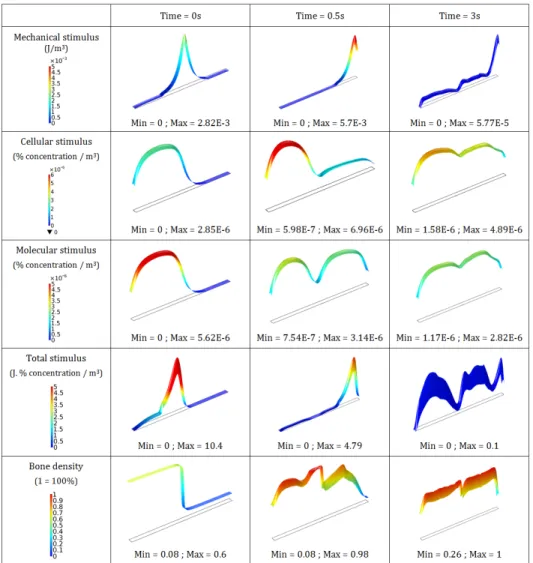
The calculated individual and global stimuli, together with bone density evolu-tion over time are presented in Figure 3.
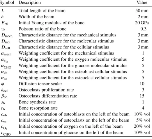
Symbol Description Value
L Total length of the beam 50 mm
h Width of the beam 2 mm
Eb0 Initial Young modulus of the bone 20 GPa
vb Poisson ratio of the bone 0.3
Dmech Characteristic distance for the mechanical stimulus 3 mm
Dmol Characteristic distance for the molecular stimulus 3 mm
Dcell Characteristic distance for the cellular stimulus 3 mm
αmech Weighting coefficient for the mechanical stimulus 1
αO2 Weighting coefficient for the oxygen molecular stimulus 5 αCHO Weighting coefficient for the glucose molecular stimulus 5 αob Weighting coefficient for the osteoblast cellular stimulus 5
αoc Weighting coefficient for the osteoclast cellular stimulus 5
φ Diffusion tensor scalar 10
kocl Osteoclasts proliferation rate 3
βob Osteoclasts differentiation rate 15
sb Bone synthesis rate 1
rb Bone resorption rate 4
cob Initial concentration of osteoblasts on the left of the beam 10% vol coc Initial concentration of osteoclasts on the left of the beam 5% vol cO
2 Initial concentration of oxygen on the left of the beam 20% vol cCHO Initial concentration of glucose on the left of the beam 10% vol
Table 1. Main parameters of the model.
The mechanical stimulus shows a peak of about 2.8 · 10−3J/m3at the beginning of the analysis which increases up to 5.7 · 10−3J/m3, propagates towards the right end side due to the external load imposed as the bone reconstruction occurs, and finally decreases to about 5.7 · 10−5J/m3 at the end of the analysis as the bone
density reaches its maximum value through the whole beam. Such distribution and kinetics are directly dependent on the kinetics of bone remodelling as the bone density increases on the right side of the beam from left to right following this peak where the maximum of the strain energy density is located. In parallel, the cellular stimulus displays a parabolic profile over the left-hand side of the beam, where cells are initially located, with a maximal value of 2.8 · 10−6at the beginning of the
analysis since a higher bone density is defined on this domain, while it is equal to 0 on the right side as no cells are present. During the analysis, cells migrate from left to right with a decrease of osteoclasts concentration and an increase of osteoblasts one. Cell stimulus increases on the left side up to a value of 6.96 · 10−6, decreases again at the end of the analysis on the left at 4.5 · 10−3, and increases continuously
Figure 2. Evolution of the osteoclasts, osteoblasts, oxygen and glucose concentration over time.
on the right up to 3.5 · 10−3 with a non-linear distribution. Correspondingly, the
molecular stimulus follows a similar trend as the cellular one but with different kinetics. The initial maximal value is 5.6 · 10−6, and it decreases over time on the
left side down to 3.14 · 10−6. Identically, it becomes more uniform over the whole
beam at the end of analysis, with minimal values at the two extremities (1 · 10−6). For the total stimulus, being the result of the multiplication effects of each stim-ulus, we still observe the peak value of the mechanical stimulus as it is much larger than the biological ones. However, it is also non-zero everywhere else due to the molecular and cellular contributions. The maximal mechanical stimulus seems
Figure 3. Time evolution of each stimulus (mechanical, cellular and molecular), the total stimulus and the bone density.
to be the main driving factor on the effect of the kinetics reconstruction on the right side of the beam. As the initial bone densities are set to 0.6 on the left side and 0.1 on the right side, at the beginning of the analysis we observe a bone density evolution on both sides being triggered by the biological contribution mainly on the left side (due to weak mechanical stimulus, but higher bone density and biological stimulus), and by the mechanical stimulus mainly on the right side (due to its high value and weak bone density with no biology contribution). Once bone density has reached a certain level (mostly reconstructed bone everywhere corresponding to an approximate value of 0.7), the influence of the mechanical stimulus decreases
since the structure undergoes a smaller strain and therefore a smaller mechanical energy is developed. Then, the biological effects become thereafter much more important and play a key role in the evolution of bone density. This impact seems to occur over longer periods of time (relative to the mechanical time kinetics) and is clearly visible on the global stimulus at the end of the analysis and on the two bone density distributions during the analysis. The mechanical stimulus moves from the mid-length to the right hand side of the beam without inhibiting the increase of the bone density on the left side where it tends towards zero. Also, the bone density is recovered on the left side due to the biological impact of the stimulus and continues to increase to reach an almost maximum density even after the mechanical effect has dropped at the end of the analysis. The above proposed model being continuous, it is assumed that cell distribution is also continuously distributed through the entire geometry, even with heterogeneous distribution. Accounting for the spatial range of cell influence requires integrating the microstructure distribution [Andreaus et al. 2014a]. This contribution needs to be integrated in future works. Finally, although the mechanical stimulus seems to play a critical role in the bone reconstruction kinetics, it also shows to be highly dependent on the biological contributions and certainly coupled with the bone density impact. In fact, high bone density leads to small strains and therefore to small mechanical stimulus for a given applied mechanical load. This has a direct impact on the cellular response within the struc-ture as higher density (lower porosity) leads to lower cell density (and distribution) and lower density (higher porosity) leads to higher cell density (and distribution) with trabecular bone structure. These effects should also be integrated since the trabecular bone kinetics requires a more specifically adapted thermodynamically consistent model as described for example in [Ganghoffer 2012; 2016; Goda et al. 2016; Louna et al. 2017], and be homogenized in order to obtain a better macro-scopic prediction. Nonetheless, the above presented mechanobiological couplings would also need to be integrated within these local frameworks in order to identify precisely the influence of the biology in the bone reconstruction kinetics.
4. Conclusion
In the present paper, a new coupled multiphysics model is proposed to compute the mechanobiological stimulus for continuum mechanics bone reconstruction, by taking into account specific mechanical (i.e. external loads) and biological (i.e. cellular migration and differentiation and nutriments supply) phenomena. The final results highlight the respective contributions of each process on the kinetics of bone density evolution. Each effect shows to have an important impact although the model parameters still require adequate quantification for better representation of specific medical applications.
References
[Allena and Maini 2014] R. Allena and P. K. Maini, “Reaction-diffusion finite element model of lateral line primordium migration to explore cell leadership”, Bull. Math. Biol. 76:12 (2014), 3028– 3050.
[Andreaus et al. 2014a] U. Andreaus, M. Colloca, and D. Iacoviello, “Optimal bone density distribu-tions: numerical analysis of the osteocyte spatial influence in bone remodeling”, Comput. Methods Programs Biomed.113:1 (2014), 80–91.
[Andreaus et al. 2014b] U. Andreaus, I. Giorgio, and T. Lekszycki, “A 2-D continuum model of a mixture of bone tissue and bio-resorbable material for simulating mass density redistribution under load slowly variable in time”, J. Appl. Math. Mech. 94:12 (2014), 978–1000.
[Beaupré et al. 1990] G. S. Beaupré, T. E. Orr, and D. R. Carter, “An approach for time-dependent bone modeling and remodeling-application: A preliminary remodeling simulation”, J. Orthop. Res. 8:5 (1990), 662–670.
[Bednarczyk and Lekszycki 2016] E. Bednarczyk and T. Lekszycki, “A novel mathematical model for growth of capillaries and nutrient supply with application to prediction of osteophyte onset”, Z. Angew. Math. Phys.67 (2016), 94.
[Burr and Allen 2013] D. B. Burr and M. R. Allen (editors), Basic and applied bone biology, Aca-demic Press, 2013. Available at https://tinyurl.com/y8j9bkmz.
[Cowin 1986] S. C. Cowin, “Wolff’s law of trabecular architecture at remodeling equilibrium”, J. Biomech. Eng.(ASME) 108:1 (1986), 83–88.
[Currey 1988] J. D. Currey, “The effect of porosity and mineral content on the Young’s modulus of elasticity of compact bone”, J. Biomech. 21:2 (1988), 131–139.
[Ehrlich and Lanyon 2002] P. J. Ehrlich and L. E. Lanyon, “Mechanical strain and bone cell function: a review”, Osteoporos. Int. 13:9 (2002), 688–700.
[Frame et al. 2017] J. Frame, P.-Y. Rohan, L. Corté, and R. Allena, “A mechano-biological model of mulit-tissue evolution in bone”, Contin. Mech. Therm. (2017), 1–31.
[Frost 1987] H. M. Frost, “Bone ‘mass’ and the ‘mechanostat’: a proposal”, Anat. Rec. 219:1 (1987), 1–9.
[Ganghoffer 2012] J.-F. Ganghoffer, “A contribution to the mechanics and thermodynamics of sur-face growth: application to bone external remodeling”, Int. J. Eng. Sci. 50:1 (2012), 166–191. [Ganghoffer et al. 2016] J.-F. Ganghoffer, R. Rahouadj, J. Boisse, and S. Forest, “Phase field
ap-proaches of bone remodelling based on TIP”, J. Non Equilib. Thermodyn. 41:1 (2016), 49–75. [George et al. 2017a] D. George, R. Allena, and Y. Rémond, “Mechanobiological stimuli for bone
remodeling: mechanical energy, cell nutriments and mobility”, Comput. Methods Biomech. Biomed. Engin.20:sup1 (2017), 91–92.
[George et al. 2017b] D. George, C. Spingarn, C. Dissaux, M. Nierenberger, R. A. Rahman, and Y. Rémond, “Examples of multiscale and multiphysics numerical modeling of biological tissues”, Biomed. Mater. Eng.28:s1 (2017), S15–S27.
[Giorgio et al. 2016] I. Giorgio, U. Andreaus, D. Scerrato, and F. dell’Isola, “A visco-poroelastic model of functional adaptation in bones reconstructed with bio-resorbable materials”, Biomech. Model. Mechanobiol.15:5 (2016), 1325–1343.
[Giorgio et al. 2017] I. Giorgio, U. Andreaus, F. dell’Isola, and T. Lekszycki, “Viscous second gradient porous materials for bones reconstructed with bio-resorbable grafts”, Extrem. Mechan. Letters13 (2017), 141–147.
[Goda et al. 2016] I. Goda, J.-F. Ganghoffer, and G. Maurice, “Combined bone internal and external remodeling based on Eshelby stress”, Int. J. Solids Struct. 94-95 (2016), 138–157.
[Ignatius et al. 2005] A. Ignatius, H. Blessing, A. Liedert, C. Schmidt, C. Neidlinger-Wilke, D. Kaspar, B. Friemert, and L. Clase, “Tissue engineering of bone: effects of mechanical strain on osteoblastic cells in type I collagen matrices”, Biomater. 26:3 (2005), 311–318.
[Lekszycki 2002] T. Lekszycki, “Modeling of bone adaptation based on an optimal response hypoth-esis”, Meccanica(Milano) 37:4-5 (2002), 343–354.
[Lekszycki and dell’Isola 2012] T. Lekszycki and F. dell’Isola, “A mixture model with evolving mass densities for describing synthesis and resorption phenomena in bones reconstructed with bio-resorbable materials”, J. Appl. Math. Mech. 92:6 (2012), 426–444.
[Lemaire et al. 2006] T. Lemaire, S. Naïli, and A. Rémond, “Multiscale analysis of the coupled effects governing the movement of interstitial fluid in cortical bone”, Biomech. Model. Mechanobiol. 5:1 (2006), 39–52.
[Lemaire et al. 2010] T. Lemaire, S. Naili, and V. Sansalone, “Multiphysical modelling of fluid transport through osteo-articular media”, An. Acad. Bras. Ciências 82:1 (2010), 127–144. [Lemaire et al. 2011] T. Lemaire, E. Capiez-Lernout, J. Kaiser, N. S., and V. Sansalone, “What is
the importance of multiphysical phenomena in bone remodelling signals expression? A multiscale perspective”, J. Mech. Behav. Biomed. Mater. 4:6 (2011), 909–920.
[Lemaire et al. 2015] T. Lemaire, J. Kaiser, S. Naili, and V. Sansalone, “Three-scale multiphysics modeling of transport phenomena within cortical bone”, Math. Probl. Eng. (2015), 398970. [Louna et al. 2017] Z. Louna, I. Goda, J.-F. Ganghoffer, and S. Benhadid, “Formulation of an
effec-tive growth response of trabecular bone based on micromechanical analyses at the trabecular level”, Arch. Appl. Mech.87:3 (2017), 457–477.
[Lu and Lekszycki 2016] Y. Lu and T. Lekszycki, “A novel coupled system of non-local integro-differential equations modelling Young’s modulus evolution, nutrients’ supply and consumption during bone fracture healing”, Z. Angew. Math. Phys. 67 (2016), 111.
[Madeo et al. 2011] A. Madeo, T. Lekszycki, and F. dell’Isola, “A continuum model for the bio-mechanical interactions between living tissue and bio-resorbable graft after bone reconstructive surgery”, Comptes Rendus Mécanique 339:10 (2011), 625–640.
[Madeo et al. 2012] A. Madeo, D. George, T. Lekszycki, M. Nierenberger, and Y. Rémond, “A second gradient continuum model accounting for some effects of micro-structure on reconstructed bone remodelling”, Comptes Rendus Mécanique 340:8 (2012), 575–589.
[Martin et al. 2017] M. Martin, T. Lemaire, G. Haïat, P. Pivonka, and V. Sansalone, “A thermody-namically consistent model of bone rotary remodeling: a 2D study”, Comput. Methods Biomech. Biomed. Engin.20:sup1 (2017), 127–128.
[Misra and Poorsolhjouy 2015] A. Misra and P. Poorsolhjouy, “Identification of higher-order elastic constants for grain assemblies based upon granular micromechanics”, Math. Mech. Comp. Syst. 3:3 (2015), 285–308.
[Pivonka and Komarova 2010] P. Pivonka and S. V. Komarova, “Mathematical modeling in bone biology: From intracellular signaling to tissue mechanics”, Bone 47:2 (2010), 181–189.
[Pivonka et al. 2008] P. Pivonka, J. Zimak, D. W. Smith, B. S. Gardiner, C. R. Dunstan, N. A. Sims, T. J. Martin, and G. R. Mundy, “Model structure and control of bone remodeling: A theoretical study”, Bone 43:2 (2008), 249–263.
[Placidi et al. 2015] L. Placidi, U. Andreaus, A. Della Corte, and T. Lekszycki, “Gedanken exper-iments for the determination of two-dimensional linear second gradient elasticity coefficients”, Z. Angew. Math. Phys.66:6 (2015), 3699–3725.
[Rémond et al. 2016] Y. Rémond, S. Ahzi, M. Baniassadi, and M. Garmestani, Applied RVE recon-struction and homogenization of heterogeneous materials, Wiley-ISTE, 2016.
[Rho et al. 1995] J. Y. Rho, M. C. Hobatho, and R. B. Ashman, “Relations of mechanical properties to density and CT numbers in human bone”, Med. Eng. Phys. 17:5 (1995), 347–355.
[Sansalone et al. 2015] V. Sansalone, D. Gagliardi, C. Descelier, G. Haïat, and S. Naili, “On the un-certainty propagation in multiscale modeling of cortical bone elasticity”, Comput. Methods Biomech. Biomed. Engin.18 (2015), 2054–2055.
[Scala et al. 2016] I. Scala, C. Spingarn, A. Rémond, Y. Madeo, and D. George, “Mechanically-driven bone remodeling simulation: Application to LIPUS treated rat calvarial defects”, Math. Mech. Solids22:10 (2016), 1976–1988.
[Schmitt et al. 2015] M. Schmitt, R. Allena, T. Schouman, S. Frasca, J. M. Collombet, X. Holy, and P. Rouch, “Diffusion model to describe osteogenesis within a porous titanium scaffold”, Comput. Methods Biomech. Biomed. Engin.19:2 (2015), 171–179.
[Turner 1998] C. H. Turner, “Three rules for bone adaptation to mechanical stimuli”, Bone 23:5 (1998), 399–407.
[Wagner et al. 2017] D. Wagner, Y. Bolender, Y. Rémond, and D. George, “Mechanical equilibrium of forces and moments applied on orthodontic brackets of a dental arch: correlation with literature data on two and three adjacent teeth”, Biomed. Mater. Eng. 28:s1 (2017), S169–S177.
DANIELGEORGE: [email protected]
ICube Laboratory, University of Strasbourg/CNRS, Strasbourg, France RACHELEALLENA: [email protected]
Institute de Biomécanique Humaine George Charpak/LBM, Arts et Métiers, ParisTech, Paris, France
YVESRÉMOND: [email protected]
ICube Laboratory, University of Strasbourg/CNRS, Strasbourg, France