A Self-Learning Solution for Torque Ripple Reduction for Non-Sinusoidal Permanent Magnet Motor Drives Based on Artificial Neural Networks

Science Arts & Métiers (SAM)

is an open access repository that collects the work of Arts et Métiers Institute of

Technology researchers and makes it freely available over the web where possible.

This is an author-deposited version published in: https://sam.ensam.eu Handle ID: .http://hdl.handle.net/10985/6821

To cite this version :

Damien FLIELLER, Ngac Ky NGUYEN, Patrick WIRA, Guy STURTZER, Djaffar OULD ABDESLAM, Jean MERCKLE - A Self-Learning Solution for Torque Ripple Reduction for Non-Sinusoidal Permanent Magnet Motor Drives Based on Artificial Neural Networks - Transaction on Industrial Electronics p.12 - 2013

Any correspondence concerning this service should be sent to the repository Administrator : archiveouverte@ensam.eu

A Self-Learning Solution for Torque Ripple

Reduction for Non-Sinusoidal Permanent Magnet

Motor Drives Based on Artificial Neural Networks

Damien Flieller, Ngac Ky Nguyen, Member, IEEE, Patrice Wira, Member, IEEE, Guy Sturtzer, Djaffar Ould

Abdeslam, Member, IEEE, and Jean Merckl´e

Abstract—This paper presents an original method, based on artificial neural networks, to reduce the torque ripple in a permanent-magnet non-sinusoidal synchronous motor. Solutions for calculating optimal currents are deduced from geometrical considerations and without a calculation step which is generally based on the Lagrange optimization. These optimal currents are obtained from two hyperplanes. The study takes into account the presence of harmonics in the back-EMF and the cogging torque. New control schemes are thus proposed to derive the optimal stator currents giving exactly the desired electromagnetic torque (or speed) and minimizing the ohmic losses. Either the torque or the speed control scheme, both integrate two neural blocks, one dedicated for optimal currents calculation and the other to ensure the generation of these currents via a voltage source inverter. Simulation and experimental results from a laboratory prototype are shown to confirm the validity of the proposed neural approach.

Index Terms—Permanent Magnet Synchronous Motor, Torque Ripple, Cogging Torque, Homopolar Current, Neuro-controller, Adaline.

NOMENCLATURE

i Stator current vector e Back-EMF vector

n Number of phases of PMSM

p Number of pole pairs

K1 Speed normalized back-EMF vector

K0 Vector containing only fundamental components of K1

K2 Vector does not containing the components of rank nq, q = 1, 2,· · · which exist in K1 θ Mechanical rotor angle

Ω Mechanical rotor speed

Ctotal(pθ) Total torque

Cem(pθ) Electromagnetic torque

Ccog(pθ) Cogging torque

Cref Desired torque

Ωref Desired speed

kopt−i Optimal function by strategy i = 0, 1, 2

iopt−i Stator current vector corresponding to strategy

i = 0, 1, 2

D. Flieller and G. Sturzer are with the GREEN Laboratory, INSA of Strasbourg, France, e-mail: [damien.flieller, guy.sturtzer]@insa-strasbourg.fr.

N. K. Nguyen is with the L2EP Laboratory, Arts et M´etiers ParisTech, Lille Cedex, France, email: NgacKy.NGUYEN@ensam.eu.

P. Wira, D. Ould Abdeslam and J. Merckl´e are with the MIPS Labora-tory, University of Haute Alsace, France, email: [patrice.wira, djaffar.ould-abdeslam, jean.merckle]@uha.fr.

I. INTRODUCTION

P

(PMSMs) are widely used in many industrial production systems due to their attractive features which are their compactness, high torque mass ratio, high efficiency and ease to be controlled. There are mainly two principal types of PMSMs which are characterized by sinusoidal or non-sinusoidal back electromotive forces (back-EMF) [1].

Whatever the PMSMs, torque ripples come from various causes [1]–[5]. The cogging torque is generated by the inter-action between the rotor magnetic field and the stator teeth even if there is no current in the stator. Another source of torque pulsation results from the interaction between the stator currents and the rotor magnetic field. Generally, this torque can be divided into two terms. The first one is due to the rotor’s magnets and the stator currents. The second one is due to the saillance. In this paper, only the first term is considered because our interest lays in the non-saillance motor. Works related to saillance motors can be found in [6]–[8].

A constant torque is highly required in many applications. Therefore, various works were proposed to minimize the undesirable torque ripple [9], [10]. These works can be divided into two categories. The techniques from the first one consists in developing the machine’s stator and rotor design to cancel the undesirable torque ripple. The magnets’s properties and how to distribute them optimally on the rotor’s surface are studied in [5], [11]–[13]. The influence of the slots/poles ratio of the machine on the torque ripple is specifically studied in [12]. The techniques from the second category are based on the stator current control. An analyze of the torque’s expression is used to calculate the best currents that cancel the torque ripple. The literature provides various techniques for the optimal current determination according to adequate transformations. For example, the individual harmonics of the Fourier’s series of the back-EMF are used in order to obtain the stator currents in [14]–[16]. The work presented in [14] optimizes the currents only for harmonics of rank 5 and 7 while the method presented in [15], [16] gives the optimal currents by calculating a pseudo-inverse matrix containing the harmonics of the back-EMF. A formula was proposed in [17] which works in the a-b-c reference frame. In this method the homopolar current is null and moreover, the loss by Joule effect is not optimal. Always in the a-b-c reference frame, the works presented in [18], [19] give the expressions of the

optimal currents. These methods are based on a Lagrange’s optimization to obtain the currents which minimize the stator ohmic losses and maintain the desired torque. While working in the d-q reference frame of Park, the authors in [20], [21] determine the expressions of the d-q optimal currents; [21] optimizes only for one harmonic of rank 6. A direct expression of the a-b-c currents is given in [22], [23] by using an extension of Park’s transformation. In [24], an adaptive process based on the Fourier series expansion is presented for a machine containing 4 pairs of poles and 24 stator slots. The flow chart proposed leads to the determination of the current

iq(pθ) in order to compensate for the 6th rank harmonic of

the torque ripple. The repetitive and iterative learning control schemes were presented in [4], [25]. Based on a vectorial approach, the generation of optimal current references for multiphase PMSM in real time is reported in [26]. This approach reduces the computing operations compared to scalar methods which generally require a large amount of calculus. The performance of the proposed method is experimentally valided in normal and fault mode (open-circuited phases). Zhao et al. in [27] recently presented an other approach based on harmonic current injection, on which the Redundant Flux-Switching Permanent-Magnet Motor (R-FSPM) can be operated with high dynamique performance and good behavior at steady-state. If the back-EMF of the R-FSPM is highly non-sunisoidal, then the current calculation with the proposed method becomes complicated.

The work presented in this paper is different from the approaches mentioned above. A torque control scheme and a speed control scheme are proposed to cancel the torque ripple, including the cogging torque. The design of the controllers are based on Adaline Neural Networks (ANNs) [28], [29]. Indeed, the learning capabilities of the ANNs allow to calculate the optimal currents which give exactly the desired torque (or a desired speed) and minimum ohmic losses. This solution can be applied for a multiphase Permanent Magnet (PM) machine under normal operation or under open-circuit fault conditions. This paper is organized as follows. The problem related to torque pulsation due to the harmonics of the back-EMF is presented in Section II. Section III presents new geo-metrical considerations leading to the optimal currents. They are based on the definition of hyperplanes whose equations depend on stator currents. Section IV proposes an original direct torque (or speed) controller based on an Adaline neural network. Simulation results in Section V and experimental results in Section VI confirm the validity of the proposed neural approach. Finally, concluding remarks are provided in Section VII.

II. PMSM’STORQUERIPPLE

The stator current and the back-EMF vectors of a n phases PMSM can be defined respectively by:

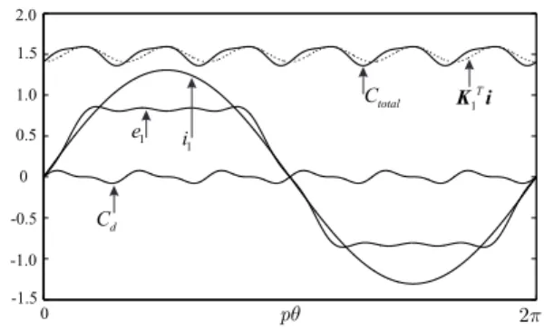
i =[ i1 i2 · · · ii . . . in ]T , (1) e =[ e1 e2 · · · ei . . . en ]T . (2) 0 -1.5 -1.0 -0.5 0 0.5 1.0 1.5 2.0 d C total C 1 T K i 1 e 1 i pq _2p

Fig. 1. Torque obtained in a non-sinusoidal three-phase machine in BLAC mode

If the machine is non-sinusoidal, we can develop the back-EMF for the ith _{phase as:}

ei= k∑max

k=1

eak,isin (kpθ) + ebk,icos (kpθ), i = 1,· · · , n,

(3) and the fundamental component of ei is:

e0i = ea1,isin (pθ) + eb1,icos (pθ), i = 1,· · · , n, (4)

where kmax is the highest considered harmonic of the

back-EMF, θ is the angular position, eak,iand ebk,i are the Fourier

coefficients. p is the number of pole pairs.

The speed normalized back-EMF vector K1 can be ex-pressed by: K1= 1 Ω [ e1 e2 · · · ei · · · en ]T . (5)

We can define K0 by: K0= 1 Ω [ e0 1 e02 · · · e0i · · · e0n ]T , (6)

where Ω = dθ_dt is the rotor’s speed.

The total torque of the machine is given by:

Ctotal(pθ) = Cem(pθ) + Ccog(pθ), (7)

with Cem(pθ) = KT1i which represents the electromagnetic torque of the interaction between the stator currents and the rotor’s magnetic field. Fig. 1 shows the current and the back-EMF of phase 1 as well as the total torque of a non-sinusoidal three-phase machine. It is obvious that the sinusoidal excita-tion currents reveal a torque pulsaexcita-tion. To supply the machine correctly, we have to determine the stator current for each phase such that the desired torque Cref is obtained.

Ccogis the cogging torque which can be expressed by [11],

[30], [31]:

Ccog(pθ) = lmax

∑

l=1

Ccoga,mlsin (mlpθ) + Ccogb,mlcos (mlpθ)

= lmax ∑ l=1 Ccog,mlcos (mlpθ + φml) , l = 1, 2, 3 . . . (8)

TABLE I

RELATIVE ANGULAR FREQUENCIES OF THE COGGING TORQUE PULSATIONS IN A THREE-PHASEPMSM (n = 3) [30], [32]

Winding Ns 2p angular frequencies mlp of Ccog

Distributed 18 6 18, 36, 54,. . .

36 6 36, 72, 108. . .

9 6 18, 36, 54,. . .

Concentrated 12 10 60, 120, 180. . .

12 14 84, 168, 252,. . .

where mp is the least common multiple of the number of stator slots Ns and the number of poles. We have:

Ccog,ml= √ C2 coga,ml+ Ccogb,ml2 , (9) tan φml=− Ccoga,ml Ccogb,ml . (10)

Tab. I gives the angular frequencies of the pulsation of the cogging torque in a three-phase machine (n = 3) for several feasible combinations of slot number and pole number of PMSM [30], [32].

Our goal is to cancel the torque ripple and we’ll obtain:

Ctotal(pθ) = Cref. (11)

From now, a torque analysis is necessary to design an efficient controller. Indeed, we want to establish a relation-ship between the back-EMF and the torque. This allows to determine the coefficients of the current harmonic terms and therefore allows to eliminate several or all undesirable torque harmonic terms. In steady state, when the stator current is:

ii= h∑max

h=1

iah,isin (hpθ) + ibh,icos (hpθ), i = 1,· · · , n,

(12) the electromagnetic torque is then given by:

Cem(pθ) = C0+

q∑max

q=1

Ca,qn′sin (qn′pθ) + Cb,qn′cos (qn′pθ),

(13) where n′ = 2n if the back-EMF contains only odd or even harmonic components,hmax and qmaxn′ are the highest

harmonics of stator currents and electromagnetic torque re-spectively. In the general case, when the back-EMF contains both odd and even harmonic terms, we have n′ = n. This analyze is obtained by an extension of the work presented in [15]. C0is the mean value and Ca,qn′, Cb,qn′are the Fourier

coefficients of Cem(pθ). qmax is determined by:

qmax= integer( kmax+ hmax n′ ). (14) We note: Cqn′= √ C2 a,qn′+ C 2 b,qn′. (15)

The compensation of the torque ripple leads to:

C0= Cref (16)

and this condition is obtained when:

q∑max

q=1

Ca,qn′sin (qn′pθ) + Cb,qn′cos (qn′pθ) =−Ccog(pθ).

(17)

TABLE II

RELATIVE ANGULAR FREQUENCY OF THE TORQUE PULSATIONS IN A THREE-PHASEPMSM (n = 3) [31] h k 1 3 5 7 9 11 13 15 17 1 0 6 6 12 12 18 3 0,6 6,12 12,18 5 6 0 12 6 18 7 6 12 0 24 9 6,12 0,18 6,24 11 12 6 18 0 24 6 13 12 18 6 24 0 30 15 12,18 24 0,30 17 18 12 24 6 30 0 19 18 24 12 30 6 36 21 18,24 12,30 6,36

The torque pulsations produced by the stator current com-ponents h and the back-EMF comcom-ponents k for a three-phase machine are given by Tab. II [31]. It is obvious that a non-sinusoidal PMSM exited by non-sinusoidal currents gives a torque pulsation. In order to supply the machine correctly, the stator current for each phase must be determined so that:

KT₁i = Cref− Ccog(pθ). (18)

There is an infinity of solutions i for (18) and we aim to obtain one giving a minimum ohmic losses. In [19], [20], [33], [34], solutions are obtained from an optimization based on Lagrange’s method to derive the stator currents. The work presented thereafter will complete these solutions by using a geometrical approach to deduce the optimal currents. Furthermore, the optimal currents can be easily obtained by a feed-back current control scheme based on an Adaline neural network. It should be noticed that these currents give exactly the desired torque by taking into account the cogging torque.

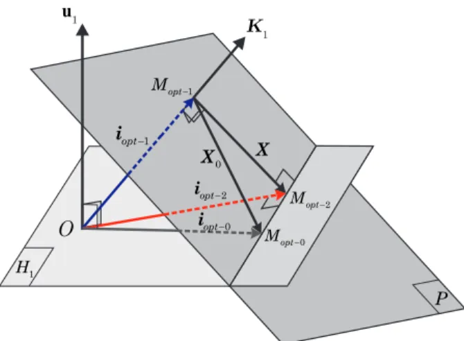
III. GEOMETRICAL INTERPRETATION OF THE THREE OPTIMAL CURRENTS

(18) is an equation of a hyperplane. Let P be the hyperplane that contains all points M whose coordinates are equal to i and which satisfies (18). K1 is thus normal to P .

In the case of a star coupled machine, the zero homopolar current constraint can be introduced by:

uT₁i = 0, (19) with u1= [ 1 1 · · · 1 ]T,∥u1∥ 2 = n.

(18) is also an equation of an other hyperplane. Let H1be a second hyperplane where all points M verify (19). u1 is thus normal to H1. P and H1 are represented on Fig. 2.

First, we try to find i = iopt−0 proportional to K0: iopt₋₀= kopt₋₀K0. (20) From (18) and (20), we have:

kopt−0=

Cref − Ccog(pθ)

KT1K0

, (21)

and finally, we obtain: iopt₋₀= Cref − Ccog(pθ) KT₀K1 K0= Cref− Ccog(pθ) KT₁K0 K0. (22)

1 u 1 K 1 opt M -1 opt -i X 2 opt -i 2 opt M -1 H O P -0 opt M -0 opt i 0 X

Fig. 2. Geometrical representation of the three optimal current vectors

iopt−0, iopt−1, iopt−2

1 u 1 K

O

Fig. 3. Geometrical representation of the three vectors K0, K1, and K2

The current of the ith _{phase is therefore:} iopt−0,i= Cref− Ccog(pθ) n ∑ k=1 eke0_k Ωe0_i. (23)

It should be noticed that iopt−0always gives a zero homopolar

current. This solution is represented by the point Mopt₋₀

on Fig. 2. iopt₋₀ does not give the minimal ohmic losses.

Let us define Mopt₋₁, represented on Fig. 2, that belongs to

the hyperplane P and is nearest point to the origin O. We will show that taking some geometrical considerations allows to easily derive the expression of the current vector iopt−1,

corresponding to Mopt−1, which has the minimal module. The

current iopt−1 is thus proportional to K1, so: iopt−1= ( KT1 ∥K1∥ iopt−1 ) K1 ∥K1∥ , (24) with K1

∥K1∥ is the unit vector in the direction of K1. From (18),

we have KT

1iopt−1= KT1iopt−0, and (24) becomes:

iopt−1= ( KT₁ ∥K1∥ iopt−0 ) K1 ∥K1∥ , (25) and with KT₁K1=∥K1∥ 2 , we obtain: iopt₋₁= (Cref − Ccog(pθ))

KT₁K0 KT₁K0 K1 ∥K1∥ 2 =Cref− Ccog(pθ) KT₁K1 K1. (26)

iopt₋₁ gives the minimal ohmic losses and the ith phase can

be written as follow: iopt_−1,i= Cref − Ccog(pθ) n ∑ k=1 ek2 Ωei. (27)

In a star connected machine, we have to introduce the additional constraint given by (19).

Let us define Mopt₋₂, represented on Fig. 2, that belongs

to the intersection of H1 and P and is nearest to the origin O. Once again, we will show that taking some geometrical

considerations allows to easily derive the expression of the current vector iopt₋₂, corresponding to Mopt₋₂, which has the

minimal module.

The current iopt−2 is proportional to K2: iopt−2= ( KT₂ ∥K2∥ iopt−2 ) K2 ∥K2∥ , (28)

where K2 is determined by (Fig. 3): K2= K1− KT1u1 ∥u1∥2 u1= K1− uT1K1 u1 n. (29)

It can be seen from (29) that K2 does not contain harmonics components of rank nq, q = 1, 2,· · · which exist in the vector K1. K2 can thus be expressed by:

K2= 1 Ω [ e′₁ e′₂ · · · e′_i · · · e′_n ]T, (30) where: e′_i=ei− 1 n k∑max k=1 ek = k_∑′_max k=1,k̸=nq

eak,isin (kpθ) + ebk,icos (kpθ), i = 1, . . . , n.

(31)

k′_maxis the highest component of e′_i and k_max′ = kmaxwhen

kmax̸= nq. From (18), we have: KT₁iopt₋₂= KT1iopt₋₀ (32) where: KT₁iopt₋₂= ( K2+ KT₁u1 ∥u1∥ 2u1 )T iopt₋₂ = KT2iopt₋₂ (33) KT1iopt−0= ( K2+ KT1u1 ∥u1∥ 2u1 )T iopt−0 = KT2iopt−0 (34)

We can thus deduce:

From (22) and (35), the expression (28) becomes: iopt−2= ( KT₂ ∥K2∥ iopt−0 ) K2 ∥K2∥ = ( KT2K0 KT2K2 Cref − Ccog(pθ) KT1K0 ) K2. (36) From (29), we obtain: KT2K0= KT1K0. (37) Moreover, from the Pythagorean theorem:

KT2K2= KT1K1− ( KT₁u1 )2 ∥u1∥ 2 = K T 1K2= KT2K1. (38) According to (37) and (38), we obtain the expression of iopt₋₂

as follow:

iopt−2=

Cref− Ccog(pθ)

KT1K2

K2. (39)

The expression for the ith phase current (iopt−2) is given by:

iopt_−2,i= Cref − Ccog(pθ) n ∑ k=1 ( ek−n1 n ∑ l=1 el )2 ( ei− 1 n n ∑ l=1 el ) Ω = Cref − Ccog(pθ) n n ∑ k=1 ek2− (_∑n k=1 ek )2 ( nei− n ∑ l=1 el ) Ω. (40)

iopt−2is the current vector which offers less ohmic losses with

zero homopolar current.

This section has developed the expressions of optimal currents which are already presented in various works by using different approaches. Indeed, iopt−0 is identical to the

solution given in [17]. Based on the Lagrange’s optimization, the currents iopt₋₁ and iopt₋₂ are also obtained in [19],

[20], [35]. Our solution leads to the same results. We give a completed geometrical representation on which we can easily determine these different optimal currents.

Expressions (22) (26) and (39) can be generalized to faulty conditions. In the faulty phases, the current can be null (open circuit), equal to a saturation value, or be a short-circuit current. The current of the healthy phases can be calculated if the defect conditions are known by imposing the desired torque, minimizing Joule losses, and fulfilling the constraints on the homopolar current (free or null). But, it is difficult to determine in real time the cogging torque and the nature of the fault. A learning schemes based on an Adaline network is thus proposed as a torque controller to provide the Fourier’s coefficients of an optimal function. This technique will thus be able to calculate the desired optimal currents on real time. This main contribution is presented in the following section.

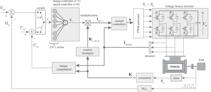
IV. TORQUE AND SPEED CONTROLLERS BASED ON

ADALINE NEURAL NETWORKS

A. Principal ideas for the torque and speed control

The optimal current is a product between kopt−i(pθ) with

the vector Ki, i = 0, 1, 2. The optimal currents iopt−i can be

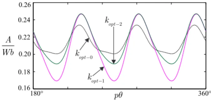
0.16 0.18 0.20 0.22 0.24 0.26 180° _pq 360° 0 opt k -2 opt k -1 opt k -A Wb

Fig. 4. Three optimal functions kopt−iin a non-sinusoidal back-EMF vectors

kopt-1 y 1 N=1 y₁N=2,3,4,5,6» 270° _pq 360° 0.16 0.18 0.20 0.22 0.24 0.26 A Wb

Fig. 5. Optimal function kopt−1 obtained for different values of N

(mlmax= 12, qmaxn′= 12, qmaxn′= 18 is negligible)

rewritten as: iopt₋₀= Cref − Ccog(pθ) KT₁K0 K0= kopt₋₀(pθ) K0, (41) iopt₋₁= Cref− Ccog(pθ) KT 1K1 K1= kopt₋₁(pθ) K1, (42) iopt₋₂= Cref− Ccog(pθ) KT 1K2 K2= kopt₋₂(pθ) K2. (43) Fig. 4 gives the shapes of the three optimal functions kopt_−i

corresponding to a cogging torque and to a non-sinusoidal back-EMF (the Fourier’s components of the back-EMF are given in section V-A).

The optimal functions kopt_−i(pθ) with i = 0, 1, 2 can be

written by a sum of Fourier’s terms as follow:

kopt−i= k0−i+

N

∑

q=1

(kaqn′−isin(qn′pθ) + kbqn′−icos(qn′pθ)) .

(44) The functions kopt−i(i = 0, 1, 2) will be learned and

synthe-sized by an Adaline network.

The value of N is important in order to compensate for the torque ripple and has to be determined correctly. This value can be obtained after a mathematical decomposition of the optimal function kopt−i. We present the development of

kopt−1. Based on the value of N for kopt−1, we can determine

the ones for kopt−0 and kopt−2. Indeed, the product of KT1K1 can be expressed as:

KT₁K1= A0+

q∑max

q=1

Aqn′cos(qn′pθ + ψqn′) (45)

where qmax= int (2kmax

n′

) .

ref

C

Voltage Source Inverter

+ torque computation em C timer m q motor i K i y torque controller speed controller load control strategies 1 S 3 S 5 S dc V 2 S S₄ S₆ M PMSM PWM generator 1 6 S -S PLL ref W å + m W s=0 s=1 switch estimation 0,1,2 i= K current controllers opt i -i measure multiplication S å (s=1) (s=0) 2 +1 termsN e

Fig. 6. Torque or speed control scheme for a PMSM based on an Adaline neural network

When the coefficients Aqn′ << A0, we can write: 1 KT 1K1 ≈ 1 A0 ( 1− q∑max q=1 Aqn′ A0 cos(qn′pθ + ψqn′) ) . (46) Finally, we obtain: kopt−1= Cref − Ccog(pθ) KT 1K1 =C0 A0 ( 1− lmax ∑ l=1 Ccog,ml C0 cos(mlpθ + φml) − q∑max q=1 Aqn′ A0 cos(qn′pθ + ψqn′) ) . (47)

By observing (47), we notice that the Adaline can estimate correctly the function kopt−1if the input vector x contains all

the terms presented in kopt−1. So, the highest rank of Adaline’s

input (N n′) has to be:

N n′ = max ( mlmax, int ( 2kmax n′ ) n′ ) . (48) With the same development, we determine N for the kopt−0:

N n′= max ( mlmax, int ( kmax+ 1 n′ ) n′ ) , (49) and for the kopt₋₂:

N n′= max ( mlmax, int ( kmax+ kmax′ n′ ) n′ ) . (50) Fig. 5 shows the estimation of kopt−1 with different values

of N (the machine’s parameters are given in section V). We can see that a good estimation is obtained when N ≥ 2.

For the three strategies, the vector containing the Fourier coefficients must be determined:

w∗i =

[

k0−i kan′−i kbn′−i .. kaN n′−i kbN n′−i

]T

.

(51)

Based on this, a torque control and a speed control can be synthesized in one single scheme represented by Fig. 6. The switch s allows to chose between the torque control or the speed control (s = 1 or s = 0 respectively) according to the inverter’s characteristics and to the machine’s coupling. The functions kopt−i (i = 0, 1, 2) will be learned and synthesized

by the Adaline network of the controller based on the three possible strategies:

• Strategy 0: Only the fundamental component of the back-EMF is used. This strategy can be used for all machines and all couplings with or without a neutral line.

• Strategy 1: The back-EMF is used completely, with all its harmonic components. This strategy can be used for star-coupled machines without a neutral line, which does not have harmonic components that are multiple of three in their back-EMFs, or all the machines that support a homopolar current.

• Strategy 2: The back-EMF is used without its harmonic component of rank multiple of n. This strategy can be used for all star-coupled machines without a neutral line. The Adaline controller takes the place of the traditional torque or speed controller for ensuring the convergence of the motor’s torque or speed toward the desired ones. All the torque ripples are compensated. The details about the Adaline are presented in the next section (Ki can be obtained off-line by another

Adaline, see Section VI-A).

B. Adaline-based controller design

Adaline’s structure is shown in 7. The rule of the torque or the speed controller based on the Adaline is to provide the optimal functions kopt−iwith i = 0, 1, 2. The same input

vector of the Adaline is used for the three strategies : x =[ x0 sin(n′pθ) cos(n′pθ) · · ·

sin(N n′pθ) cos(N n′pθ) ]T (52)

where θ is supposed to be close to θmwhich is measured by

0k w -an i w ¢-sin m n pq¢ sin m Nn pq¢ cos m Nn pq¢ M å 0k w -1 w0i w -0 x M LMS

x

e

y

+

Fig. 7. Adaline-based torque or speed control

For each control strategy, the weights of Adaline are defined by:

wi=

[

w0−i wan′−i wbn′−i .. waN n′−i wbN n′−i

]T

.

(53) The output of Adaline is then:

yi= wiTx

=w0−ix0+

N

∑

q=1

(waqn′−isin(qn′pθ) + wbqn′−icos(qn′pθ)) .

(54) The Adaline weights are solved using an iterative linear Least Mean Squares (LMS) algorithm [36] in order to minimize the torque or speed error. The weights of the Adaline can be inter-preted, giving thus a non negligible advantage to the Adaline over other types of ANNs. The Adaline is well-suited and ideal for approximating and learning linear relations. It will thus be used to learn the expressions previously developed. The Adaline weights are adjusted at each sampled time k:

wi(k + 1) = wi(k) + ηϵx xT_x = wi(k) + ηϵx x2 0+ N , (55) where η is a learning rate [36], ϵ is the torque or speed error. On each iteration, the weights of Adaline are enforced to converge toward the amplitudes of current corresponding to the control strategy. After convergence,

wi(k)−−−→_k→∞w∗i, (56)

where w∗_i is the optimal solution given by (51). Finally, the output of Adaline yi converges toward kopt_−i.

V. SIMULATION RESULTS

In this section, simulation results are presented to evaluate and to compare the performances of the approaches previously developed. A non-sinusoidal three-phase PMSM (n = 3) is considered and a constant torque of 1.5 N.m is desired.

-0.5 0 0.5 -10 -5 0 5 10 0.05 0.10 0.15 0.20 0.25 0.30 a) b) c) d) 1 e W 0 opt k _- kopt-1 kopt-2 0 opt i -1 opt i -total C 2 opt i -cog C -0.5 0 0.5 1.0 1.5 2.0 0 _(rad) 3 e W 2 e W 8 10 6 4 2 pq

Fig. 8. Simulation results of a three-phase non-sinusoidal machine: a) Φ′1, Φ′2, Φ′3 (Wb); b) kopt−0, kopt−1 and kopt−2 (A/Wb) obtained by the Adaline controller; c) optimal currents (one phase) obtained with three approaches (A); d) torque developed (N.m)

A. Case without a cogging torque

The following numerical example is taken. The non-sinusoidal three-phase PMSM has no cogging torque and a speed normalized back-EMF for the first phase expressed by:

e1(pθ)

Ω =pϕf 1sin(pθ) + 3pϕf 3sin(3pθ) + 5pϕf 5sin(5pθ) +7pϕf 7sin(7pθ) + 9pϕf 9sin(9pθ) (57)

with ϕf 1 = 0.1223 Wb, ϕf 3 = 0.0258 Wb, ϕf 5 = 0.0027

Wb, ϕf 7 = −0.0049 Wb, and ϕf 9 = −0.0054 Wb. In this

case, kmax = 9 (according to (3)) and kmax′ = 7 according

to (31). e1 contains only odd terms, the ranks of torque ripple is thus 2qn = 6q and q = 1, 2, 3.

According to (49), (48), (50), we chose 6N = 18 to reach an optimal solution. Fig. 8 shows the performances of the neural torque control with 6N = 18. More precisely, Fig. 8 a) shows the flux linkage, Fig. 8 b) shows the three optimal functions

0.98 1.00 1.02 1.04 1.06 2 0 opt -i 2 1 opt -i 2 2 opt -i 5.2% _4.9% 0 1 2 control strategies ohmic losses (pu)

Fig. 9. Ohmic losses (in pu) given by the three torque control strategies

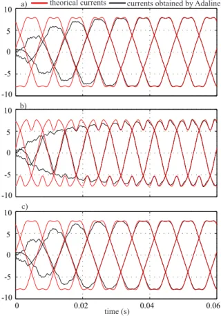
0 0.02 0.04 0.06 -10 -5 0 5 10 a) b) c)

theorical currents currents obtained by Adaline

time (s) -10 -5 0 5 10 -10 -5 0 5 10

Fig. 10. a) iopt−0 obtained with (41) learned by an Adaline ; b) iopt−1

obtained with (42) learned by an Adaline; c) iopt−2obtained with (43) learned by an Adaline (Ω = 314rad/s and η = 0.1)

Fig. 8 c) gives the shapes of the three optimal currents obtained with three strategies and Fig. 8 d) shows the total torque developed. It can be seen that the approach based on iopt₋₀

gives the same results than the one based on iopt−2 since these

two currents are close.

The stator’s ohmic losses have been estimated for the three approaches. Fig. 9 confirms that the ohmic losses ob-tained with iopt−1 are minimum. The currents iopt−0 present

5.2 % more ohmic losses and the losses of iopt−2 are lightly

smaller. iopt−2 are thus the optimal solution for a machine

which does not have a homopolar current. Fig. 10 shows the currents iopt−0, iopt−1 and iopt−2 obtained by learning

1.44 1.46 1.48 1.5 1.52 1.54 1.56 6N 6 total C = 6N 12 total C = 3.3% total C D = 0 (rad) 1 2 3 4 5 6 pq

Fig. 11. Torques Ctotal(N.m) obtained when 6N = 6 and 6N = 12 with

strategy iopt−2 0 0.15 0.20 0.25 -10 -5 0 5 10 -0.5 0 0.5 1.0 1.5 2.0 0.30 1 opt k - kopt-2 0 opt k -2 cog C Ctotal (rad) a) b) c) 10 8 6 4 2 pq 0 opt -i i_{opt -}1 i_{opt -}2 1 with opt -i 0 with opt -i 2 with opt -i

Fig. 12. Control performance with a cogging torque; a) kopt−0, kopt−1

and kopt−2(A/Wb) obtained by the Adaline controller; b) optimal currents obtained with three approaches (A); c) torque developed (N.m) and cogging torque (N.m)

respectively (41), (42) and (43) with an Adaline. We can see that the convergence of all strategies is obtained approximately in one round.

B. Case with a cogging torque

To clarify the performance of the proposed control strategy, a cogging torque is now introduced under the same previous conditions. Let us thus consider the following cogging torque:

0 0.2 0.4 0.6 -20 -10 0 10 20 -0.5 0 0.5 1.0 1.5 2.0 0 (rad) 1 with opt -i 0 with opt -i 2 with opt -i total C 2 cog C 1 opt k - opt 2 k -0 opt k -a) b) c) with PI controller 10 8 6 4 2 pq 0 opt -i i_{opt -}1 i_{opt -}2

Fig. 13. Control performance with a cogging torque and a fault on one phase; a) kopt−0, kopt−1and kopt−2(A/Wb) obtained by the Adaline controller; b) optimal currents obtained with three approaches (A); c) torque developed (N.m) and cogging torque (N.m)

The simulated results with a cogging torque are shown by Fig. 11 which compares the total torques obtained for the strategy based on iopt₋₂ with two cases, i.e., 6N = 6 and

6N = 12. This figure shows that for 6N = 6, the torque of rank 6 is completely compensated but the torques of ranks 12, 18 and 24 are only partially eliminated. Finally, the torque ripple results in ∆Ctotal= 3.3 %. In the second case, it can

be seen from the same figure that the torque ripples of rank 6, 12 and 18 are perfectly eliminated for 6N = 12. For this value of N = 2, Fig. 12 shows the optimal functions and the optimal currents, kopt−i and iopt−2 with i = 0, 1, 2, and

the resulting torques. It can be seen that all torque ripple, including the cogging torque, is elimined. Finally, we have

Ctotal= Cref = 1.5 N.m.

C. Case with a cogging torque and a fault on one phase

Simulations with a faulty machine are performed to confirm the validity of the proposed method. An additional pulsation of the electromagnetic torque always appears when one of the machine’s phases is faulty. The compensation of this pulsation is ensured by the healthy phases. In the following, the third phase of machine is faulty and the results are presented by Fig. 13. In spite of a faulty phase, the control based on the three strategies are able to maintain the torque as a constant. Comparatively to the results obtained in Fig. 12 (with a

Dspace 1104 current sensor inverter incremental encoder PMSM & load PC transformer Fig. 14. Experimental platform setup

cogging torque but no faulty phase), it can be seen that there are more harmonics in the optimal functions kopt−i in the

presence of a fault. According to the training capabilities of the Adaline, these harmonics are adjusted in real time in order to produce the currents that compensate for the torque pulsation created by the faulty phase. Finally, a desired constant torque is obtained.

The proposed neural approaches are also compared to a PI (Proportional Integrator) controller under the same faulty conditions. Fig. 13 c) shows the irregular behavior of the torque obtained by the PI controller. The neuronal controller based on the optimal strategies is more efficient. Maintaining a constant torque under faulty phase conditions remains a difficult task.

VI. EXPERIMENTAL RESULTS

A three-phase non-sinusoidal machine PMSM with Rs= 3

Ω, Ls= 12.25 mH and a pair poles number p = 3 is connected

to a three-phase Voltage Source Inverter (VSI). The rotor’s position as well as the stator currents are measured in real-time by using an incremental coder and currents sensors. The measures are sent to a process running on a dSPACE DS1104 board hosted by a PC. The process consists of the control algorithm based on the proposed strategies which provides the signals sent to a PWM generator for the control the inverter.

A. Speed normalized back-EMF estimation

In practice, the PMSM is actuated by an induction machine which has no cogging torque in order to precisely estimate the speed normalized back-EMF. In this experiment, the speed and the back-EMF are measured by standard sensors. The speed normalized back-EMF depends on the internal structure (rotor and stator) of the machine and its amplitude is not related to the rotor speed.

The optimal functions are learned with an Adaline network with an input vector composed of cos kpθ and sin kpθ terms with k varies from 0 to 15. After convergence, the signal k1=

0 0.05 0.01 0.15 -1.0 -0.5 0 0.5 1.0 (s) measure estimation

Fig. 15. Estimation of the speed normalized back-EMF by an Adaline

(experimentation) e1 Ω is estimated with: k1=− 0.234 cos (pθ) + 0.563 sin (pθ) + 0.123 cos (3pθ) + 0.060 sin (3pθ) − 0.003 cos (5pθ) + 0.007 sin (5pθ) + 0.001 cos (7pθ)− 0.003 sin (7pθ) + 0.002 cos (9pθ) + 0.005 sin (9pθ) + 0.003 cos (11pθ) + 0.003 sin (11pθ) + ... (59) In (59), terms of ranks 13 and 15 are negligible and are therefore not written down. The simultaneous presence of cosine and sine terms clearly indicates the dissymmetry of the EMF. Moreover, there are no even terms in the back-EMF, the torque is thus Cqn′ with n′ = 6. The estimated

speed normalized back-EMF is given by Fig. 15.

B. Neural speed control

The torque control scheme can not be carried out because the plate-form must be equipped with a torque meter. Thus, only the speed control scheme is presented.

The test machine is a star coupled PMSM. Therefore, only the strategy with iopt₋₀ or with iopt₋₂ can be employed. We

chose the strategy based on iopt−2 because of its lower ohmic

losses. In (59), we note: k′_max = 11. By taking the highest angular frequency of Ccog is mlmax= 18, we chose N = 3

to compensate all the significant torque harmonics.

A constant reference speed has been fixed at Ωref = 70

rad/s. Results are presented by Fig. 16. Fig. 16 a) shows the electromagnetic torque Cem. We can notice that the

expres-sion (17) is justified. The pulsation of Cem compensates for

the cogging torque that exists in the motor. This compensation leads to a smooth speed which is shown in Fig. 16 c). The reference currents obtained by the optimal solution and the measured currents are shown by Fig. 16 b). Its can be seen that the resulting currents provided by the neural current controller are close to their references. The non-sinusoidal currents obtained with the Adaline controller compensate for all the torque ripple.

Finally, Fig. 17 compares the speed obtained by our ap-proach to the one obtained when the motor is feed by the sinusoidal currents. It clearly shows that the speed pulsation obtained by the neural approach is eliminated. When the machine is supplied by the sinusoidal currents, it is obvious that there is a torque ripple which leads to the speed pulsation.

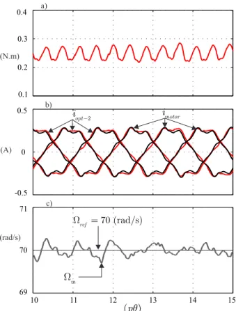
69 70 71 0.1 0.2 0.3 0.4 -0.5 0 0.5 10 11 12 13 14 15 (pq) 70 (rad/s) ref W = m W 2 opt i _- imotor (rad/s) (A) a) b) c) (N.m)

Fig. 16. Experimental performance of the PMSM speed control: a)

elec-tromagnetic torque, b) iopt−2 obtained and currents consumed by PMSM

imotor, c) rotor speed obtained

66 68 72 74

(rad/s)

Wobtained by the sinusoidal currents

Wobtained by 2 opt -i 70 76 64 10 11 12 13 14 15 (pq)

Fig. 17. Experimental speed obtained by the currents iopt−2 compared to the one derived by the sinusoidal currents

By using the proposed approach, the problem of torque and speed pulsation that is present in the control of conventional PMSMs have been solved.

VII. CONCLUSION

A new solution to calculate the optimal currents for non-sinusoidal multiphase PMSMs and particularly for three-phase non-sinusoidal machines has been presented in this paper. These optimal currents are derived from control strategies which depend on machine’s structure (for example, with or without the neural current). The optimization criterion consists of a desired constant torque and a minimal ohmic losses. These optimal currents are directly deduced from a geometrical development instead of calculations based on the Lagrange optimization. A new torque (or speed) control scheme has

been proposed. According to the learning capability of Adaline neural network, the optimal currents are obtained in real time. In each control scheme, the Adaline controller takes the place of the traditional torque or speed controller for ensuring the convergence of the motor’s torque or speed toward the desired one. The torque (or speed) ripple is efficiently compensated. This has been verified by various tests and comparisons under different conditions, even when one of the machine’s phases is faulty. The proposed simulations and experiments clearly confirm the high performances of our approaches.

REFERENCES

[1] T. M. Jahns and W. L. Soong, “Pulsating torque minimization techniques of permanent magnet ac motor drives - a review,” IEEE Trans. on Industrial Electronics, vol. 43, no. 2, pp. 321–330, 1996.

[2] H. R. Bolton and R. A. Ashen, “Influence of motor design and feed-current waveform on torque ripple in brushless dc drives,” IEE Proceedings on Electric Power Applications, vol. 131, no. 3, 1984. [3] S. Chen, C. Namuduri, and S. Mir, “Controller-induced parasitic torque

ripples in a pm synchronous motor,” IEEE Transactions on Industry Applications, vol. 38, no. 5, pp. 1273–1281, 2002.

[4] W. Qian, S. Panda, and J.-X. Xu, “Torque ripple minimization in pm synchronous motors using iterative learning control,” IEEE Trans. on Power Electronics, vol. 19, no. 2, pp. 272–279, 2004.

[5] M. Islam, S. Mir, and T. Sebastian, “Issues in reducing the cogging torque of mass-produced permanent-magnet brushless dc motor,” IEEE Trans. on Industrial Applications, vol. 40, no. 3, pp. 813–820, 2004. [6] G. Sturzer, D. Flieller, and J.-P. Louis, “Extension of the park’s

transformation applied to non-sinusoidal saturated synchronous motors,” European Power Electronics and Drives, vol. 12, no. 3, pp. 16–20, 2002. [7] ——, “Mathematical and experimental method to obtain the inverse modelling of nonsinusoidal and saturated synchronous reluctance mo-tors,” IEEE Trans. on Energy Conversion, vol. 18, no. 4, pp. 494–500, 2003.

[8] N. J. Nagel and R. D. Lorenz, “Rotating vector methods for smooth torque control of a switched reluctance motor drive,” IEEE Trans. on Industry Applications, vol. 36, no. 2, pp. 540–548, 2000.

[9] Y. Zhang, J. Zhu, W. Xu, and Y. Guo, “A simple method to reduce torque ripple in direct torque-controlled permanent-magnet synchronous motor by using vectors with variable amplitude and angle,” IEEE Trans. on Industrial Electronics, vol. 58, no. 7, pp. 2848–2859, 2011. [10] H. Zhu, X. Xi, and Y. Li, “Torque ripple reduction of the torque

predictive control scheme for permanent-magnet synchronous motors,” IEEE Trans. on Industrial Electronics, vol. 59, no. 2, pp. 871–877, 2012. [11] D. Wang, X. Wang, Y. Yang, and R. Zhang, “Optimization of magnetic pole shifting to reduce cogging torque in solid-rotor permanent-magnet synchronous motors,” IEEE Trans. on Magnetics, vol. 46, no. 5, pp. 1228–1234, 2010.

[12] R. Islam, I. Husain, A. Fardoun, and K. McLaughlin, “Permanent-magnet synchronous motor “Permanent-magnet designs with skewing for torque ripple and cogging torque reduction,” IEEE Trans. on Industry Applica-tions, vol. 45, no. 1, pp. 152–160, 2009.

[13] U.-J. Seo, Y.-D. Chun, J.-H. Choi, P.-W. Han, D.-H. Koo, and J. Lee, “A technique of torque ripple reduction in interior permanent magnet synchronous motor,” IEEE Transactions on Magnetics, vol. 47, no. 10, pp. 3240–3243, 2011.

[14] H. Le-Huy, R. Perret, and R. Feuillet, “Minimization of torque ripple in brushless dc motor drives,” IEEE Transactions on Industry Applications, vol. IA-22, no. 4, pp. 748–755, 1986.

[15] J. Y. Hung and Z. Ding, “Minimization of torque ripple in permanent magnet motors: a closed form solution,” International Conference on Industrial Electronics, Control, Instrumentation and Automation, vol. 1, pp. 459–463, 1992.

[16] ——, “Design of currents to reduce torque ripple in brushless permanent magnet motors,” IEE Proceedings on Electric Power Applications. Part B, vol. 140, no. 4, pp. 260–266, 1993.

[17] S. Clenet, Y. Lef`evre, N. Sadowski, S. Astier, and M. Lajoie-Mazenc, “Compensation of permanent magnet motors torque ripple by means of current supply waveshapes control determined by finite element method,” IEEE Trans. on Magnetics, vol. 29, no. 2, pp. 2019–2023, 1993.

[18] H. Kogure, K. Shinohara, and A. Nonaka, “Magnet configurations and current control for high torque to current ratio in interim permanent magnet synchronous motors,” in IEEE International Electric Machines and Drives Conference, vol. 1, 2003, pp. 353–359.

[19] A. P. Wu and P. L. Chapman, “Simple expressions for optimal current waveforms for permanent-magnet synchronous machine drives,” IEEE Trans. on Power Electronics, vol. 20, no. 1, pp. 151–157, 2005. [20] P. L. Chapman, S. D. Sudhoff, and C. A. Whitcomb, “Optimal current

control strategies for surface-mounted permanent-magnet synchronous machine drives,” IEEE Trans. on Energy Conversion, vol. 14, no. 4, 1999.

[21] K. Y. Cho, J. D. Bae, S. K. Chung, and M. J. Youn, “Torque harmonics minimisation in permanent magnet synchronous motor with back emf estimation,” IEE Proceedings on Electric Power Applications, vol. 141, no. 6, pp. 323–330, 1994.

[22] D. Grenier, L. A. Dessaint, O. Akhrif, and J.-P. Louis, “A park-like transformation for the study and the control of a nonsinusoidal brushless dc motor,” in Proceedings of IECON 21st International Conference on Industrial Electronics, Control, and Instrumentation, vol. 2, 1995, pp. 836–843.

[23] D. Grenier, L. A. Dessaint, O. Akhrif, Y. Bonnassieux, and B. Le Pioufle, “Experimental nonlinear torque control of a permanent-magnet syn-chronous motor using saliency,” IEEE Trans. on Industrial Electronics, vol. 44, no. 5, pp. 680–687, 1997.

[24] N. Matsui, “Autonomous torque ripple compensation of dd motor by torque observer,” in Asia-Pacific Workshop on Advances in Motion Control, 1993, pp. 19–24.

[25] P. Mattavelli, L. Tubiana, and M. Zigliotto, “Torque-ripple reduction in pm synchronous motor drives using repetitive current control,” IEEE Trans. on Power Electronics, vol. 20, no. 6, pp. 1423–1431, 2005. [26] X. Kestelyn and E. Semail, “A vectorial approach for generation of

op-timal current references for multiphase permanent-magnet synchronous machines in real time,” IEEE Trans. on Industrial Electronics, vol. 58, no. 11, pp. 5057–5065, 2011.

[27] W. Zhao, M. Cheng, K. T. Chau, R. Cao, and J. Ji, “Remedial injected-harmonic-current operation of redundant flux-switching permanent-magnet motor drives,” IEEE Trans. on Industrial Electronics, vol. 60, no. 1, pp. 151–159, 2013.

[28] D. Ould Abdeslam, P. Wira, J. Merckl´e, D. Flieller, and Y. A. Chapuis, “A unified artificial neural network architecture for active power filters,” IEEE Trans. on Industrial Electronics, vol. 54, no. 1, pp. 61–76, 2007. [29] N. K. Nguyen, P. Wira, D. Flieller, D. Ould Abdeslam, and J. Mer-ckl´e, “A comparative experimental study of neural and conventional controllers for an active power filter,” in 36th Annual Conference of the IEEE Industrial Electronics Society (IECON’10), Glendale, Arizona, USA, 2010, pp. 1995–2000.

[30] Z. Zhu and D. Howe, “Influence of design parameters on cogging torque in permanent magnet machines,” IEEE Trans. on Energy Conversion, vol. 15, no. 4, pp. 407–412, 2000.

[31] E. Favre, L. Cardoletti, and M. Jufer, “Permanent-magnet synchronous motors: A comprehensive approach to cogging torque suppression,” IEEE Trans. on Industry Applications, vol. 29, no. 6, pp. 1141–1149, 1993.

[32] L. Dosiek and P. Pillay, “Cogging torque reduction in permanent magnet machines,” IEEE Trans. on Industry Applications, vol. 43, no. 6, pp. 1565–1571, 2007.

[33] D. C. Hanselman, “Minimum torque ripple, maximum efficiency excita-tion of brushless permanent magnet motors,” IEEE Trans. on Industrial Electronics, vol. 41, no. 3, pp. 292–300, 1994.

[34] J. Y. Hung, “Design of the most efficient excitation for a class of electric motor,” IEEE Trans. on Circuits and Systems I: Fundamental Theory and Applications, vol. 41, no. 4, pp. 341–344, 1994.

[35] S. Dwari and L. Parsa, “An optimal control technique for multiphase pm machines under open-circuit faults,” IEEE Trans. on Industrial Electronics, vol. 55, no. 5, pp. 1988–1995, 2008.

[36] B. Widrow and E. Walach, Adaptive Inverse Control. Prentice-Hall, Inc., 1996.

Damien Flieller received the M.Sc. degree in Electrical Engineering from the Ecole Normale Sup´erieure (Cachan), France, in 1988 and the Ph.D. degree in Electrical Engineering from the University of Paris, France, in 1995. Since 1995, he is an Associate Professor in the Department of Electrical Engineering, INSA of Strasbourg, France. He is now director of the ERGE Group (Electrical Engineering Research Team). His research’s field are modeling and control of synchronous motors, active filter, and induction heating converters.

Ngac Ky Nguyen received his B.Sc degree in

Electrical Engineering from the Ho Chi Minh City University of Technology (HCMUT), Viet Nam in 2005. In France, he received his M.Sc. from Poly’Tech Nantes, in 2007 and his Ph.D. from the University of Haute Alsace (UHA), in 2010, both in Electrical and Electronic Engineering. From 2011 to 2012, he was with the Electrical Engineering Depart-ment, INSA of Strasbourg, France. Since September 2012, he is Associate Professor with the Laboratoire d’Electrotechnique et d’Electronique de Puissance de Lille (L2EP), Arts et M´etiers ParisTech. Lille Cedex, France. His research interests are the modeling and control of synchronous motors and power converters.

1501

Patrice Wira (M’04) received the M.Sc. degree

and the Ph.D. degree in Electrical Engineering from the University of Haute Alsace, Mulhouse, France, in 1997 and 2002, respectively. He received the Accreditation to Supervise Research (the French Habilitation `a Diriger des Recherches) in Computer Sciences from the University of Haute Alsace in 2009. He was an Associate Professor with the MIPS Laboratory (Laboratoire Mod´elisation, Intelligence, Processus, Syst`eme) at the University of Haute Al-sace. Since 2011, he is a Full Professor. He is author or coauthor of more than 20 technical papers covering his research interests from artificial neural networks for the modeling and simulation of complex automation systems, neuro-control approaches, to adaptive control systems.

Guy Sturtzerreceived the Ph.D. degree in Electrical Engineering from the Ecole Normale Sup´erieure, Cachan, France, in 2001. He joined the Depart-ment of Electrical Engineering, INSA de Strasbourg, France, where he is an Associate Professor. His main interests include electrical machines, power converters and renewable energies.

414

Djaffar Ould Abdeslamreceived the Ing. degree in Electronics Engineering from the University of Tizi-Ouzou, Algeria, in 2000, M.Sc. degree in Electrical Engineering from the University of Franche-Comt´e, Besanc¸on, France, in 2002 and the Ph.D. degree in ele ctrical engineering from the University of Haute Alsace (UHA), Mulhouse, France, in 2005. Since 2005, he is with the MIPS Laboratory, UHA, as an Associate Professor. His work concerns artificial neural networks, fuzzy logic and advanced control applied to power active filters and power electronics.

338

Jean Merckl´ereceived the M.Sc. and Ph.D.degrees in Electrical from University Nancy I, Nancy, France, in 1982 and 1988, respectively. In 1988, he joined the MIPS Laboratory, University of Haute Alsace, Mulhouse, France, where he participated in several adaptive signal processing projects. From 1991 to 1993, he was with the department of Electrical and Computer Engineering, University of California and San Diego, contributing to a 3-D optoelectronic neural architecture with efficient learning. He is currently a professor of Electrical and Computer Engineering. His research interests include adaptive neural computation with application to power electronic systems control.