Contribution to an extended modelling of the core flow behaviour in a rotor-stator cavity with a superimposed radial inflow

Science Arts & Métiers (SAM)

is an open access repository that collects the work of Arts et Métiers Institute of Technology researchers and makes it freely available over the web where possible.

This is an author-deposited version published in: https://sam.ensam.eu

Handle ID: .http://hdl.handle.net/10985/9697

To cite this version :

Roger DEBUCHY, Andréa RINALDI, Gérard BOIS, Florin BREABAN - Contribution to an extended modelling of the core flow behaviour in a rotor-stator cavity with a superimposed radial inflow - mechanics and industry - Vol. 16, n°4, p.12 - 2015

Any correspondence concerning this service should be sent to the repository Administrator : archiveouverte@ensam.eu

CONTRIBUTION TO AN EXTENDED MODELING OF THE CORE

FLOW BEHAVIOUR IN A ROTOR-STATOR CAVITY WITH A

SUPERIMPOSED RADIAL INFLOW

DEBUCHY Roger (1, *)_{, RINALDI Andréa}(2)_{, BOIS Gérard} (3)_, BREABAN Florin (1)

1 _{Laboratoire Génie Civil & géo-Environnement (LGCgE- EA 4515), UArtois/FSA Béthune, F-62400}

Béthune, France

2

CRITTM2A-62700 Bruay la Buissière

3 _{Laboratoire de Mécanique de Lille (LML – UMR 8107), Arts et Métiers ParisTech, Lille, France}

*_{Corresponding author: roger.debuchy@univ-artois.fr}

Abstract

The present study focuses on the turbulent flow with separated boundary layers in a rotor-stator cavity with a low aspect ratio subjected to a weak centripetal radial inflow. One of the major results is to show, with the help of numerous experimental data, that the core swirl ratio always evolves according to a power law of the dimensionless radius. Starting from this simple behaviour law, new original flow properties are highlighted and particularly the existence of an invariant quantity in the core region.

Nomenclature

qp

C peripheral dimensionless coefficient of flow rate, =Ro G Re1 5

qr

C _{dimensionless coefficient of flow rate,} 1 5 * 13 5

(

₂ 3

)

= Re q r − πΩR

Ek Ekman number, ₁ 2

= ReG G gap ratio, H R=

h peripheral opening of the cavity H axial gap of the cavity

K core swirl ratio, * *

V_θ r

= at *

z = 0

B

K core swirl ratio in case of solid body rotation

p

K pre-swirl ratio, K= at r* =1

p _{static pressure on the stator}

atm

p atmospheric pressure

*

P dimensionless static pressure on the stator,

(

1 2 2

)

atm 2 R

p p

= − ρΩ

q _{volume flow rate}

*

Q dimensionless flow rate coefficient, =q

ν

r

r radial coordinate

*

r dimensionless radial coordinate, r R=

0

*

R radius of the rotor

H

R outer radius of the hub Re _{Reynolds number,} 2 R = Ω ν Ro _{Rossby number,} 2 q 2

πΩ

R H = r, , z

v v v_θ radial, tangential and axial mean velocity components * *

r ,

V V_θ dimensionless radial and tangential velocity components,

r ,

v R v_θ R

= Ω Ω

* z

V dimensionless axial velocity, =v G Rz Ω

2 i i j v' , v' v' turbulent correlations ( i, j r, ,z ; i= θ ≠ j ) * * 2 i i j

v' , v' v' dimensionless turbulent correlations

(

)

2 2*

(

)

2 * i i j G ΩR v' G ΩR v' v' = , = ( i, j r, ,z ; i= θ ≠ j ) z axial coordinate *

z dimensionless axial coordinate, z H=

α

constant in the present theoretical model

α

value of the constant

α

computed from empirical relationships

0

α

value of the constant

α

in the case of an isolated cavity

ε

_{function of} *

z in the present theoretical model

Ψ dimensionless parameter

K

∆ error in the calculation of K Ω angular speed of the rotor

1 Introduction

The knowledge of the behaviour of rotating flow has been the main objective of many experimental, numerical and theoretical studies over the past decades. Natural and oceanic movements, atmospheric phenomena, as well as flow inside hard disk data storage, numerous examples are linked to this kind of flow. In such a range of possible aspects, the present paper deals with the domain of operating conditions of rotating machineries. Often, in turbomachinery applications, the flow between the rotating parts such as impeller and disks is subjected to a forced rotation. In gas turbines, turbojets, centrifugal multistage compressors, severe operating conditions expose the moving walls to high level of stress and excitation. These phenomena can lead to reliability problems and even to destruction if they are not correctly controlled. Therefore, the knowledge of the dynamic fluid properties in the inter-disk spacing is of major interest for the pump and gas turbine designers in order to improve performances as well as security and working life. In the cooling systems of actual machines, the moving walls rotate near to a fixed shroud or to others co or contra-rotating walls. Although these geometries are complex, they are often addressed through simplified rotating disk systems, which are of great interest both from mathematical and practical point of view. Indeed, theoretical solutions can be found starting from the Navier-Stokes equations entering in the domain of classical differential equations’ integration. Many reference books have been

devoted to the question, among which those of Dorfman [1], Owen and Rogers [2, 3] and more recently Poncet [4].

In the present paper, attention is focused to the turbulent flow in a rotor-stator system with a low aspect ratio, where the flow exhibits three domains: two boundary layers near the disks separated by a core region. The prediction of the core swirl ratio K , defined by the ratio between the tangential velocity of the fluid in the central core and the local velocity of the rotating wall, is a great challenge for the designers because this dimensionless quantity is linked to the pressure coefficients inside the cavity. It is the reason why numerous theoretical, experimental and numerical studies have been devoted to this question. We can quote the studies by Kurokawa and Toyokura [5], Poncet et al. [6, 7] as well as Innocenti et al. [8]. In these studies, it was assumed that there is no fluid exchange outside the boundary layer, which seems to be inconsistent with experimental observations. This point has been improved by Abdel Nour et al. [9, 10]. Note that Debuchy et al. [11, 12] have also led to analytical solutions including the three components of velocity and the radial distribution of the static pressure in a rotor stator system opened to the atmosphere at the periphery, without any radial superimposed flow or subjected to a centripetal inflow rate. The common feature of all the theoretical works mentioned above is that the analytical solutions were obtained under the assumption that turbulence has no significant effect in the core region despite the flow is turbulent.

The present work is based mainly on the analysis of numerous experimental results, one the one hand data obtained in the studies we have conducted on the

subject [9-12, 16], on the other hand results extracted from the literature [6, 7]. Our contribution is to provide the simplest possible modelling of the radial distribution of the core swirl ratio and therefore of the static pressure inside the cavity. New typical properties of the central core that arise directly from this behaviour law are also highlighted. From a theoretical point of view, these results are consistent with the Navier-Stokes equations only under certain assumptions and conditions. This theoretical approach of the problem, which is not the main issue of this paper, is appended to the paper.

Thus, the remaining of the paper is organized as follows. The scope of the present study is specified in section 2. This section also includes a description of the experimental apparatus and test conditions. The overall results, the original flow properties as well as a new behaviour law for the central core swirl ratio are discussed in Section 3. The main conclusions and perspectives of this work are given in section 4.

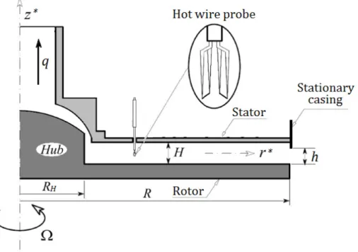
2 Scope of the study – Experimental apparatus

The study focuses on the flow in an annular cavity between two parallel and coaxial disks (Figure 1). The disk located at z = - H 2 rotates at a constant speed Ω (rotor). It is equipped with a central hub of radius R_Hwhich represents the axis

of an actual machine. From a theoretical point of view, this hub avoids the singularity at r = . The disk located at0 z = H 2 is fixed (stator). The cavity is

opened to the atmosphere at the periphery. The fluid is assumed to be incompressible and isothermal. This problem has been addressed in [11].

The main dimensionless parameters are the gap ratio of the cavity G and the Reynolds number defined by:

2

G=H R ; Re=

Ω

R

ν

(1)

The structure of the flow in an annular rotor-stator cavity has been often studied in the past. In particular, the classification established by Daily & Nece [13] revealed four distinct flow regimes, laminar or turbulent and with separated or merged boundary layers (Figure 2). The main characteristics are depicted as it follows: • both laminar flow regimes are separated by a curve fitting 11/ 5

Re G ≈2.9 ; • the transition from laminar to turbulent when the boundary layers are

separated by a core region occurs when the Reynolds number is around

5

Re≈1.58 10× ;

• the common limit between the turbulent flow regimes satisfies the equation

16 / 3 3

Re G ≈7.8 10× − whereas the common limit between the flow regimes with merged boundary layers corresponds to the following condition 10 / 9

Re G ≈366 ;

• the common limit between the flow regimes II and III fits the curve

16 / 15 6

In the present work, attention is focused on the region IV of this classification. The authors assume that The Ekman number defined by

(

2

)

1

Ek = Re G − remains small with regards to unity so that the flow is turbulent and the boundary layers are separated by a central core region according to Dyment [14].

In addition, the rotor-stator cavity is connected near the axis to a vacuum system generating a weak superimposed centripetal volume flow rate q , as in [12]. The dimensionless flow rate parameter is the Rossby number defined by:

(

)

(

)

Ro=U

Ω

R ; =U q 2 RH

π

(2)

In the present work, the centrifugal effects remain predominant with respect to the radial inlet effects so that Ro<< . The flow structure properties depicted in 1

Figure 2, valid in the case of an isolated cavity i.e. without any superimposed flow, are not affected by a weak radial superimposed inflow.

Let us summarize the assumptions relating to the different dimensionless parameters:

Re>> ; << ; 1 G 1 Ek<< ; 1 Ro<< 1 (3)

The experimental apparatus has already been described in several studies [9-12]. The annular cavity is delimited by two parallel and coaxial discs separated by an axial gap H adjustable up to 0 0375. . The lower disc with a radius R equal m

to 0 375. , rotates with an angular velocity which can be varied up to 2000 rpmm

2000 rpm. It is situated at z= −H 2. It was equipped with a central hub the radius of which beingRH =0 09. . The upper disk situated at m z=H 2was fixed. Note that the mid-height of the cavity corresponds to z 0= . At the periphery, the cavity was opened to the atmosphere.

Velocity measurements between the discs were performed in ambient air conditions with the help of a specific hot-wire probe made of two perpendicular

m

µ

5 wires situated in the same plane. Each sensor was connected to a DANTEC 55M25 anemometry device.

During the experiments, the probe was introduced inside the cavity through the stator and moved in the axial direction. The angular position of the probe was remained fixed, with the two wires positioned at ± 45° regarding to the tangential direction. This technique was used in order to provide the radial and tangential mean velocity components. Additional details about the experimental apparatus can be found in [9].

The accuracy of the circumferential velocity measurement is related to several factors:

- the calibration of the probe. In the present work, it was performed in a specific wind tunnel. For each sensor, the coefficients of the King’s law were computed in order to provide the best fit between the flow velocity measured by a pitot tube and the anemometer voltage output. During this step, the uncertainty for each sensor effective velocity was estimated to be ± 2%.

- The initial position of the probe between the disks. The calculation of tangential mean velocity in the post-processing of the data requires the initial position of the sensors to be exactly ± 45° regarding to the tangential direction. This setting is difficult to achieve exactly, with the consequence that the uncertainty for the calculation of the tangential mean velocity is ± 2%.

- The assumption in the post-processing of the data. The tangential velocity component was deduced from the effective velocities of the two sensors with the help of analytical relationships using the assumption that the axial velocity is zero. We consider that this assumption leads to a negligible error.

Finally, the overall measurement uncertainty for the circumferential velocity component is estimated to be ± 4%.

The experimental conditions and the values of the dimensionless parameters are detailed in Table 1.

3 Results and discussion

In the remainder of the paper, all results will be presented using the dimensionless quantities (with superscript *) defined by Eq. (A1) in the appendix.

In a first step, the attention is drawn to the modelling of the core swirl ratio K , defined by * *

K =V_θ r at *

z = , which is significant physical quantity for turbine 0

Indeed, in the case of a turbulent flow with separated boundary layers, the axial pressure gradient is zero so that the dimensionless static pressure and the core swirl ratio are related by the radial equilibrium equation * * 2 *

dP dr =2K r (see Appendix). Then, the objective is to provide a physical law for the radial distribution of core swirl ratio, which should allow quantifying the axial thrust inside the cavity and highlighting new physical properties for the core region, which is an important issue to our opinion. Our approach is based on numerous experimental observations to support our conclusions. In addition, for the reader interested in the theoretical aspect of the problem, the results are always enhanced by an analysis based on an asymptotic development. However, as this is not the main objective of this work, this theoretical part is given in the appendix.

The first significant observation in this paper is that all experimental results outlined in Table 1 fit a simple behaviour law of the form:

* p

K =K r −α (4)

This relationship reveals two quantities to be determined, the peripheral core swirl ratioKp which is defined by

*

V_θ at z* = and 0 *

r = as well as the value of the 1

power

α

which depends on the experimental conditions and requires to be adjusted for each test case.

In the present analysis, the pre-swirl ratio had to be estimated by extrapolation because no measurement could be performed at *

r =1.0. To overcome this

(

* *

)

1 1

K K = r r −α, where * 1

r corresponds to the largest value of r* where

measurements have been performed and where K₁ is the core swirl ratio at r₁*.

For the experimental results extracted from [9], * 1

r =0.88. Figure 3 provides a double logarithmic representation of Log K K

₍

₁

₎

versusLog r r

(

* ₁*

)

,

corresponding to a linear evolution. For each test case, the slope of the curve gives the value of the power

α

and the pre-swirl ratio Kp is deduced from the

following relationship *

p 1 1

K =K r α. The values are given in Table 2.

A major consequence of this result arises because Eq. (4) can also be written on the following form:

5 13 qr p qp C K K C α   = _ _   (5)

whereC_qris the dimensionless flow rate coefficient introduced by Poncet [6, 7]

and Cqp the peripheral value ofCqr. These parameters are defined as it follows:

1 5 ₁₃ * ₅ qr 3 Re C q r 2

π Ω

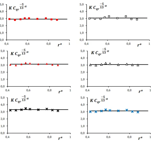
R − = , 1 5 qp C =Re G Ro (6)

Eq. (5) is of particular interest because it implies that the following quantity remains constant: 5 5 13 13 qr p qp K C α K C α cons tan t − − = = (7)

The values of 5 13 qr K C α −

were computed for each radial location and the line corresponding to the peripheral value

5 13 p qp

K C α

−

were plotted in Fig. 4 for the test cases corresponding to G 0.053= . The results clearly highlight that the dimensionless quantity defined in Eq. (7) remains constant. Even if the results are not presented, Eq. (7) has been checked to be valid for all test cases depicted in Table 1.

At the periphery of the cavity, the value of the quantity

5 13 p qp K C α − depends on both the pre-swirl ratio and the dimensionless parameter C_qp which have a physical

signification. It also depends on

α

which is unknown a priori. Therefore, a correlation between the values of

α

reported in Table 2 and the dimensionless parameters of the problem has been established. This is going to be presented in the following part of this paper.

At this stage of the discussion, our attempt is to find an empirical relationship between the adjusted values of

α

reported in Table 2 and the parameters of the problem (the Reynolds number, the gap ratio, the Rossby number as well as the pre-swirl ratio). Subsequently in the paper, the values computed from this relationship will be denoted

α

. Index 0 will be added in the case of a rotor-stator cavity without any superimposed flow. This particular case will be called “isolated cavity”.

For the isolated cavity

₍

Ro=0

₎

, the recent work [16] showed that the flow

behavior can be modeled by the relationship (4), at least in a peripheral region, provided that the pre-swirl ratioK_pis low. In this work, the value of the power in

the solution (4) was computed from the following empirical relationship:

0.52 0 2.31 ( K_B K )_p

α

= × − . The core swirl ratioK_Bcorresponding to the solid body

rotation was fixed to 0.38 , which correspond to the theoretical value mentioned in [3]. For fixed values of the gap ratio and Reynolds number, the value of the power

α

must vary very slightly and continuously as soon as the cavity is subjected to a very weak superimposed flow rate

(

Ro→0

)

. Consequently, we

proposed an empirical law of the form

α

=

α

0+ f (Re,G,Ro, K )_p . The f function

depends on the main dimensionless parameters defined in Eqs (1) and (2), but also likely to geometrical parameters related to the layout of the cavity. With regard to the geometrical parameters relating to the periphery of the cavity, they were taken into account by means of the pre-swirl ratioK_p. Other parameters related to the

geometrical shape of the cavity close to the hub or to the discs roughness, among others, may also interfere with the flow behavior and therefore in the f function. They were not considered in the present paper.

Based on the values reported in Table 2, it can be observed that

α

increases as Ro increases for a fixed value of the Reynolds number. As an example among other, we can compare the adjusted values of tests 1 and 2. Instead,

α

is a decreasing function of the gap ratio for fixed values of the Rossby and Reynolds

numbers (see test cases 1 and 7). Thus, in order to provide adequate results with the

α

values listed in Table 2, we proposed the following empirical law:

0.52 3 p p 2.31( 0.38 K ) 1.67 10 K

α

_{≈ − + ×} −

Ψ

_, 1/ 2 3 / 2 3 / 4 Re G Ro

Ψ

₌ − ₍₈₎

For each test case, the difference between

α

and

α

is reported in Table 2. It is at most equal to 0.06 , which means that the values of the power

α

in Eq. (4) can be computed with the help of the empirical relationship (8) with an accuracy better than 5%, for all the experimental conditions depicted in Table 1.

In Figures 5 and 6, we compared the radial distributions of the experimental core-swirl ratio to that computed from the combination of Eq. (4) and Eq. (8), with the value of the pre-swirl coefficientK_p indicated in Table 2. The adequacy between

experiment and theory is very good both for G 0.053= and G 0.08= . Using Eqs (4) and (8), the error in the calculation of K is mainly related to the error in the pre-swirl ratioK_p. When the cavity is opened to the atmosphere, recirculation

phenomenon can be observed in a peripheral area where the flow is not established, so that it remains difficult to estimate the Kpvalue with a good

accuracy.

Starting from Eqs (4) and (8), the estimation of the error K

∆

in the computed

value of K is

∆

K = A×

∆

K_p , with _{Ln( r )}*

{

(

)

0.48 _{3 *}

}

p p A e− α 1 K  1.20 0.38 K − 1.65 10−

Ψ

Ln( r ) = − _− × − + × _   . For

each test case, this error depends on the level of the pre-swirl ratio, the main dimensionless parameters defined in (1) and (2) and the dimensionless radial position. The computed values of K

∆

are indicated in Table 2 (last column) for

*

r =0.43, which corresponds to the lowest radial position where the measurements were carried out, and for ∆Kp =0.01.

Up to now, the discussion focused on the modeling of the core swirl ratio. However, numerous studies have shown that the axial gradient of the tangential velocity component is not zero, especially when the cavity is subjected to a superimposed radial inflow. As an example, this is the case of the experimental results in [12]. Thus, in a next part of the discussion, it seemed interesting to test an analytical solution providing the axial profile of the tangential velocity component * V_θ of the form: * * * p V_θ r =K r −αg (9) where g is a function of *

z satisfying g 0

( )

=1, so that, at mid-height of the cavity

Eq. (9) is consistent with the analytical solution (4). If considering that the axial gradient of *

V_θ is small compared to unity, this latter

equation can be written in the following form:

(

)

* * * *

p

where b is a constant.

This simple analytical solution provides an explanation to major experimental findings in [12].

For the isolated cavity ( Ro 0= ), it was assumed that the axial gradient of the tangential velocity is sufficiently low to consider that b 0= . It was also showed in [16] that a balancing process of the flow inside the boundary layers occurs when the pre-swirl ratio is low, which implies that the central core swirl ratio is a decreasing function of *

r , at least in a peripheral region. This behavior ends as

soon as the flow rates inside the boundary layers balance each other. Then, the core rotates as a solid body. The authors in [16] showed that two behavior laws coexist provided that the radial extension of the cavity is sufficiently large:

(

)

0 0 1/ * * * * * * * * * * B B p B p r ≤r :V_θ r =0.38 ; r ≥r :V_θ r =K r −α ; r = K 0.38 α (11)

This last relationship is valid in the case of an isolated cavity

(

Ro=0

)

, so that the

values of

α

0is obtained with the help of Eq. (8) with Ψ = . 0

When there is a weak superposed radial inflow so that Ro→ , the axial 0

gradient of the tangential velocity is no longer zero so that b 0≠ in Eq. (10). The analytical solution (10) is consistent with the following observation made by Debuchy et al [12]: the weakest superimposed flow does not lead to major

changes near the periphery of the rotor-stator system, but becomes predominant when approaching to the axis.

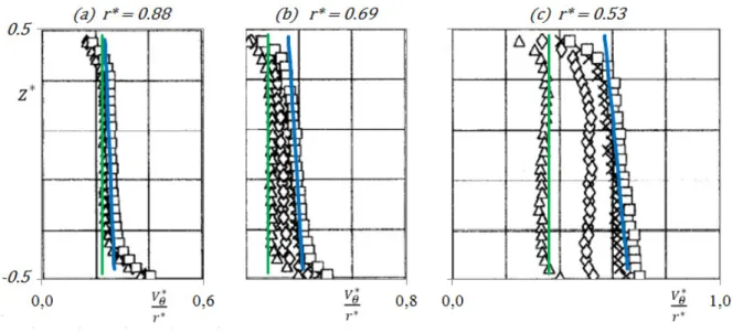
Figure 7 provides a validation of Eq. (10) and Eq. (11) with the help of experimental results extracted from [12] for 6

Re=1.47 10× and G 0.08= . We compared two test cases corresponding to the isolated cavity ( Ro 0= ) and

Ro≈0.0167. In both cases, the pre-swirl ratio was estimated to be approximately equal to 0.20 and the value of b was fixed to 0.12− . For the isolated cavity, Eq. (8) gives

α

0 =0.94which allows to predict that the solid body rotation of the core

appears for *

r ≤0.51. When a superimposed inflow corresponding to Ro≈0.0167is assigned, Eq. (8) gives

α

=1.78. The difference between the core

swirl ratio with and without superimposed throughflow is about 11% at

*

r =0.88(Fig. 7a), 37% at *

r =0.69(Fig. 7b) and reaches 70% at *

r =0.53 (Fig. 7c). This difference becomes much higher for *

r ≤0.51, because K remains

constant when Ro 0= whereas it always increases as *

r decreases for Ro≈0.0167.The present theory is consistent with the results extracted from [12].

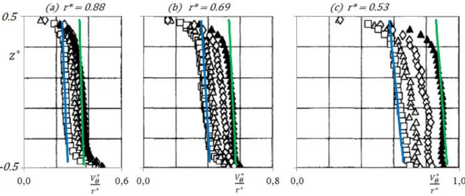
We also compared the present theory to experimental results extracted from [12] obtained in a rotor-stator cavity with a partial peripheral opening (Fig. 8). As

h / H decreases, the peripheral inlet area is shifted towards the rotor, with the

consequence that the pre-swirl ratio K_p increases. In Figure 8, we focused on the

experimental results for two values of the peripheral opening coefficients

h / H =1.00 and h / H 0.25= , G=0 08. , 6

Re=1.47 10× and Ro 0.0167≈ . For h / H 0.25= , the pre-swirl coefficient is approximately equal to 0.28 , which

gives

α

=1.85 according to Eq. (8). The results presented in Figure 8 show that the theoretical model corresponding to Eq. (10) is realistic.

The combination of the simple behaviour law (4) and the empirical relationship (8) represents to our opinion a significant advance as the radial distribution of the core swirl ratio can be computed with a good accuracy on one test rig and over a wide range of variation of the main dimensionless parameters, provided that the pre-swirl ratioKp is known. Of course, we do not expect that

this theory is universal because, as mentioned above in the paper, all dimensionless parameters have not been considered. However, in this last step of the discussion, our aim is to check that the same approach can be used for other configurations extracted from the literature. For this purpose, we selected the results obtained by Poncet et al. [6, 7]. The major difference is the high level of the pre-swirl ratioKp, which is linked to the peripheral geometry of the cavity.

Especially, the level of the pre-swirl ratio Kp is higher than that of the theoretical

core swirl coefficient in the case of solid body rotation

(

KB =0.38

)

.Consequently, when the cavity is isolated, we can predict that the

core swirl ratio is an increasing function of *

r in a peripheral region, which

indicates that the value of

α

0 is necessarily negative. We argue subsequently that

this value can be determined by the relationship: α0 = −2.31× K_B −K_p 0.52. The

experiments extracted from the work performed by Poncet et al. [6] were used in order to find an empirical law of the form α =α0+ f (Re, Ro,G,K )_p . The best fit

for the radial distribution of the core swirl ratio was obtained with the combination of Eq. (4) and the following empirical relationship:

p 0.52 _{4 1.4} p 2.31 0.38 K 1.18 10 K α _{≈ − × − + ×} − Ψ _, 1/ 2 1 Re G Ψ ₌ − ₍₁₂₎

The experimental conditions and the values of K_pand

α

are summarized in Table 3. Note that the dimensionless flow rate coefficient *

Q which was used by

Poncet et al. in [6] is defined by *

Q =q ν , so that r *

Q =2π⋅Ro Re G⋅ ⋅ . Figure 9(a) shows a very good agreement between the theoretical and experimental radial distributions of the core swirl ratio.

We have also verified that the radial equilibrium equation

* * 2 *

dP dr =2K r combined with Eq. (4) remains available to provide an analytical

law for the radial pressure distribution. The corresponding solution can be written as it follows:

(

2( 1 ) 2( 1 )

)

0 2 p * K * * P r r ( 1 ) α α

α

− − = − − (13) where 0 *

r is the radial location corresponding to a dimensionless static pressure

equal to zero.

Figure 9(b) shows a comparison between the radial distribution of the dimensionless static pressure measured by Poncet et al. [6] and the theoretical

data computed with the help of Eqs (12) and (13). In both cases, the pressure level is adjusted to 0 at the dimensionless radial location *

0

r =0.92. The agreement of the results is very good, which means that the axial gradient of the tangential velocity component included in the function g in Eq. (9) has no major influence on the pressure distribution.

4 Conclusions

The object of the present study was to investigate the turbulent flow in a rotor-stator cavity with a low aspect ratio subjected to a centripetal radial inflow. All results are valid in the core region of the flow existing between the two separated boundary layers (flow regime IV according to the classification by Daily and Nece [13])

Starting from numerous experimental data, a simple behaviour law for the radial distribution of the central core swirl ratio has been highlighted: K varies according to a power law of the dimensionless radius. This solution requires the knowledge of two quantities: the pre-swirl ratio of the fluid at the periphery of the rotor-stator system which is a boundary condition and the value of the power. For this latter quantity, the authors have found an empirical relationship that provides good results for one test rig and over a wide range of the significant dimensionless parameters. For now, this relationship can not be generalized to all test rigs, probably because geometrical parameters related to the inner part of the cavity have not yet been taken into account. This is one of the future works.

Nevertheless, the present behaviour law is in excellent agreement with numerous experiments from the literature. It also leads to the radial distribution of the static pressure and highlights the existence of an invariant quantity in the core region.

This experimental analysis has been complemented by a theoretical work. The aim was to specify the assumptions which ensure that the present analytical solution remains consistent with the Navier-Stokes equations. Nevertheless, as this part was not the main interest of this study, it is presented in the Appendix. In particular, it is shown that turbulence cannot be totally neglected in the central core of the flow. It results that additional data are needed to support these assumptions. Thus, one of the perspectives of the present work is to analyse numerical results including all components of the Reynolds tensor, which may be useful to propose a simple modelling of the Reynolds tensor effects for engineering applications. Then, the present results could be extended to the case of complex peripheral conditions such as small radial turbomachinery components and could be developed for the optimising of the modern turbo-compressors in automotive field.

REFERENCES

[1] L. A. Dorfman. Hydrodynamics resistance and the heat loss of rotating solids. Oliver and Boyd, Edinburgh, 1963

[2] J. M. Owen, R. H. Rogers. Flow and heat transfer in rotating-disc system, vol. 1: rotor-stator system. Ed W D Morris, John Wiley & Sons Inc, 1989

[3] J. M. Owen, R. H. Rogers. Flow and heat transfer in rotating-disc system, vol. 1: rotating cavities. Ed W D Morris, John Wiley & Sons Inc, 1995

[4] S. Poncet. Écoulements de type rotor-stator soumis à un flux axial : de Batchelor à Stewartson. Editions universitaires européennes, 2010

[5] J. Kurokawa, T. Toyokura. Study on axial thrust of radial flow turbomachinery. 2nd Intl JSME Symp. Fluid Machinery and Fluidics, Tokyo, 4–9 September,1972, 2: 31

[6] S. Poncet, M. P. Chauve, P. Le Gal. Turbulent rotating disk flow with inward throughflow. Journal of Fluid Mechanics, 522 (2005) 253-262

[7] S. Poncet, M. P. Chauve, P. Le Gal. Lois analytiques pour les écoulements en cavité rotor-stator. Mécanique & Industries 9 (2008) 227-236

[8] L. Innocenti, M. Micio, R. Da Soghe, B. Facchini. Analysis of gas turbine rotating cavities by an one dimensional model. Isromac Paper 12, 2008

[9] F. Abdel Nour, A. Rinaldi, R. Debuchy, G. Bois. Influence of a weak superposed centripetal flow in a rotor-stator system for several pre-swirl ratios. International Journal of Fluid Machinery and Systems, 5 (2012) 49-59

[10] F. Abdel Nour, S. Poncet, R. Debuchy, G. Bois. A combined analytical, experimental and numerical investigation of turbulent air flow behaviour in a rotor-stator cavity. Mécanique & Industries 10 (2009) 195-201

[11] R. Debuchy, F. Abdel Nour, H. Naji, G. Bois. Investigation of the fluid flow in an isolated rotor-stator system with a peripheral opening. Science in China

Physics,Mechanics & Astronomy, 56-4 (2013) 745-754

[12] R. Debuchy, A. Dyment, H. Muhe, P. Micheau. Radial inflow between a rotating and a stationary disc. European journal of Mechanics-B/Fluids 17 (1998) 791-810

[13] J. W. Daily, R. E. Nece. Chamber dimension effects on induced flow and frictional resistance of enclosed rotating disks. J Basic Eng 82 (1960) 217-232. [14] A. Dyment. Formulation asymptotique des écoulements d’un fluide incompressible entre deux disques coaxiaux voisins en rotation. C. R. Acad. Sci. Paris, Série II 292 (1981) 129- 132

[15] G. K. Batchelor. Note on a class of solutions of the Navier–Stokes equations representing steady rotationally-symmetric flow. J Mech Appl Math, 4 (1951) 29-41

[16] R. Debuchy, F. Abdel Nour, G. Bois. An analytical modeling of the central core flow in a rotor-stator system with several pre-swirl conditions. J. Fluids Eng., 132-6 (2010) 061102

Table Test Symbol G

10

−6

_×

_Re

10 Ro

3

_×

10

3

×

C

_qp 1 0.053 1.03 5.69 4.84 2 0.053 1.03 8.54 7.26 3 0.053 1.47 3.98 3.63 4 0.053 1.47 5.97 5.45 5 0.053 1.95 4.51 4.36 6 0.053 1.95 5.64 5.44 7 0.08 1.03 5.69 7.26 8 0.08 1.03 7.59 9.68 9 0.08 1.47 3.98 5.45 10 0.08 1.47 5.30 7.27 11 0.08 1.95 4.01 5.81 12 0.08 1.95 5.01 7.26

Test

K

p

α

α

K

∆

1 0.14 1.50 1.50 0.04 2 0.14 1.64 1.64 0.05 3 0.13 1.47 1.46 0.04 4 0.13 1.59 1.58 0.05 5 0.12 1.57 1.54 0.04 6 0.12 1.61 1.61 0.05 7 0.10 1.30 1.35 0.03 8 0.10 1.35 1.38 0.03 9 0.09 1.28 1.34 0.03 10 0.09 1.32 1.37 0.03 11 0.08 1.38 1.37 0.03 12 0.08 1.42 1.39 0.03 Table 2: values of the constants in the model

G

10

−6

_×

_Re

Q

*

K

p

α

0.024 1.04 2579 0.46 1.07 0.024 1.04 5159 0.54 1.23 0.024 1.04 10317 0.62 1.47 0.036 2.08 10317 0.54 1.10 0.048 4.15 10317 0.46 1.07 Table 3: experimental conditions in [6]

Figures

0,0 0,5 1,0 1,5

-1,00 -0,50 0,00

Figure 3: experimental validation of the behaviour law

(

* *

)

1 1

K K = r r −α.

Figure 4: experimental validation of the behaviour law (7).

Present experimental results extracted from [9]: see the symbols in Table 1 : value of 5 13 p qp K C α −

Figure 5: radial distribution of the core swirl ratio - G=0 053.

Experimental results extracted from [16]: see the symbols in Table 1 ; : Eq. (4) with the computed values of

α

according to Eq. (8)

Figure 6: radial distribution of the core swirl ratio - G=0 08.

Experimental results extracted from [16]: see the symbols in Table 1 ; : Eq. (4) with the computed values of

α

according to Eq. (8)

Figure 7: Validation of Eqs (10) and (11) Dimensionless tangential velocity profiles

0 08

G= . , 6

Re=1.47 10× , K_p =0.20

Experimental results extracted from [12]: isolated cavity, Ro 0.0167≈ : Eq. (10) with

α

=1.78and b= −0.12 ; : Eq.(11) with

α

0 =0.94

Figure 8: Validation of Eqs (10) and (11) Dimensionless tangential velocity profiles

0 08

G= . , 6

Re=1.47 10× , Ro 0.0167≈

Experimental results extracted from [12]: h / H 1.00= ; h / H 0.25= : Eq. (10) with K_p =0.20,

α

=1.78and b= −0.12

Figure 9: Validation of the present behaviour law with the experiments by Poncet et al. [6]

APPENDIX

In the appendix, all equations and results will be presented using the dimensionless quantities (with superscript *) defined by:

(

)

(

)

(

)

* * * * * r r z z 2 _* 1 atm 2 * 2 2 2 i i * 2 i j i j r Rr ; z GRz ; v RV ; v RV ; v G RV p p R P v' G R v' ( i r , , z ) v' v' G R v' v' ( i, j r , , z ; i j ) θ θ

Ω

Ω

Ω

ρ Ω

Ω

θ

Ω

θ

= = = = = − = = = = = ≠ (A1)

It was assumed that all turbulent correlations have the same order of magnitude. Using the dimensionless quantities defined in Eq. (A1) with the assumptions (3), the conservation of mass and Navier-Stokes equations become:

(

* *

)

(

* *

)

r z * * * *2 * * * * r * r r z r * z * * * * * * * * * * * r z r * z * * * * * r V r V 0; r z V V V 1 dP v' v' V V ; r z r 2 dr z V V V V v' v' V V ; r z r z P 0 z θ θ θ θ θ ∂ ∂ + = ∂ ∂ ∂ ∂ ∂ + − = − − ∂ ∂ ∂ ∂ ∂ ∂ + + = − ∂ ∂ ∂ ∂ = ∂ (A2)

Thus, the last relation in Eq. (A2) shows that the axial pressure gradient inside the cavity is zero.

One particular solution was given by Batchelor [15] in the case of infinite disks. In the central core region, when assuming that the turbulence is null, the flow rotates as a solid body, which corresponds to the following solution:

* r V = , 0 * * B V_θ =K r , * z V = , 0 (A3)

The axial gradient of the tangential velocity component is null. The core swirl ratio K defined by * *

K =V_θ r remains a constantKB. The radial pressure

distribution can be easily deduced with respect to a constant from the radial equilibrium equation * * 2 *

B

dP dr =2K r which comes from the second relation of Eqs (A2).

When the radial extension of the discs is finite and the annular cavity opened to the atmosphere at the periphery, the radial velocity component is no longer equal to zero, moreover when a radial inflow is superimposed.

Then, let us focused on the third relation in Eq. (A2) which was always neglected in the studies [5-11] quoted in the introduction.

When it is assumed that the axial gradient of the tangential velocity component is insignificant so that *

V_θ is only a function of r* and also that the turbulence is

negligible in the core region, this equation becomes * * * *

dV_θ dr +V_θ r = , which 0

leads to the solution * * 1 p

V_θ =K r − . The constantKp, which is called the peripheral

swirl ratio or pre-swirl ratio, comes from the boundary conditionK =K_pat *

Consequently, the core swirl ratio evolves as a power law in *

r of the form

* 2 p

K =K r − . This solution indicates that the core swirl ratio increases as *

r

decreases, which is consistent with all experimental observations [9-12] in the case of a cavity subjected to a weak centripetal flow. Nevertheless, the value of the power can not always be set to -2 because it has already been observed in [12] that K increases as Ro increases for a fixed value of the pre-swirl ratioKp. It is

the reason why the authors suggested the solution (4) for the radial distribution of core swirl ratio. In addition, numerous experimental results in [12] have shown that the axial gradient of the tangential velocity is not always equal to zero, especially when there is a superimposed radial inflow rate. Consequently, solution (9) was also tested in the paper.

Therefore, the question was whether this solution can remain compatible with the Navier-Stokes equations.

It is easy to find that Eq. (9) is the solution of the differential equation

(

)

* * * *

V_θ r

α

1 V_θ r 0

∂ ∂ + − = , which appears in the third relation of Eqs (A2) if it is written in the following form:

(

)

(

)

* * * * * * * r * z r * * * z * * V V V V V v' v' V 1 2 + V r r r z z θ

_α

θ

_α

θ θ θ _∂  _{∂ ∂} + − + − = −   ∂ ∂ ∂   (A5)

Consequently, as the solution corresponding to Eq. (9) is valid, it implies that

(

)

* * * *

V_θ r

α

1 V_θ r

turbulent correlationv' v'θ z*is linked to the mean velocity components according to

the following relationship:

(

)

* _{* * *} * z r z * * * v' v' V V V 2 V z r z θ

_α

θ θ ∂ ∂ = − − ∂ ∂ (A6)

This last relation cannot be verified within the framework of this experimental study since the hot-wire anemometry technique described in section 2 of the present paper does not allow to access to the v' v'θ z*turbulent correlation

measurements. The validation of Eq. (A6) will be the subject of a forthcoming study based on numerical simulations.

Let us focus now on the radial distribution of the pressure. To our knowledge, all numerical and experimental studies have shown that the radial equilibrium equation *2 * * *

2V_θ r =dP dr is in good agreement with the theoretical and

numerical results. However, the solution (9) in the present study shows that the tangential velocity components is also a function of *

z , whereas the

dimensionless static pressure depends only on the radial location *

r . It is the

reason why we have tested a solution of the form:

( )

₍

₎

* 1 * p V_θ =K r −α 1+

ε

, (A7) where

ε

is a function of * z satisfying ε << and 1

ε

( )

0 =0.

In the paper,

ε

was replaced by *

b z for simplicity, so that

(

*

)

1 b z+ in Eq. (10) represents the first terms of a Taylor series to approximate the function g in Eq. (9).

Replacing (A7) in the second relation of Eqs. (A2) gives:

(

)

* * * * * r * r 2 *( 1 2 ) 2 r z r * z * p * * V V 1 dP v' v' V V K r 1 2 r z 2 dr z α

_{ε ε}

− ∂ ∂ ∂ + − + + = − − ∂ ∂ ∂ (A8)

Identifying the terms that are only functions of *

r give the following relationship:

* 2 *( 1 2 ) p * dP 2K r dr α − = (A9)

Integration of Eq. (A9) leads to the simple theoretical solution for the radial distribution of the dimensionless static pressure proposed in Eq. (13).

As the analytical solution corresponding to Eq. (13) is in good agreement with the data extracted from the literature, we can deduce from Eq. (A8) that the turbulent correlationv' v'_{r z}*must necessarily satisfy the following relationship:

* _{* *} * * 2 *( 1 2 ) r z r r r z p * * * v' v' V V V V 2K r z r z α

_ε

− ∂ ∂ ∂ ≈ − − + ∂ ∂ ∂ (A10)

In the latter relationship, the term _{ε were neglected with regard to} 2

εin Eq. (A8). Again, Eq. (A10) needs to be validated with the help of additional numerical simulations in a future work.