Méthodes numériques pour la simulation d'évènements rares en dynamique moléculaire

(1)

HAL Id: tel-02915306

https://pastel.archives-ouvertes.fr/tel-02915306

Submitted on 14 Aug 2020

HAL is a multi-disciplinary open access archive for the deposit and dissemination of sci-entific research documents, whether they are pub-lished or not. The documents may come from teaching and research institutions in France or abroad, or from public or private research centers.

L’archive ouverte pluridisciplinaire HAL, est destinée au dépôt et à la diffusion de documents scientifiques de niveau recherche, publiés ou non, émanant des établissements d’enseignement et de recherche français ou étrangers, des laboratoires publics ou privés.

Méthodes numériques pour la simulation d’évènements

rares en dynamique moléculaire

Laura Silva Lopes

To cite this version:

Laura Silva Lopes. Méthodes numériques pour la simulation d’évènements rares en dynamique molécu-laire. Topologie générale [math.GN]. Université Paris-Est, 2019. Français. �NNT : 2019PESC1045�. �tel-02915306�

(2)

École doctorale MATHÉMATIQUES ETSCIENCES ETTECHNOLOGIES DE L’INFORMATION ET DE LACOMMUNICATION

T

HÈSE DE DOCTORAT

Spécialité : Mathématiques

Présentée par

Laura Joana S

ILVA

L

OPES

Pour obtenir le grade de

DOCTEUR DE L’UNIVERSITÉPARIS-EST

N

UMERICAL METHODS FOR SIMULATING

RARE EVENTS IN

M

OLECULAR

D

YNAMICS

Soutenance le 19 décembre 2019 devant le jury composé de :

M. Arnaud GUYADER Sorbonne Université Président

M. Damien LAAGE Ecole Normale Supérieure Rapporteur

M. Titus SebastiaanVANERP Norwegian University of Science and Technology Rapporteur Mme. Elise DUBOUÉ-DIJON Institut de Biologie Physico-Chimique Examinateur

M. Marc BIANCIOTTO Sanofi-Aventis Examinateur

M. Jérôme HÉNIN Institut de Biologie Physico-Chimique Directeur de thèse M. Tony LELIÈVRE École des Ponts ParisTech Directeur de thèse

(3)

(4)

Remerciements

J’ai commencé cette thèse avec le rêve de faire de la recherche et l’incertitude d’où serais ma place: physique, mathématiques ou chimie ? Pour découvrir que rester à l’interface est plus passionnant. Je dois remercier Tony Lelièvre, qui m’a montré que sans la rigueur des mathématiques il n’y a pas de certitude. Je remercie Jérôme Hénin, qui sans le savoir m’a rappelé ma passion pour la chimie. Je ne pouvais pas demander de meilleures directeurs, qui dans leurs différences se complètent. Ils ont toujours été disponibles pour m’expliquer et m’écouter dans des discussions agréables et captivantes ! J’ai eu aussi l’occasion de travailler avec Jacques Printems que je remercie pour sa patience et son enthousiasme.

Je tiens à remercier mes collègues du CERMICS, avec qui j’ai eu des discussions intéressantes d’un point de vue scientifique ou personnel, au labo, à la cafétéria ou même à une table de bar. Je remercie en particulier Pierre-Loïk, Sami, Adel, Frédéric, Oumi, Etienne, Daniel, William, Mouad, Zineb, Olga, Michael, Florent, Upanshu, Robert, Rafaël, Inass, Lingling, Julien, Athmane, Adrien, Jacopo et Arnaud. Sans oublier les collègues de l’IBPC qui m’ont très bien accueilli pendant les dernier mois de cette thèse. Je remercie en particulier ceux du bureau, Matthias, Alejandro, Stepan et Nicolas.

Le CERMICS est un lieu idéal pour tous doctorants et cela est due à des nombreuses personnes qui nous inspirent et nous invitent à la réflexion dans une ambiance accueillante. Je voudrais remercier Gabriel Stoltz, pour son soutien et les discussions enrichissantes sur mes travaux. Je remercie aussi Virginie Ehrlacher, Eric Cancès, Jean-Philippe Chancelier, Antoine Levitt et Julien Reygner, d’autres chercheurs avec qui j’ai pu également échanger. Et bien sure, je tiens à remercier Isabelle Simunic qui accompagne les doctorants avec une attention spéciale.

Pendant cette période de thèse j’ai eu la chance de rencontrer des chercheurs qui ont apporté des remarques fructueuses sur mon travail. Je remercie chaleureusement Christophe Chipot et David Aristoff.

Je tiens à remercier Damien Laage et Titus van Erp d’avoir bien voulu rapporter sur ce travail, Arnaud Guyader, Elise Duboué-Dijon et Marc Bianciotto d’avoir accepté de faire partie de mon jury.

Je tiens à remercier tous mes amis, qui m’ont soutenu pendant cette période. J’ai eu un soutien particulier de Wanderlei. Enfin je remercie ceux qui ont fait celle que je suis et à qui je dois ma soif de savoir, mes parents Vera et Laercio ainsi que mon beau père Alain.

(5)

(6)

Abstract

In stochastic dynamical systems, such as those encountered in molecular dynamics, rare events naturally appear as events due to some low probability stochastic fluctuations. Examples of rare events in our everyday life includes earthquakes and major floods. In chemistry, protein folding, ligand unbinding from a protein cavity and opening or closing of channels in cell membranes are examples of rare events. Simulation of rare events has been an important field of research in biophysics over the past thirty years.

The events of interest in molecular dynamics generally involve transitions between metastable states, which are regions of the phase space where the system tends to stay trapped. These transitions are rare, making the use of a naive, direct Monte Carlo method computationally impracticable. To deal with this difficulty, sampling methods have been developed to efficiently simulate rare events. Among them are splitting methods, that consists in dividing the rare event of interest into successive nested more likely events.

Adaptive Multilevel Splitting (AMS) is a splitting method in which the positions of the intermediate interfaces, used to split reactive trajectories, are adapted on the fly. The surfaces are defined such that the probability of transition between them is constant, which minimizes the variance of the rare event probability estimator. AMS is a robust method that requires a small quantity of user defined parameters, and is therefore easy to use.

This thesis focuses on the application of the adaptive multilevel splitting method to molecular dynam-ics. Two kinds of systems are studied. The first one contains simple models that allowed us to improve the way AMS is used. The second one contains more realistic and challenging systems, where AMS is used to get better understanding of the molecular mechanisms. Hence, the contributions of this thesis include both methodological and numerical results.

We first validate the AMS method by applying it to the paradigmatic alanine dipeptide conformational change. We then propose a new technique combining AMS and importance sampling to efficiently sample the initial conditions ensemble when using AMS to obtain the transition time. This is validated on a simple one dimensional problem, and our results show its potential for applications in complex multidimensional systems. A new way to identify reaction mechanisms is also proposed in this thesis. It consists in performing clustering techniques over the reactive trajectories ensemble generated by the AMS method.

The implementation of the AMS method for NAMD has been improved during this thesis work. In particular, this manuscript includes a tutorial on how to use AMS on NAMD. The use of the AMS

(7)

iv

method allowed us to study two complex molecular systems. The first consists in the analysis of the influence of the water model (TIP3P and TIP4P/2005) on theβ-cyclodextrin and ligand unbinding process. In the second, we apply the AMS method to sample unbinding trajectories of a ligand from the N-terminal domain of the Hsp90 protein.

Key words: rare events, molecular dynamics, adaptive multilevel splitting, cyclodextrin, alanine dipep-tide, Hsp90

(8)

Résumé

Dans les systèmes dynamiques aléatoires, tels ceux rencontrés en dynamique moléculaire, les évène-ments rares apparaissent naturellement, comme étant liés à des fluctuations de probabilité faible. En dynamique moléculaire, le repliement des protéines, la dissociation protéine-ligand, et la fermeture ou l’ouverture des canaux ioniques dans les membranes, sont des exemples d’événements rares. La simulation d’événements rares est un domaine de recherche important en biophysique depuis presque trois décennies.

En dynamique moléculaire, on est particulièrement intéressé par la simulation de la transition entre les états métastables, qui sont des régions de l’espace des phases dans lesquelles le système reste piégé sur des longues périodes de temps. Ces transitions sont rares, leurs simulations sont donc assez coûteuses et parfois même impossibles. Pour contourner ces difficultés, des méthodes d’échantillonnage ont été développées pour simuler efficacement ces événement rares. Parmi celles-ci les méthodes de splitting consistent à diviser l’événement rare en sous-événements successifs plus probables. Par exemple, la trajectoire réactive est divisée en morceaux qui progressent graduellement de l’état initial vers l’état final.

Le Adaptive Multilevel Splitting (AMS) est une méthode de splitting où les positions des interfaces intermédiaires sont obtenues de façon naturelle au cours de l’algorithme. Les surfaces sont définies de telle sorte que les probabilités de transition entre elles soient constantes et ceci minimise la variance de l’estimateur de la probabilité de l’événement rare. AMS est une méthode avec peu de paramètres numériques à choisir par l’utilisateur, tout en garantissant une grande robustesse par rapport au choix de ces paramètres.

Cette thèse porte sur l’application de la méthode adaptive multilevel splitting en dynamique molécu-laire. Deux types de systèmes ont été étudiés. La première famille est constituée de modèles simples, qui nous ont permis d’améliorer la méthode. La seconde famille est faite de systèmes plus réalistes qui représentent des vrai défis, où AMS est utilisé pour avancer nos connaissances sur les mécanismes moléculaires. Cette thèse contient donc à la fois des contributions de nature méthodologique et numérique.

Dans un premier temps, une étude conduite sur le changement conformationnel d’une biomolécule simple a permis de valider l’algorithme. Nous avons ensuite proposé une nouvelle technique utilisant une combinaison d’AMS avec une méthode d’échantillonnage préférentiel de l’ensemble des con-ditions initiales pour estimer plus efficacement le temps de transition. Celle-ci a été validée sur un problème simple et nos résultats ouvrent des perspectives prometteuses pour des applications à des systèmes plus complexes. Une nouvelle approche pour extraire les mécanismes réactionnels liés aux

(9)

vi

transitions est aussi proposée dans cette thèse. Elle consiste à appliquer des méthodes de clustering sur les trajectoires réactives générées par AMS.

Pendant ce travail de thèse, l’implémentation de la méthode AMS pour NAMD a été améliorée. En particulier, ce manuscrit présente un tutoriel lié à cette implémentation. Nous avons aussi mené des études sur deux systèmes moléculaires complexes avec la méthode AMS. Le premier analyse l’influence du modèle d’eau (TIP3P et TIP4P/2005) sur le processus de dissociation ligand–β-cyclodextrine. Pour le second, la méthode AMS a été utilisée pour échantillonner des trajectoires de dissociation d’un ligand du domaine N-terminal de la protéine Hsp90.

Mots-clés: événements rares, dynamique moléculaire, adaptive multilevel splitting, cyclodextrine, alanine dipeptide, Hsp90

(10)

Résumé étendu

La dynamique moléculaire est le nom donné à la méthode numérique utilisée pour simuler des molécules dans le vide ou dans un solvant, en supposant que les noyaux évoluent suivant la dynamique newtonienne classique plus éventuellement des termes pour modéliser l’ensemble thermodynamique choisi. Introduite par Alder et Wainwright dans les années 50, son but était à l’origine de décrire et de comprendre les effets intrinsèquement multicorps, comme les transitions de phase[1]. La méthode est rapidement devenue populaire parmi les chimistes et les physiciens théoriciens et les premières études des liquides au niveau moléculaire sont apparues dans la littérature dans les années 70[2]. Au cours des cinq dernières décennies, une série de programmes de dynamique moléculaire et de potentiels classiques, appelés champs de force, ont été développés.

Le mouvement des atomes à une température fixe est typiquement décrit par la dynamique de Langevin. Cette dynamique modifie la dynamique déterministe hamiltonienne, qui préserve l’énergie, avec des termes stochastiques, qui modélisent les fluctuations du système dues à la température. Appelons (qt, pt) les positions et moments au temps t des particules dansR6N, où N est le nombre d’atomes. La dynamique de Langevin modélise l’évolution de (qt, pt) comme suit:

(

d qt = M−1ptd t ,

d pt = −∇V (qt)d t − γM−1ptd t +p2γβ−1dWt.

(1) Dans l’équation ci-dessus, M est le tenseur de masse etγ est le paramètre de friction. Le processus

Wt est un mouvement brownien de dimension 3N . Le terme multiplicatif devant Wtdépend de la température via le paramètreβ−1= kBT . Le terme V désigne le potentiel empirique classique du

système moléculaire, appelée champ de force.

Le champs de force est une fonction qui comprend deux types de termes : ceux qui donnent un sens physique aux interactions ; et ceux qui sont ajoutés pour corriger les précédents et mieux modéliser le comportement de la molécule, et qui n’ont pas une interprétation physique claire. Les premiers termes comprennent les termes liés par des liaisons covalentes, qui décrivent les interactions entre deux à quatre atomes liés et dépendent de la longueur des liaisons, des angles et des angles de dièdres ; et les termes non liés, qui décrivent les interactions entre des atomes qui ne sont pas liés de manière covalente, dans la même molécule ou pas, par un potentiel de Coulomb et de Lennard-Jones. Lorsque ces derniers termes ne sont pas suffisants pour reproduire le comportement correct de la molécule, d’autres termes sont ajoutés. Par exemple, le terme impropre est un potentiel harmonique sur un dièdre entre des atomes non liés. Des fonctions qui dépendent de deux variables internes, appelées termes croisés, peuvent être utilisées pour modéliser les interactions entre ces degrés de liberté

(11)

viii internes.

Le type de champ de force fixe les formes fonctionnelles des termes utilisés pour modéliser les in-teractions. Une fois la forme fonctionnelle choisie, les paramètres des fonctions sont déterminés de manière empirique, par ajustement sur des données expérimentales ou ab initio, c’est-à-dire sur des calculs quantiques de structure électronique. Par exemple, pour le champ de force CHARMM[3], les termes les plus courants dans le potentiel sont donnés par:

VCHARMM = X bonds K_{i j}b ³bi j− b0i j ´2 +X angles K_{i j k}θ ³θi j k− θ0i j k ´2 + X dihedrals K_{i j kl}ϕ £1 + cos ¡nϕi j kl− δ¢¤ + X nonbonded pairs qiqj ²ri j + εi j   Ã_r0 i j ri j !12 − 2 Ã_r0 i j ri j !6 + X impropers K_{i j}ω³ωi j− ω0_{i j} ´2 . (2)

Pour certains types de molécules, qui ont des types d’atomes et des environnements standards, des paramètres génériques sont utilisés. C’est typiquement le cas pour les protéines, où les champs de force comme AMBER et CHARMMM sont bien validés pour décrire leur comportement, [3,4]. Mais cela n’est possible que grâce à la composition particulière des protéines, où une petite variété d’unités sont répétées. Pour quelques molécules étudiées dans cette thèse, un champ de force spécifique, donc non transférable, a été paramétré. Il est important de mentionner qu’en raison du grand nombre de paramètres à déterminer, le problème d’optimisation n’est pas facile à résoudre. Il existe un protocole bien établi pour paramétrer les champs de force en déterminant d’abord les paramètres les plus importants. Dans cette thèse, le champ de force CHARMM a été utilisé et les paramétrages ont été réalisés à l’aide du force field tool kit (FFTK) sur VMD[5,6], dont l’objectif est de déterminer les paramètres optimaux par rapport à des calculs calculs ab initio. Toutes les simulations moléculaires de cette thèse ont été réalisées avec le programme NAMD[7].

Lors d’une simulation de dynamique moléculaire, certaines régions de l’espace de phase piègent le système, pendant de longues périodes de temps. Ces régions sont appelées des états métastables. Les transitions entre deux états métastables, ou la fuite d’un état, sont des événements rares. En chimie, le repliement des protéines, le détachement d’un ligand d’une cavité protéique et l’ouverture ou la fermeture de canaux dans les membranes cellulaires sont des exemples d’événements rares.

Appelons A une région métastable à partir de laquelle nous voulons simuler des sorties, et B l’état cible. Considérons un système avec N atomes. Les ensembles A et B sont des sous-ensembles deR6N. En chimie, ces états sont définis à l’aide d’un petit ensemble de variables internes qui, en pratique, ne dépendent en fait que de la position des particules.

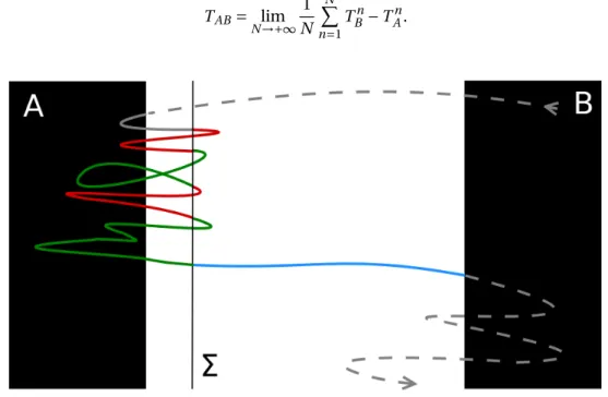
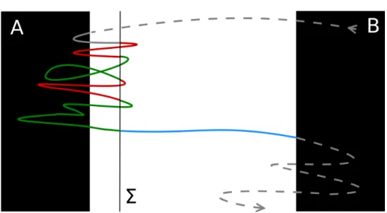
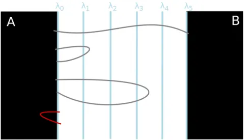
Considérons une trajectoire à l’équilibre. Par ergodicité, les deux états A et B sont visités infiniment souvent. Considérons les premières entrées successives dans l’un de ces états, après avoir visité l’autre (voir les points rouges sur la figure 1). Nous appelons (T_An)_n≥0les temps pour lesquels l’entrée est dans

A, et (T_Bn)_n≥0dans B . Les segments entre T_Anet T_Bnsont appelés les chemins de transition de A à B . Notez que ces trajectoires contiennent un chemin qui relie l’état A à l’état B sans repasser par A (en bleu sur la figure 1), appelé trajectoire réactive. La durée moyenne des trajectoires de transition à

(12)

ix

Figure 1 – Fragment de trajectoire d’équilibre. Le segment bleu correspond à une trajectoire réactive entre les

états A et B . Le temps de transition est la durée moyenne des trajectoires comme celle représentée par la ligne continue.

l’équilibre est appelée le temps de transition[8,9]. Le temps de transition est alors défini comme suit :

TAB= lim N →+∞ 1 N N X n=1 T_Bn− TAn.

Figure 2 – Décomposition de la trajectoire de transition à l’aide d’une région intermédiaireΣ proche de A, afin

de calculer le temps de transition via la probabilité de transition à partir deΣ en équilibre.

On peut calculer le temps de transition en utilisant la probabilité de transition à partir d’une région intermédiaireΣ dans le voisinage de A. Pour cela, le chemin de transition est divisé en morceaux à chaque fois qu’il traverseΣ, si A a été visité entre temps (voir figure 2). Chaque fois que la particule croiseΣ, il y a deux événements possibles : revenir dans A ou atteindre B. C’est une loi de Bernoulli,

(13)

x

et si on appelle p la probabilité à l’équilibre d’atteindre B à partir deΣ, le système reviendra dans

A un nombre 1/p − 1 de fois avant d’atteindre B. Appelons E¡Tloop¢ le temps moyen à l’équilibre de

ces allers-retours dans A, en passant parΣ. Le temps total passé à faire ces boucles, de A à Σ puis retour dans A, avant une transition peut être estimé par (1/p − 1)E¡Tloop¢. Si on noteE(Treac) la durée

moyenne de la trajectoire réactive à l’équilibre, le temps de transition peut donc être calculé comme : E(TAB) =

µ 1

p− 1

¶

E¡Tloop¢ + E(Treac) . (3)

Notez que Σ peut être choisi comme bordure de A, ce qui ne change pas l’équation ci-dessus. L’équation (3) est utilisée pour calculer le temps de transition dans la méthode AMS utilisée dans cette thèse (voir [10] et chapitre 3).

La probabilité de transition p de l’équation (3) est typiquement très petite, car il est rare d’observer une transition de A vers B . Ces événements sont, par définition, très difficiles à simuler par des méthodes de Monte Carlo en force brute, car leur observation nécessite de nombreux essais indépendants. Au cours des trente dernières années, une série de méthodes ont été spécialement développées pour simuler les transitions entre états métastables. On peut les diviser en deux familles : les méthodes biaisées et les méthodes non biaisées. La première famille est composée de méthodes où la dynamique est biaisée afin de pousser le système hors de l’état métastable plus rapidement, typiquement pour calculer des quantités thermodynamiques. Cela inclut des méthodes comme adaptive biased molecular dynamics (ABMD)[11], et les méthodes d’énergie libre, telles la méthode adaptive biasing force (ABF)[12]. La deuxième famille vise à obtenir des informations cinétiques sur la transition, en échantillonnant des trajectoires réactives. La dynamique n’est pas biaisée et d’autres stratégies sont utilisées afin de réduire le coût de calcul. Cela inclut des méthodes comme transition path sampling (TPS)[13] et ses dérivées,

transition interface sampling (TIS) et replica exchange TIS (RETIS)[14], et des méthodes de splitting, avec forward flux sampling (FFS)[15] adaptive multilevel splitting AMS, la méthode étudiée dans ce travail.

Dans les méthodes de splitting, on introduit des interfaces intermédiaires entre A et B à l’aide d’une fonction qui calcule le progrès vers B , appelée coordonnée de réaction. La stratégie consiste à simuler des chemins qui relient deux interfaces successives. La probabilité finale de transition est calculée comme un produit des probabilités de passer de chaque interface à la suivante.

Dans FFS, les interfaces qui divisent l’espace sont fixées. Mentionnons qu’il existe une version adap-tative de l’algorithme où leurs positions sont établies après quelques passes FFS, afin de minimiser la variance de l’estimateur de la probabilité p[16]. Dans AMS les interfaces sont définies de façon adaptative, au cours de l’algorithme[17].

Dans l’algorithme AMS, à chaque trajectoire est associée un niveau, qui est la valeur maximale de la coordonnée de réaction atteinte le long de la trajectoire. A chaque itération, le niveau de la kème trajectoire, appelé niveau d’élimination, définit une nouvelle interface. Toutes les trajectoires de niveau égal ou inférieur au niveau d’élimination sont tuées, et remplacées par des trajectoires choisies au hasard parmi les vivantes qui seront répliquées. La réplication consiste à copier la trajectoire jusqu’au premier point qui va plus loin que le niveau d’élimination, et à exécuter la dynamique indépendamment à partir de ce point jusqu’à atteindre A ou B (voir figure 3). Une description plus détaillée de l’algorithme est donnée au chapitre 2. Cette façon de positionner les interfaces optimise la

(14)

xi

Figure 3 – Première itération AMS avec N = 5 et k = 2. Les deux répliques de niveau inférieur (en gris) sont tuées.

Deux des répliques restantes sont sélectionnées au hasard pour être copiées jusqu’au niveau z_{ki l l}0 (ligne rouge pointillée) et ensuite continuées jusqu’à atteindre A (généralement plus probable) ou B .

variance de l’estimateur de la probabilité p. Cela fait d’AMS une méthode avec très peu de paramètres définis par l’utilisateur, qui est de plus robuste et facile à utiliser. Une preuve mathématique du caractère non-biaisé de l’estimateur de la probabilité quels que soient les paramètres de l’algorithme, qui sont le nombre total de trajectoires N , k et la coordonnée de réaction, peut être trouvée dans [18]. L’objectif de ce travail est d’étudier l’application de la méthode adaptive multilevel splitting (AMS) pour l’échantillonnage des trajectoires réactives et l’estimation des temps de transition en dynamique moléculaire. Divers systèmes ont été utilisés, et ceux-ci peuvent être divisés en deux familles. La pre-mière famille contient des modèles jouets qui ont été utilisés pour des développements méthodologiques. La deuxième famille contient des systèmes moléculaires plus complexes qui ont été étudiés grâce à la méthode AMS.

309.5 ns

φ ψ

Figure 4 – Les deux conformations stables de la molécule dipeptide alanine et les angles dièdresφ et ψ utilisés

pour les distinguer.

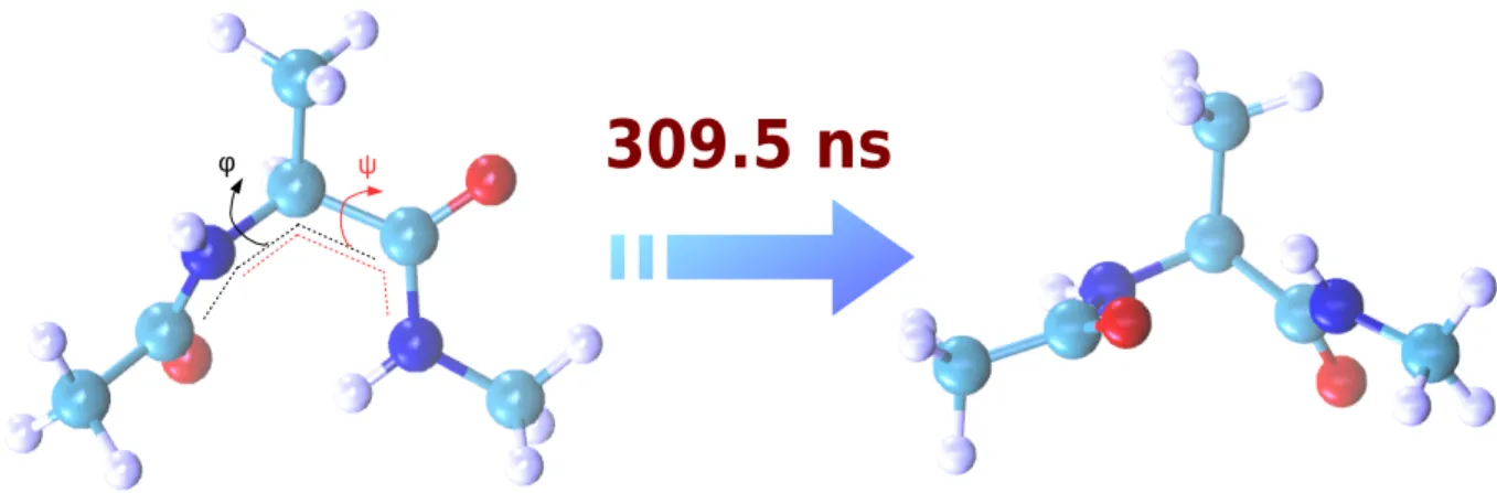
Le premier système étudié est un modèle de jouet couramment étudié, le dipeptide alanine. Cette molécule est petite et présente deux conformations stables dans le vide. En raison de sa similarité avec les peptides, qui jouent un rôle important dans le repliement des protéines, l’un des processus les plus difficiles à simuler, ce modèle est devenu un système couramment utilisé pour tester de nouvelles

(15)

xii

méthodes pour l’analyse des systèmes biomoléculaires. La figure 4 montre les deux conformations du dipeptide alanine, facilement décrites par deux angles dièdres.

L’étude des changements conformationnels de cette molécule permet tout d’abord de valider l’AMS par rapport aux résultats de référence obtenus par simulation directe, et démontre la robustesse des résultats AMS, notamment en ce qui concerne le choix de la coordonnée de la réaction. De plus, nous proposons un nouveau protocole pour échantillonner correctement la condition initiale lors de l’utilisation de l’AMS pour obtenir le temps de transition. Nous expliquons également comment estimer deux quantités intéressantes en utilisant les trajectoires générées par l’AMS afin d’explorer les chemins de réaction. Le premier est le flux des trajectoires réactives, et le second est la fonction committor. Les résultats de cette étude ont été publiés dans le Journal of Computational Chemistry[19]. Deux questions soulevées au cours de ce projet ont conduit aux études suivantes de la première partie de la thèse. La première concerne l’échantillonnage des conditions initiales dans AMS pour calculer le temps de transition. Nous proposons une nouvelle technique combinant AMS et un échantillonnage par fonction d’importance, présentée au chapitre 3. La seconde porte sur l’utilisation des trajectoires réactives générées par l’AMS pour élucider les mécanismes de réaction en s’appuyant sur des techniques de clustering, présentées au chapitre 4.

Pour comprendre la source du problème d’échantillonnage des conditions initiales, nous étudions les transitions sur le potentiel unidimensionnel V (x) = x4− 2x2, qui présente deux états métasta-bles, autour de x = −1 et x = +1. Ce même problème jouet a également été étudié par T. van Erp dans [14], où les méthodes FFS et RETIS ont été appliquées. Dans [14], les résultats obtenus par FFS ne coïncident pas avec les résultats de référence. Tout d’abord, nous effectuons la même expéri-ence numérique que dans [14] en utilisant AMS, et montrons que, malgré l’apparente simplicité du problème, l’échantillonnage des conditions initiales en utilisant AMS, et donc aussi FFS, est crucial pour obtenir des résultats cohérents. Nous expliquons et proposons donc une solution aux obser-vations numériques de [14]. Nous proposons ensuite une nouvelle technique, combinant AMS et l’échantillonnage par fonction d’importance, pour échantillonner plus efficacement les conditions ini-tiales, que nous validons sur ce cas unidimensionnel. Nous discutons également comment appliquer cette technique à des cas multidimensionnels.

Pour élucider les mécanismes de réaction, nous proposons une nouvelle façon de les extraire, en effectuant un clustering sur l’ensemble des trajectoires réactives obtenues avec AMS. L’obtention du mécanisme de transition est un vieux problème. La littérature sur le sujet ne donne pas une défini-tion claire d’un mécanisme de transidéfini-tion, voir [20–23]. En outre, beaucoup des travaux précédents supposent qu’il n’existe qu’un seul mécanisme possible, ce qui n’est pas toujours le cas pour des systèmes complexes. La méthode des tubes de transition, introduite par Vanden-Eijnden dans [9], a été la première à considérer plus d’un mécanisme, cependant ces tubes ne sont pas définis de façon unique. En effectuant un clustering des trajectoires réactives, les trajectoires représentatives de chaque cluster peuvent être considérées comme des mécanismes de réaction possibles. De plus, la technique de clustering permet non seulement l’existence de plus d’un mécanisme, mais donne également une probabilité à chacun d’entre eux. Nous présentons dans ce manuscrit les résultats préliminaires obtenus avec deux systèmes. Le premier est un potentiel bicanal en dimension deux, où la température influence le trajet privilégié, ce qui se traduit par une différence de poids des clusters. Le second est le dipeptide alanine à partir de différentes conditions initiales, où le nombre de mécanismes n’est

(16)

xiii pas connu à priori. Cette étude a été réalisée en collaboration avec Jacques Printems, de l’Université Paris-Est Créteil.

Dans la deuxième partie de la thèse, nous présentons sur trois chapitres des études sur NAMD utilisant AMS. Dans cette thèse, l’implémentation de la méthode AMS pour NAMD dans Tcl a été améliorée, et un ensemble de scripts bash a été écrit afin de fournir un moyen plus facile d’utiliser cette méthode. On peut définir des simulations AMS en fournissant un simple fichier de configuration et quelques scripts pour définir les paramètres de l’algorithme, y compris les coordonnées de la réaction. Afin de diffuser la méthode au sein de la communauté NAMD, un tutoriel basé sur le changement conformationnel de la molécule dipeptide alanine a été rédigé. Ce tutoriel est publié sur la page web des tutoriels NAMD, qui fournit également tous les fichiers nécessaires pour compléter le tutoriel. Le chapitre 5 présente le tutoriel publié.

ligand I

ligand II

Figure 5 –β-cyclodextrine avec les ligands I et II, et deux images d’une trajectoire de sortie générée avec AMS. Le

ligand I sort par le bas, toujours en contact avec laβ-cyclodextrine. Le ligand II sort par le haut, et son contact se

fait par son groupe hydroxyle. Nos résultats ont montré que les contacts entre le ligand et le piège ont un rôle important dans le mécanisme de déblocage.

Les cyclodextrines sont une famille de molécules formées par des unités répétées de glucopyranose, générant une structure cyclique avec un intérieur hydrophobe et un extérieur hydrophile. Ainsi, les cyclodextrines ont la capacité d’augmenter la solubilité des molécules hydrophobes dans l’eau, et sont donc utiles dans de nombreuses applications industrielles[24]. Dans cette thèse, nous simulons la sortie de deux ligands différents de l’intérieur de laβ-cyclodextrine vers un environnement aqueux.

(17)

xiv

Nous montrons que les calculs AMS donnent un résultat fiable, avec un coût de calcul divisé par 400 lorsque la comparaison avec des simulations numériques directes est possible.

Puisque les ligands restent piégés à l’intérieur de laβ-cyclodextrine à cause de son intérieur hy-drophobe, il est clair que l’eau joue un rôle important dans la sortie du ligand. C’est une propriété que l’on retrouve également dans d’autres processus de sortie des molécules cages. Nous comparons deux modèles d’eau couramment utilisés dans les systèmes biomoléculaires : TIP3P et TIP4P/2005[25,26]. Nos résultats ne montrent pas de différence significative dans le mécanisme de sortie, ce qui signifie que le passage de TIP3P à TIP4P/2005, un modèle plus coûteux sur le plan informatique, ne modifie pas de manière qualitative le comportement décrit des molécules. Toutefois, une différence significative est observée en ce qui concerne le temps de sortie. Cette différence s’explique par des variations des coefficients de diffusion et, dans une moindre mesure, par la durée de vie variable des liaisons hydrogènes entre le ligand et laβ-cyclodextrine. Il est également important de mentionner qu’il nous reste encore à explorer d’autres effets pour expliquer entièrement la différence observée, tels que l’énergie de solvatation des ligands dans l’eau. Les résultats de ce projet sont présentés dans le chapitre 6.

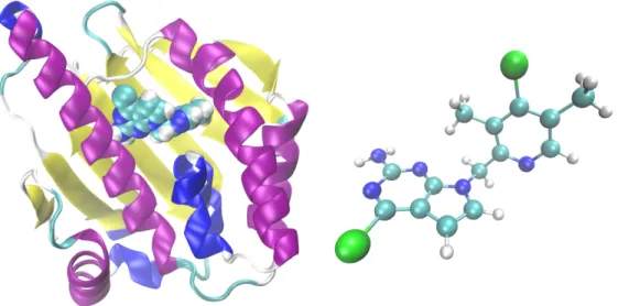
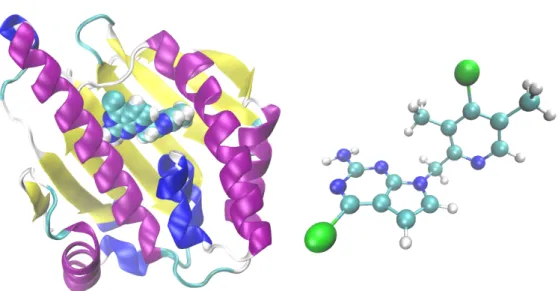
Le dernier système étudié est la protéine heat shock 90 (Hsp90), qui est une protéine chaperonne humaine surexprimée dans certains types de cancer, rendant ces cellules cancéreuses plus sensibles aux médicaments qui bloquent l’activité de la Hsp90. Une cible typique de cette protéine est son domaine N-terminal, qui se lie à l’ATP pour alimenter le cycle fonctionnel de la protéine. Étant donné que l’efficacité du médicament dépend de son temps de séjour dans le lieu de liaison, il est important d’obtenir une estimation du temps de détachement lorsque l’on cherche un nouveau médicament. Nous appliquons la méthode AMS pour simuler le détachement d’un ligand du domaine N-terminal du Hsp90, cf. le chapitre 7. Ce projet est réalisé en collaboration avec des chercheurs de l’entreprise pharmaceutique Sanofi.

Figure 6 – N-terminale de Hsp90, avec un ligand à l’intérieur de sa cavité (structure PDB 5LR1), et la molécule

de ligand (A003498614A).

(18)

xv par Sanofi, puis publiée sous le nom de Protein Data Bank id 5LR1 (voir figure 6). La structure peu commune du ligand nécessite un paramétrage du champ de force basé sur un terme croisé CMAP, où la molécule a été divisée en deux fragments pour permettre le calcul des constantes de force de liaison et d’angle, ainsi que des charges.

La détermination de l’état métastable lié a été faite en utilisant une première simulation suivant la dynamique libre, à partir de la structure cristallographique. De plus, des simulations ABMD ont été utilisées pour explorer d’autres états métastables possibles, liés ou intermédiaires. Cette approche s’est révélée incomplète et c’est avec l’AMS que deux autres états liés ont été découverts.

En utilisant les résultats AMS, et avec des calculs d’énergie libre, nous avons pu déterminer la nature des nouveaux états trouvés, et proposer une nouvelle coordonnée de réaction et une nouvelle définition pour l’état lié. Les simulations utilisant ces nouveaux paramètres sont en cours d’exécution, et quatre trajectoires réactives ont été générées jusqu’à présent. Toutes les simulations ont été réalisées avec les ressources HPC de GENCI [Occigen].

En résumé, ce travail de thèse a permis d’améliorer l’utilisation de la méthode AMS pour étudier les transitions entre états métastables pour des systèmes dynamiques stochastiques utilisés en dy-namique moléculaire. Le travail méthodologique a notamment porté sur l’échantillonnage correct des conditions initiales. De plus, l’implémentation de la méthode dans NAMD a été améliorée, ce qui a permis de nouveaux tests sur des systèmes biologiques d’intérêt pour des applications industrielles.

(19)

(20)

5.1 The Adaptive Multilevel Splitting method . . . 78 5.1.1 The AMS algorithm . . . 79 5.1.2 Setting up AMS simulations . . . 81 5.2 Applying AMS to the alanine dipeptide isomerization in vacuum . . . 83 5.2.1 Definitions of A, B andξ . . . 84 5.2.2 Calculating the probability with AMS . . . 85 5.2.3 Obtaining the transition time using AMS results . . . 87 5.2.4 Calculating the flux of reactive trajectories sampled with AMS . . . 89

6 β-Cyclodextrin-ligand unbinding mechanism and kinetics: influence of the water model 91 6.1 Introduction . . . 91 6.2 Methods . . . 93 6.2.1 The Adaptive Multilevel Splitting Method for ligand unbinding fromβ-cyclodextrin 95 6.2.2 The Transition Time Equation . . . 97 6.3 Results . . . 98 6.3.1 Unbinding mechanism . . . 100 6.3.2 Understanding the difference in kinetics between the water models . . . 103 6.4 Conclusion and Perspectives . . . 104

7 Ligand unbinding from Heat Shock Protein 90 107

7.1 Introduction . . . 107 7.2 Set up of the system and numerical method . . . 108 7.2.1 Custom force field for the ligand . . . 108 7.2.2 Calculating the unbinding time with AMS . . . 111 7.3 Details on the numerical procedures and results . . . 113 7.3.1 First AMS results . . . 116 7.3.2 Analyzing metastable states to prepare new AMS simulations . . . 117 7.4 Conclusion and Perspectives . . . 119

(23)

(24)

Chapter 1 Introduction

The objective of this work is to study the application of the adaptive multilevel splitting (AMS) method to the sampling of reactive trajectories and the estimation of transition times in molecular dynamics. A range of systems were used, which can be separated into two groups. The first one contains simple models that allowed us to propose improvements to the AMS method in general. The second one contains more realistic and challenging systems, where AMS is used to advance our understanding on the molecular mechanisms.

This chapter presents the framework of the thesis. The reader will find a description of molecular dynamics, force fields and a review of different methods to simulate rare events in molecular dynamics. Next, a summary of the main contributions, including a brief description of the encountered problems and the obtained results is presented.

1.1 Molecular Dynamics

Molecular Dynamics is the name given to the numerical method used to simulate molecules in vacuum or in solvent, assuming that the nuclei envolve following classical Newtonian dynamics plus possibly some terms to model the chosen thermodynamical ensemble. Introduced by Alder and Wainwright in the 50’s, the goal was originally to describe and understand intrinsically multibody effects, like phase transitions[1], describing molecules as rigid spheres. The method became quickly popular among theoretical chemists and physicists and the first studies of liquids at a molecular level appeared in the literature in the 70’s[2]. The raising interest in describing the behavior of large scale systems, for which the quantum approaches are still impossible, pushed the development of the model. In the last five decades, a range of molecular dynamics programs and classical potentials, called force fields, have been developed.

1.1.1 Langevin Dynamics

Langevin dynamics is typically used to describe the movement of atoms at a fixed temperature. This dynamics modifies deterministic Hamiltonian dynamics, which preserves energy, with stochastic

(25)

2

terms, which model the fluctuations of the system due to temperature. Let us call (qt, pt) the positions and momenta at time t of the particles inR6N, where N is the number of atoms. Langevin dynamics models the evolution of (qt, pt) as follows:

(

d qt = M−1ptd t ,

d pt = −∇V (qt)d t − γM−1ptd t +p2γβ−1dWt.

(1.1)

In the equation above, V denotes the potential function, also called force field, M is the mass tensor and

γ is the friction parameter. The process Wtis a Brownian motion in dimension 3N . The multiplicative term in front of Wtdepends on the temperature via the parameterβ−1_{= kB}_{T .}

It is important to mention that, for a molecular system, the timestep of any numerical solution of Langevin dynamics is bounded from above. This is due to the natural oscillations caused by the covalent bonds, whose typical periods sets a maximum value for the timestep, such that the numerical solution is capable of simulating them accurately. The higher frequency oscillations are those of covalent bonds with hydrogen atoms. A C-H bond stretch in alkanes has a typical period around 10 femtosecond. This gives an upper bound on the timestep of the order of 1 fs. A typical strategy to raise the timestep is to fix all the lengths of the covalent bonds involving hydrogen atoms in the system, enabling a timestep of 2 fs[27].

1.1.2 Force Fields

Force field is the given name for the classical empirical potential V of the molecular system. This function includes two types of terms: those that try to carry a physical sense to the interactions; and those added when the latter terms alone are not able to predict the correct behavior of the molecule, and which have no clear physical interpretation. The first terms include the bonded terms, which describe the interactions between two to four bonded atoms, and depend on bond lengths, angles and dihedral angles; and the non-bonded terms, which describe the interactions between atoms which are not covalently bonded, in the same molecule or not, through a Coulomb and a Lennard-Jones potential. When the latter terms are not sufficient to reproduce the correct behavior of the molecule, other terms are added. For example, the improper term is a harmonic potential over a dihedral between non-bonded atoms. Functions that depends on two internal variables, called cross terms, can be used to model interactions between these internal degrees of freedom.

The chosen force field fixes the functional forms of the terms used to model the interactions. Once the functional form is chosen, the functions’ parameters are empirically determined, through a fit over experimental or ab initio data. For example, for the CHARMM force field[3], the most common terms in the potential are given by:

VCHARMM = X bonds K_{i j}b ³bi j− b0_{i j} ´2 +X angles K_{i j k}θ ³θi j k− θ0_{i j k} ´2 + X dihedrals K_{i j kl}ϕ £1 + cos ¡nϕi j kl− δ¢¤ + X nonbonded pairs qiqj ²ri j + εi j   Ã_r0 i j ri j !12 − 2 Ã_r0 i j ri j !6 + X impropers K_{i j}ω³ωi j− ω0i j ´2 . (1.2)

(26)

3 For some types of molecules, which have common atom types and environments, generic parameters can be found. This is typically the case for proteins, where force fields like AMBER and CHARMM are well validated to describe their behavior[3,4]. But this is only possible because proteins are composed of a small variety of repetitive units. For a few molecules studied in this thesis a specific, and thus non-transferable, force field was parameterized. It is important to mention that, because of the large number of parameters to be determined, the optimization problem is not easy to solve. There is a well established protocol to parameterize force fields by determining the most well-determined and important parameters first.

In this thesis, the CHARMM force field was used and the parameterizations were done with the help of the force field toolkit (FFTK) from VMD[5,6], whose aim is to determine optimal parameters with respect to ab initio computations. When fitting a force field to ab initio data, the first step is to obtain the lowest energy positions of the nuclei, namely the optimized geometry. This will give the equilibrium values for the internal variables. The first goal of a force field is indeed to correctly describe the equilibrium conformation. The bonds and angles are described by a harmonic potential, which requires to compute the Hessian matrix for the system in order to obtain the force constants. The last parameters are the charges and the parameters related to the dihedrals angles, that are less direct and harder to determine.

Because charges are introduced to model the intermolecular interactions, they are primarily fitted to correctly describe the strongest bond between two molecules, which is the hydrogen bond with a water molecule. Thus, next to every donor and acceptor atom, a water molecule is placed and its distance and orientation are optimized with a quantum calculation. Using this data, and starting from a first guess that is given by the user, the charges are optimized, generally using a simulated annealing algorithm. Because all charges are fitted at the same time, this consists in a high dimension optimization. Hence, the convergion to the global minimum is difficult and spurious phenomena can appear. To avoid them additional contrains may be added. In Chapter 7 this was made by fitting the charges to fragments of the molecule separetly, which required additional ab initio data.

The torsion parameters, associated with the dihedral angles, are determined by fitting the result of an ab initio relaxed energy scan. This means that, for a range of values around the equilibrium, the dihedral angle is fixed and the geometry is optimized. The result is the energy as a function of the dihedral angles, which is then fitted using a periodic cosine function. Despite the apparent simplicity of this step, it is in this last stage that the necessity to use improper or cross terms is discovered. For example, in the parameterization presented in Chapter 7, a cross term was needed to describe the energy variation caused by two dihedral angles that had three atoms in common, and thus were correlated and could not be computed as a sum of two terms. For that case we used a CMAP correction, which is a grid based energy correction function of two dihedral angles, firstly introduced in 2004 to better describe protein backbones in CHARMM[28].

Another particularity of the force field parameterized in Chapter 7 was the use of two fragments of the molecule to calculate the bond, angle and charge parameters. This was necessary because the molecule was too large to compute the full Hessian. These fragments were again used when the charge optimization revealed a spurious dipole in the molecule, which was corrected by fitting the charges to both fragments separately.

(27)

4

to mention that classical force fields are currently the cheapest way to calculate the energy of the system, and thus enable the calculation of the classical dynamics of large systems using the current computational resources. Notice that, during the dynamics, the forces of the system need to be computed at every timestep, which in molecular dynamics is limited by a maximum of 2 fs. For different problems one can use more elaborated force fields, including polarization effects or even the possibility of a chemical reaction, which imply of course a larger computational cost.

1.1.3 The NAMD molecular dynamics software

All the molecular simulations in this thesis were performed using the NAMD program[7]. NAMD is a molecular dynamics program that has a good scalability and is thus appropriate to simulate large scale systems on different architectures. For this reason, it is widely used by the biophysics community. The implementation of the AMS method in NAMD was initiated by C. Mayne and I. Teo in [29], and was pursued in the framework of this PhD thesis (see Chapter 5). The AMS method was implemented in Tcl, the language used by NAMD to parse the configuration file. It is therefore easy to implement a new method for this program. It is also important to mention that the AMS method requires the definition of a progress function, called a reaction coordinate, that depends on internal variables of the system. The Colvars plugin for NAMD/VMD[30], which has Jérôme Hénin as one of its developers, was used to easily obtain the collective variables to compute the reaction coordinate.

1.1.4 Metastable states and their transitions

Metastable states are defined as regions where the system stays trapped for a considerable amount of time. Hence, transitions between two metastable states, or the escape from one, are rare events. Examples of rare events in our everyday life includes earthquakes or major floods. In chemistry, protein folding, ligand unbinding from a protein cavity and opening or closing of channels in cell membranes are examples of rare events.

Rare events are, by definition, very difficult to simulate by brute force Monte Carlo methods, since observing them requires many independent trials. Over the past thirty years, a range of methods were specially developed to simulate transitions between metastable states. They can be divided into two families: biased and non-biased methods. The first family consists in methods where the dynamics is biased in order to push the system out of the metastable state faster, typically to compute thermodynamic quantities. This includes adiabatic bias molecular dynamics (ABMD)[11], and free energy methods, such as adaptive biasing force[12]. The second family aims at obtaining kinetic information about the transition. The dynamics is not biased and other strategies are used in order to shorten the computational cost. AMS, which is the method studied in this work, belongs to this second family.

(28)

5

1.2 Methods for the simulation of reactive paths

In this thesis, we will focus on unbiased methods to obtain kinetic information about reactive paths. The goal is in particular to obtain the transition time, or its inverse, the transition rate. Let us call A a metastable region from which we want to simulate escapes, and B a target state. Let us consider a system with N atoms, so the dynamics is overR6N(position and momentum for all particles). This means that A and B are subsets ofR6N. In chemistry, those states are defined using a small set of internal variables, that in practice actually only depends on the positions of the particles.

The reader will find a brief discussion about transition path theory, including the definition we will use for transition time and reaction rate, in section 1.2.1. Then we discuss different equations used to calculate the transition time and the transition rate in section 1.2.2. Next we present a summary of methods commonly used in molecular dynamics to simulate transition paths. Section 1.2.3 focus on transition path sampling and its derivatives, and section 1.2.4 on splitting methods.

1.2.1 Transition Path Theory

Figure 1.1 – Fragment of an equilibrium trajectory. The blue segment corresponds to a reactive trajectory

between states A and B . The transition time is the average duration of trajectories like the one represented by the solid line.

Let us consider a trajectory at equilibrium. By ergodicity, the two states A and B are visited infinitely many times. Let us consider the successive first entrances in one of those states, after having visited the other one (see the red dots on figure 1.1). We call (T_An)_n≥0the times for which the entrance is in A, and (T_Bn)_n≥0in B . The segments between T_Anand T_Bnare called the transition paths from A to B . Notice that those trajectories contain a path that links state A to state B (in blue on figure 1.1), called the reactive trajectory. The average duration of the transition paths at equilibrium is called the transition

(29)

6

time[8,9]. The transition time is then defined as:

TAB= lim N →+∞ 1 N N X n=1 T_Bn− TAn.

It is also common to define the transition rate, which is the inverse of the transition time:

kAB= 1

TAB .

The transition path theory gives formulas for these quantities using the committor function, which for each point in space measures the probability to reach B before A starting from that point, see for example Proposition 1.8 in [8].

1.2.2 Computing the transition time

Figure 1.2 – Decomposition of the transition path using an intermediate regionΣ near A, in order to calculate

the transition time via the probability of transition starting fromΣ at equilibrium.

One can calculate the transition time using the probability of transition starting from an intermediate regionΣ in the neighborhood of A. For that, the transition path is splitted into pieces at every time it crossesΣ, if A was visited just before (see figure 1.2). Whenever the particle crosses Σ there are two possible events: going back to A or reaching B . This is a Bernoulli law, and if we call p the probability at equilibrium to reach B starting fromΣ, the system will go back to A a number 1/p −1 of times before reaching B . Let us callE¡Tloop¢ the average time of those returns to A at equilibrium, passing through

Σ. The total time spent doing loops, from A to Σ and back to A, before a transition can be computed as (1/p −1)E¡Tloop¢. CallingE(Treac) the average reactive trajectory duration at equilibrium, the transition

time can thus be computed as:

E(TAB) = µ 1

p− 1

¶

(30)

7 Notice thatΣ can be chosen as the border of A, which does not change the equation above.

Equation (1.3) is used to compute the transition time in the AMS method (see [10] and Chapter 3). Other rare event methods[15] use the following equation to obtain the transition rate:

kAB=

p

E¡Tloop¢ .

(1.4) Notice that, if the probability p is small, the second term of equation (1.3) is negligible compared to the first. Hence, equation (1.4) is equivalent to equation (1.3) in this regime.

Another common way to compute the transition rate is via the correlation function C (t ), which measures the probability to be inside B at time t , if the particle was inside A at the initial time. Let us introduce the function hA(resp. hB) that is unity inside A (resp. B ) and zero elsewhere. The correlation function C (t ) is defined as:

C (t ) =〈hA(x0)hB(xt)〉

〈hA(x0)〉

, (1.5)

where xtis the position of all the particles in the system at time t . This function is linear in short time, and the linear constant is the reaction rate, i.e. C (t ) ≈ kABt [15].

1.2.3 Transition Path Sampling

Transition path sampling (TPS) is a method introduced in the 90’s [13], were the reactive trajectories are sampled directly in the path space using a Metropolis Monte Carlo algorithm. A first reactive trajectory is generated and a new one is obtained from the first in a trial move. The new trajectory have a probability of acceptance that is nonzero only if it is also reactive. There are various versions of the algorithm, which differ in the kernel to propose new trajectories, the calculation of the acceptance probability, and the calculation of the transition rate.

Figure 1.3 – The shooting move used to generate new trajectories in TPS and its derivatives. The gray trajectory

is the old one. From the shooting point (red dot) the momentum of the atoms is changed and the dynamics is run forward and backward for the same number of timesteps. In other versions the new segments are run until it reaches A or B , in order to allow the trajectory duration to vary.

(31)

8

In the original version of TPS, new trajectories are generated through the so-called shooting move, starting from a randomly chosen point of an existing trajectory of fixed sizeτ. Let us call (x_to)_{t ∈[0,τ]}the first trajectory, and xo_t0the chosen point, called the shooting point. A perturbation in the momentum of the atoms is done, generating a new point xn_t0, from where the dynamics is run both forward and backward, in order to complete the new path of equal sizeτ, (xn_t)_{t ∈[0,τ]}. The probability to accept this trial move is only nonzero if the new trajectory is reactive, and depends on the density of the first points of both trajectories. If the initial conditions are at equilibrium and the probability to generate the shooting point is symmetric, in the sense that it is equaly probable to obtain xn_t0from x_to0 that to obtain xo_t0from x_tn0, then the acceptance probability is given by[13]:

Pacc(o → n) = hA¡x0n¢ hB¡xτn¢ min " 1,ρ ¡x n 0 ¢ ρ ¡xo 0 ¢ # .

The final transition rate is calculated using the correlation function from equation (1.5).

Figure 1.4 – Space between A and B split using five interfaces, and a few trajectories. The first trajectory is

reactive. The second crossesλ1, so it belongs to the path ensemble [1+]. The third goes further, and hence

belongs to [3+]. The red trajectory is only considered in RETIS, and belongs to the path ensemble [0−].

A variation of the TPS method, called transition interface sampling (TIS), was later developed, in which the rate constant is calculated using the transition probability via equation (1.4)[14]. Using isolevel surfaces of an order parameterλ : R6N→ R, the space between states A and B is split. The state A is defined as {x,λ < λ0}, and a last interface n defines state B as {x,λ > λn}. The probability p in equation

(1.3) is obtained as the product of the conditional probabilities to reach one interface starting from the previous one, as:

p =

n−1 Y i =0

P(λi→ λi +1) .

The interfaces also defines the path ensembles [i+], that contains all the trajectories that crosses the interfaceλi.

The trajectories in TIS are generated by performing either a time reversal move or a shooting move. In the first move, a new trajectory is generated by changing the time direction of the original path.

(32)

9 The second move is similar to the one performed in TPS, but the duration of the trajectories vary. Starting from the shooting point, the segments are run forward and backward in time until A or B is reached. Differently from TPS, the acceptance probability is nonzero if the new trajectory starts in A and crosses either the same or a further interface than the original trajectory. This means that if the original trajectory belongs to [i+], the new trajectory must at least be in the same path ensemble. The replica exchange transition interface sampling (RETIS) is a variation of TIS where the trajectories are generated in the same way, but additional swapping moves are performed between the path ensembles[14]. Those decrease the correlation between the trajectories in the same ensemble, leading to a more efficient algorithm. An additional ensemble [0−] is also considered, which contains the trajectories that explore state A, i.e. cross interfaceλ0but in the direction of state A.

1.2.4 Splitting methods

In splitting methods, one introduces intermediate interfaces between A and B , as in TIS, but the way the trajectories are sampled is different. The strategy is to simulate paths that link two successive interfaces. The final transition probability is again calculated as a product of the probability to pass from each interface to the next one.

Forward flux sampling (FFS) is a commonly used splitting method[15]. All the points that crosses the interfaces are kept, and are then used to generate new attempts to observe trajectories that reaches the next interface. These attempts are also used to compute the probability between the interfaces. In FFS, the interfaces that split the space are fixed as level sets of a chosen scalar valued order parameter (a.k.a. reaction coordinate). Let us mention that there exists an adaptive version of the algorithm were their positions are set after a few FFS runs, in order to minimize the variance of the probability estimator[16].

Figure 1.5 – First AMS iteration with N = 5 and k = 2. Both lower level replicas (in gray) are killed. Two of the

remaining replicas are randomly selected to be copied up to level z0_{ki l l}(dotted red line) and then continued until they reach A (typically more likely) or B .

In the adaptive multilevel splitting (AMS) method, the interfaces are set on the fly[17]. Each trajectory is associated with a level, which is the maximum reached value of the reaction coordinate along the trajectory. At each iteration, the kthtrajectory level, called the killing level, defines a new interface. All the trajectories with equal or lower level are killed, and replaced by randomly chosen and replicated

(33)

10

trajectories among the living ones. The replication consists in copying the trajectory until the first point that went further than the killing level, and running the dynamics independently from that point until A or B is reached (see figure 1.5). A more detailed description of the algorithm is given in Chapter 2.

This way of positioning the interfaces optimizes the variance of the estimator. This also makes AMS a method with very few user defined parameters, which is thus more robust and easy to use. A mathe-matical proof of the unbiasedness of the probability estimator whatever the algorithm parameters, which are the total number of trajectories, k and the order parameter, can be found in [18].

1.3 Outline of this manuscript

In this thesis, two kinds of studies were done, and for this reason the chapters are organized in two parts. Part I contains the methodological results, which rely on simulations on toy models and includes chapters 2, 3 and 4. Chapter 2 contains the first study, done using a simple biomolecule. Two questions raised during that project led to the next chapters of Part I. The first one concerns the sampling of the initial conditions in AMS to compute the transition time. We propose a new technique combining AMS and importance sampling, presented in Chapter 3. The second one is about using the reactive trajectories generated with AMS to elucidate reaction mechanisms, for which we propose clustering techniques, presented in Chapter 4. Part II contains numerical results on more complicated molecular systems studied thanks to the AMS method, and includes chapters 5, 6 and 7. Chapter 5 contains the tutorial of the AMS implementation on NAMD. Chapter 6 presents the study of the influence of the water model in theβ-cyclodextrin and ligand unbinding process. Chapter 7 contains the application of the AMS method to sample unbinding trajectories of a ligand from a protein cavity. In the following sections, we present a brief summary of each of these projects.

It is important to mention that the chapters of this manuscript are written in a self contained form, so that the reader can find all the necessary information to understand the project in the same chapter. This implies some repetitions from one chapter to another, in particular, the description of the AMS algorithm and the formula used to compute the transition time. The most precise and complete description of those are found in chapters 2 and 3, respectively.

Chapter 2: Alanine di-peptide

The first studied system is a molecular toy model, the alanine di-peptide. This molecule is small and exhibits two stable conformations in vacuum. Because of its similarity with peptides, which has an important role in protein folding, one of the most difficult process to simulate, this model became a commonly used system to test new methods for the analysis of biomolecular systems. Figure 1.6 shows the two conformations of the alanine di-peptide, easily described by two dihedral angles. The study of the conformational changes of this molecule allows us to first validate AMS against brute force results, and demonstrates the robustness of the AMS results, in particular with respect to the choice of the reaction coordinate. Moreover, we propose a new protocol to correctly sample the initial condition when using AMS to obtain the transition time. We also explain how to estimate

(34)

11

309.5 ns

φ ψ

Figure 1.6 – The two stable conformations of the alanine di-peptide molecule and the dihedral anglesφ and ψ

used to distinguish them.

two interesting quantities using the trajectories generated by AMS in order to explore the reaction pathways. The first one is the flux of reactive trajectories, and the second one is the committor function. Results of this study were published in the Journal of Computational Chemistry[19].

Chapter 3: 1D potential

In Chapter 3, we study transitions on the one dimensional potential V (x) = x4− 2x2, which exhibits two metastable states, around x = −1 and x = +1. This was also studied by T. van Erp in [14], where the FFS and RETIS methods were applied. In [14], the results obtained by FFS do not coincide with reference results.

First we perform the same numerical experiment as in [14] using AMS, and show that, despite the apparent simplicity of the problem, the sampling of initial conditions when using AMS, and thus also FFS, is crucial to obtain consistent results. We thus explain and propose a solution to the numerical observations of [14]. We then propose a new technique, combining AMS and importance sampling, to more efficiently sample the initial conditions, which we validate on this one dimensional case. We also discuss how to apply this technique to multidimensional cases.

Chapter 4: Clustering of reactive trajectories

In this work we propose a new way to extract reaction mechanisms, by performing a clustering on the ensemble of reactive trajectories obtained with AMS. Obtaining the transition mechanism is an old problem. The literature on the subject does not provide a clear definition of a transition mechanism[20–

23]. Moreover, many of the previous works assume that there is only one possible mechanism, which is not always the case in complex systems. The transition tubes introduced by Vanden-Eijnden in [9] was the first method to consider more than one mechanism, but they are not uniquely defined. By performing a clustering of the reactive trajectories, the representative paths from each cluster can be considered as a possible reaction mechanisms. In addition, the clustering technique not only enables the existence of more than one mechanism, but also gives a weighting probability to each one.

(35)

12

Chapter 4 presents preliminary results obtained using two systems. The first one is a bi-channel potential in dimension two, where the temperature influences the preferable path, which is seen by the difference in the cluster weights. The second is the alanine di-peptide starting from different initial conditions, where the number of mechanisms vary. This study was made in collaboration with Jacques Printems, from Université Paris-Est Créteil.

Chapter 5: AMS tutorial for NAMD

In this thesis the implementation of the AMS method for NAMD in Tcl was improved, and a set of bash scripts was written in order to provide a more easy way to use the method. One can set AMS simulations providing one simple configuration file and a few scripts to set the parameters of the algorithm, including the reaction coordinate. In order to diffuse the method among the NAMD community, a tutorial based on the conformational change of the alanine dipeptide molecule was written. This tutorial is published in the NAMD tutorials webpage, that also provides all the files necessary to complete the tutorial. Chapter 5 presents the published tutorial.

Chapter 6:

β

-cyclodextrin with ligand

Cyclodextrins are a family of molecules formed by repeated glucopyranose units, generating a ring structure with a hydrophobic interior and a hydrophilic exterior. Hence, cyclodextrins have the ability of increasing the solubility of hydrophobic molecules in water, and are thus useful for many industrial applications[24]. In this thesis, we simulate the unbinding of two different ligands from the β-cyclodextrin interior to an aqueous environment. The goal of this project is thus to apply AMS to a more complex case and compare our findings with published experimental results for the ligand’s unbinding rate[31]. We show that the AMS calculations give reliable result, with a computational cost divided by 400 when comparison with direct numerical simulations is possible.

We observed some discrepancies between the results from the molecular dynamics model and the experimental results. Willing to gain more knowledge about this system, we then change the water model and explore its influence on the unbinding process.

Since the ligands stay trapped in the interior of theβ-cyclodextrin because of its hydrophobic interior, its is clear that the water plays an important role in the ligand’s escape. This is a property also seen in other unbinding processes from cage molecules, and thus the analysis of the influence of the water model is of general interest. We thus compare two commonly used water models in biomolecular systems: TIP3P and TIP4P/2005[25,26].

Our results show no significant difference in the unbinding mechanism, meaning that the change from TIP3P to TIP4P/2005, a more computationally costly model, does not interfere in the described behavior of the molecules. However, a significant difference is observed for the unbinding time. This is caused by variations of the diffusion coefficients and, to a less extent, by the varying lifetime of the H-bonds between the ligand and theβ-cyclodextrin. It is also important to mention that we still need to explore other effects to entirely explain the difference seen in the unbinding times, such as the solvation free energyof the ligands in water.