Nouvelles méthodes informatiques et statistiques pour analyser les données du criblage à haut débit

NOUVELLES MÉTHODES INFORMA TIQUES ET STATISTIQUES POUR ANAL YSER LES DONNÉES DU CRIBLAGE À HAUT DÉBIT

THÈSE PRÉSENTÉE

COMME EXIGENCE PARTIELLE DU DOCTORAT EN INFORMA TIQUE

PAR IURIE CARAUS

UNIVERSITÉ DU QUÉBEC À MONTRÉAL Service des bibliothèques

Avertissement

La diffusion de cette thèse se fait dans le respect des droits de son auteur, qui a signé le formulaire Autorisation de reproduire et de diffuser un travail de recherche de cycles supérieurs (SDU-522 - Rév.0?-2011 ). Cette autorisation stipule que «conformément à l'article 11 du Règlement no 8 des études de cycles supérieurs, [l'auteur] concède à l'Université du Québec à Montréal une licence non exclusive d'utilisation et de publication de la totalité ou d'une partie importante de [son] travail de recherche pour des fins pédagogiques et non commerciales. Plus précisément, [l'auteur] autorise l'Université du Québec à Montréal à reproduire, diffuser, prêter, distribuer ou vendre des copies de [son] travail de recherche à des fins non commerciales sur quelque support que ce soit, y compris l'Internet. Cette licence et cette autorisation n'entraînent pas une renonciation de [la] part [de l'auteur] à [ses] droits moraux ni à [ses] droits de propriété intellectuelle. Sauf entente contraire, [l'auteur] conserve la liberté de diffuser et de commercialiser ou non ce travail dont [il] possède un exemplaire.»

ACKNOWLEDGMENTS

Firstly, I would like to express my sincere gratitude to my two supervisors, Professor Vladimir Makarenkov from Université du Québec à Montréal (UQAM) and Professor Robert Nadon from McGill University for their patience, encouragement, and motivation. I appreciate the efforts, ideas and financial support they have provided to make my PhD work productive and stimulating. Their guidance helped me hugely during my PhD investigations and thesis writing. My colleagues and friends at the Department of Computer Science of UQAM and Génome Québec Innovation Centre at McGill University have also contributed immensely to the completion of my PhD dissertation. I would like to thank Nadia Tahiri, Bogdan Mazoure, Elika Garg, Dunarel Badescu, Alexandru Guja, Vitalie Samoila, Haig Djambazian, Ashot Harutyunyan and Abdulaziz A. Alsuwailem for their assistance with research materials, helpful discussions, and comments. This research was supported by Fonds Québécois de la Recherche sur la Nature et les Technologies (FQRNT).

Special thanks are addressed to my family: I would like to thank my wife, my son and my parents for supporting me spiritually, as well as for understanding and encouraging me to follow my dreams throughout this multi-year adventure.

furie Caraus Montreal, April 18111, 2018

DEDICATED

PREFACE

This thesis presents new statistical methods and programs for the analysis of high-throughput screening (HTS) and high-content screening (HCS) data. When Dr. Makarenkov agreed to become my supervisor, he introduced me to Dr. Nadon from the Department of Human Genetics of McGill University and Génome Québec Innovation Centre. Drs. Makarenkov and Nadon proposed me to work on the development of new statistical methods and software in the field of HTS, explaining to me that HTS assays were prone to various systematic errors and that this topic was very relevant They introduced me to their scientific groups. When I began my literature review, I understood the urgent need to develop efficient and accurate statistical methods to detect and eliminate systematic errors from screening data. Although in the HTS field there exist already a number of systematic error elimination methods, I realized that this scientific direction had not been studied in detaiL Prof Makarenkov, Prof Nadon and I formulated together sorne important statistical issues that could be solved using new methods and software. I spent a lot of time in the laboratory to study the HTS process, formulating questions to the technical staff of the laboratory, studying the recommended scientific literature, and thus getting a better understanding of the origins of systematic error problem in screening technologies.

In the first paper, published in Briefings in Bioinformatics, we reviewed systematic errors typical for HTS and HCS screens. This work led to the writing of my second article, published in Bioinformatics, where we proposed three new multiplicative error elimination methods. Based on the results of the second article, we wrote the third article, submitted to SLAS Discovery, which presents different additive and multiplicative bias models, including four new models. Dr. Makarenkov offered his expertise in HTS/HCS techniques. He helped me define the main objectives of my

PhD thesis. Dr. Nadon gave me advices and recommendations conceming the use of statistical methods. Both Prof. Makarenkov and Prof. Nadon helped me write and review the three articles and the thesis.

This PhD thesis includes multidisciplinary materials, so that it can be of interest to statisticians, bioinformaticians, and life scientists. The Introduction section of this thesis does not include a comprehensive literature review because it is present in the first article (Chapter I). My PhD thesis contains an introduction chapter, the three manuscript chapters, and a conclusion chapter.

TABLE OF CONTENTS

PREFACE ... i

LIST OF FIGURES ... vii

LIST OF TABLES ... xiii

LIST OF ABBREVIATIONS AND ACRONYMS ... xvii

RÉSUMÉ ... xix

SUMMARY ... xxi

INTRODUCTION ... 1

O.l.High-Throughput Screening and High-Content Screening ... 1

0.2 Systematic error in HTS/HCS screens ... 6

0.3 Small molecule, eDNA and RNAi screens and the related systematic errors ... 7

0.4 Systematic errors specifie to HCS ... 10

0.5 Data normalization methods ... 12

0.6 Statistical tests to detect the presence of systematic error in screening data ... 13

O. 7 Systematic error correction methods used in screening technologies ... 15

0.8 Hit identification ... 17

0.9 Data randomization and replicate measurements ... 19

0.10 Thesis content ... 20

CHAPTERI DETECTING AND OVERCOMING SYSTEMATIC BIAS IN HIGH-THROUGHPUT SCREENING TECHNOLOGIES: A COMPREHENSIVE REVIEW OF PRACTICAL ISSUES AND METHODOLOGICAL SOLUTIONS ... 21

1.1 Abstract ... 21

1.2 Introduction ... 22

1.3 Screening technologies and related bi ases ... 23

1.3 .1 HTS and HCS technologies and the ir subcategories ... 23

1.3.2 Systematic error in screening technologies ... 26

1.4 Methods and results ... 30

1.4.1 Data randornization and use of controls ... 30

1.4.2 Advantages of replicated measurements ... 32

1.4.4 Data normalization techniques which correct for overall plate bias only ... 35

1.4.5 Systematic error detection tests ... 3 7 1.4.6 Data normalization techniques which correct for plate-specifie and assay-specifie spatial systematic bi ases ... 43

1.5 Discussion and conclusion ... 48

CHAPTERII DETECTING AND REMOVING MULTIPLICATIVE SPATIAL BIAS IN HIGH-THROUGHPUT SCREENING TECHNOLOGIES ... 53

2.1 Abstract ... 53 2.1.1 Motivation ... 53 2.1.2 Results ... 53 2.1.3 Conclusions ... 54 2.1.4 Availability and Implementation ... 54 2.2 Introduction ... 54 2.3 Methods ... 59

2.3.1 Three new methods for correcting multiplicative bias ... 59

2.3.2 Non-Linear Multiplicative Bias Elimination (NLMBE) ... 60

2.3.3 Multiplicative PMP method (mPMP) ... 61

2.3.4 Multiplicative B-score method ... 62

2.3.5 General data correction protocol ... 63

2.4. Results ... 65

2.4.1. Simulation study ... 65

2.4.2 Analysis of the RNAi HIV HTS assay ... 73

2.4.3 Analysis of ChemBank data ... 79

2.5 Discussion ... 83

2.6 Supplementary material... ... 86

CHAPTER III IDENTIFICATION AND CORRECTION OF ADDITIVE AND MULTIPLICATIVE SPATIAL BlASES IN EXPERIMENTAL HIGH-THROUGHPUT SCREENING ... 109

3.1 Abstract ... 109

v

3.3 Methods ... 112

3.3.1 Spatial bias detection in multiwell plates ... 112

3.3.2 Correction of plate-specifie bias ... 113

3.3.3 Mode! selection for removing plate-specifie spatial bias ... 116

3.3.4 Traditional and modified Partial Mean Polish (PMP) algorithms ... 118

3.3.5 Choice ofstatistical test to determine the bias mode! ... 119

3.4 Results and Discussion ... 120

3.5 Supplementary material ... 130 CONCLUSION ... 137 APPENDIX A SOURCE CODES ... 145 APPENDIXB MANN-WHITNEY U TEST ... 146 APPENDIX C MULTIPLICATIVE B-SCORE METHOD ... 154

APPENDIXD NON-LINEAR MULTIPLICATIVE BIAS ELIMINATION ... 158

APPENDIXE MULTIPLICATIVE PMP METHOD ... 170

LIST OF FIGURES

Figure Page

0.1 The drug development pro cess according to Malo et al. (2006)... . . 2 0.2 Typical HTS plates (96 wells, 384 wells and 1536 wells,

respectively);

source: https://shop.gbo.com/en/row/products/0110/0110_0040... 3 0.3 A typical HTS/HCS procedure. Blue colored wells contain negative

controls, red colored wells contain positive controls and yellow colored wells contain the library compounds... .. . . .. 4 0.4 HTS robotic equipment using hundreds of pipettes; source:

http://whyfiles.org/20 14/stem-cell-advance... .... . . ... ... 5 1.1 Systematic error in experimental HTS data (Harvard's 164-plate

assay (Helm et al. 2003)). Hit distribution surfaces for the ji.-20' hit selection threshold are shown for: (a) Raw data; (b) B-score corrected data. W ell, row and colurnn positional effects are

illustrated. The data are available at

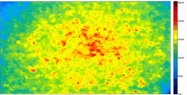
http://www.info2.uqam.ca/~makarenkov v/HTS/bome.pbp/downloa ds/Harvard 164.zip. .... .... . .... .. . . .. . ... .. . ... .... .. . . ... ... 29 1.2 Non-smoothed foreground (non-uniformity bias) for images of a

single (96-well x 4-field) HCS plate of microtubule polymerization status generated in the HCS laboratory of McGill university is shown. The data are available at http://nadon-mugqic.mcgill.ca . . . ... 30 1.3 Batch positional effect appearing in the McMaster Test assay

screened during the McMaster Data Mining and Docking Competition (Elowe et al. 2005). The first 24 plates of the assay are shown (12 original and 12 replicated plates; the plate number is indicated on each plate; the replicated plates are indicated by the letter R). Each original plate is followed by its replicate. Hits are shown in blue. Green boxes emphasize well (8, 9) on each plate (i.e., well H10, according to the McMaster annotation) where the batch effect occurs. The data are available at

http://www.info2.uqam.ca/~makarenkov v/HTS/home.pbp/downloa ds/McMaster l250.zip... 34 1.4 Proportion of rows and colurnns affected by systematic bias in 41

experimental HTS assays (735 plates in total; control wells were ignored) aiming at the inhibition of the Escherichia coli.

Experimental data were extracted from the Harvard University HTS databank (i.e., ChemBank (Seiler et al. 2008)). Here we show: (a) Overall row and colurnn error rate for raw data; (b) hit distribution surface error rates for raw data; ( c) overall row and colurnn error rate for background-subtracted data; ( d) hit distribution error rate for background subtracted data. The following hit selection thresholds were used to identify hits and establish hit distribution surfaces of the assays: j.1-2.5Π(0), j.1-3Π(t.) and j.1-3.5Π(o), where f1

and Πare, respectively, the mean and standard deviation of the

plate's measurements... 42

1.5 Recommended data pre-processing and correction protocol to be performed prior to the hit identification step in high-throughput and high-content screening... 49

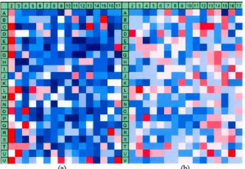
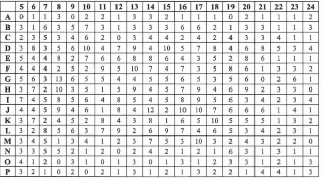
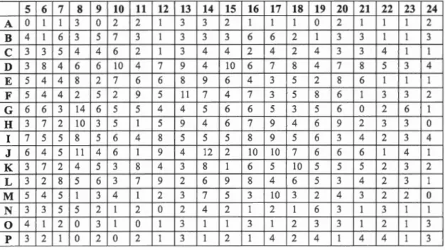
2.1 Edge effects in the RNAi HIV inhibition assay, screened at Pasteur Institute ofKorea (Carralot et al. 2012), shown within: (a) the assay hit distribution surface (i.e., overall hit counts per well location are depicted) and (b) Plate 7 raw activity levels. The hit selection threshold of j.1.-l.219Π(or 1% of hits) was used, where f1 and Πwere

the mean and the standard deviation of the plate measurements,

respectively. The samples whose measurements were lower than the threshold value were selected as bits. In (a), higher hit counts are in red and lower hit counts are in blue. In (b ), higher raw measurements are in blue and lower raw measurements are in red.

The non-target wells located in colurnns 1 to 4 were ignored in our analysis.... . . 57

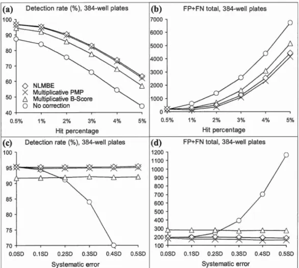
2.2 True positive rate, and combined false positive and false negative rate for 96-well plate assays obtained under the condition that a maximum of 4 rows and 4 colurnns of each plate were affected by spatial bias. Panels (a and b) present the results for datasets with the fixed standard deviation of spatial bias, equal to 0.3SD. Panels ( c and d) present the results for datasets with the fixed hit percentage rate of 1 %. . . 67

rate for 384-well plate assays. Figure 2.2 panel description applies here... .. . . ... 69 2.4 True positive rate, and combined false positive and false negative

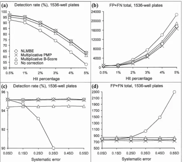
rate for 1536-well plate assays. Figure 2.2 panel description applies here... .. . . ... 70 2.5 True positive rate for 96, 384 and 1536-well plate assays and high

bit percentages (1% to 20%) obtained under the condition that a maximum of 4 rows and 4 columns of each plate were affected by spatial bias. Panels (a, c and e) present the results for datasets with the fixed standard deviation of spatial bias, equal to 0.3SD. Panels (b, d and f) present the results for datasets with the fixed bit percentage rate of 20%... 72 2.6 Hit distribution surfaces and Plate 7 heatmaps for the following

types of RN Ai HIV data: (a,g) raw data, (b,h) data corrected by the diffusion model, ( c,i) data corrected by additive B-score, ( d,j) data corrected only assay-wise, (e,k) data corrected only plate-wise using mPMP, and (f,l) data corrected both plate and assay-wise. The results for the bit selection threshold of j.1-1.219CT are depicted. Figure 2.1 description applies here... .. 78 2.7 Plate-specifie bias detected across the four HTS screenmg

categories available m ChemBank. 100 HTS assays (25 per screening category) were analyzed (see Supplementary Table ST12 for the ChemBank IDs of the assays). The control wells were removed from all screens prior to bias detection. The proportion of assays per screenmg category, affected by additive bias, by multiplicative bias, and by an undetermined type of bias is reported. No assays containing no biased plates at all were found in this ex periment... 81 2.8 Plate-specifie bias detected across 7 816 plates, including 3 001 344

gene expressiOn profiles, from the Normalized LlOOO mRNA profiling assay. The control wells were removed from all screens prior to bias detection. The proportion of plates affected by additive bias, by multiplicative bias, by an undetermined type of bias, as well as of those having no spatial bias at all, is reported. When the Mann-Whitney U test detected no any biased row or column in a g1ven plate, the plate was reported as containing no spatial bias... 83

SF1 Supplementary figure SF1 presents simulation results for 384-well plates with different control layouts (see the main text for more detail). Spatial bias was set to 0.3SD. The following plate layouts: (a) (16x24)-well plate with no contrais, (b) scattered controllayout (with 22 control wells - as shawn in Figure 2.1 b in (Mpindi et al. 20 15) and ( c) layout with 32 control wells, located in first and last columns of the plate (see Figure 2.1a in (Mpindi et al. 2015)), were

compared... . . 97 SF2 Plate 1 data corrected first assay-wise, and then plate-wise (using

aPMP)... .... ... . . . .. . . ... .. . . .... ... .... .... .. . ... . . . ... .. .. . . . .. 98 SF3 Plate 2 data corrected first assay-wise, and then plate-wise (using

aPMP)... 99 SF4 Plate 3 data corrected first assay-wise, and then plate-wise (using

aPMP)... ... 100 SF5 Plate 4 data corrected first assay-wise, and then plate-wise (using

aPMP)... .. . . ... 101 SF6 Plate 5 data corrected first assay-wise, and then plate-wise (using

aPMP)... ... ... 102 SF7 Plate 1 data corrected first plate-wise (using aPMP), and then

assay-wise... 103 SF8 Plate 2 data corrected first plate-wise (using aPMP), and then

assay-wise... 104 SF9 Plate 3 data corrected first plate-wise (using aPMP), and then

assay-WISe... 105 SF1 0 Plate 4 data corrected first plate-wise (using aPMP), and then

assay-wise... 106 SF11 Plate 5 data corrected first plate-wise (using aPMP), and then

assay-wise... 107 3.1 Proportion of plates with the indicated number of rows (A) affected

by spatial bias and number of co1umns (B) affected by spatial bias. The non-parametric Mann-Whitney U test was used to detect the presence of spatial bias within each plate... 121

3.2 Spatial bias model frequency based on evidence obtained from the Anderson-Darling test for high-throughput screening data (A)-(D),

high-content screening data (E)-(G) and small-molecule microarrays data (H). Control wells were excluded from all computations.

Darker portions of bars account for plates without intersections of rows and columns affected by spatial bias; in this case any additive mo del (Models 1-3) can be applied wh en spatial bias was classified as additive and any multiplicative model (Models 4-6) can be applied when spatial bias was classified as multiplicative. Lighter portions of bars corresponding to Models 1 to 6 account for plates with intersections of rows and columns affected by spatial bias (in this case, the model yielding the largest p-value should be applied)... 124 3.3 Spatial bias model frequency based on evidence obtained from the

Cramer-von-Mises test for high-throughput screening data (A)-(D), high-content screening data (E)-(G) and small-molecule microarrays data (H). Control wells were excluded from all computations. Darker portions of bars account for plates without intersections of rows and columns affected by spatial bias; in this case any additive model (Models 1-3) can be applied when spatial bias was classified as additive and any multiplicative model (Models 4-6) can be applied when spatial bias was classified as multiplicative. Lighter portions of bars corresponding to Models 1 to 6 account for plates with intersections of rows and columns affected by spatial bias (in this case, the model yielding the largest p-value should be applied)... 126

- --- -- - -- - - -- - - -

-LIST OF TABLES

T~k p~

0.1 Systematic biases specifie to HCS

technologies... 12 1.1 Data normalization methods recommended for the analysis of HTS

and HCS data, and classified according to the context in which they should be applied. The available software implementations are also indicated... ... . . .. 47 2.1 Number of hits found in the RN Ai HIV assay using: raw data (No

Correction), data corrected by diffusion model, data corrected by additive B-score, data corrected only assay-wise, data corrected only wise by mPMP, data corrected assay-wise and th en

plate-wise by mPMP, and data corrected plate-wise by mPMP and then assay-wise. The selected thresholds, ,u-1.3480", ,u-1.2930", ,u-1.2550"

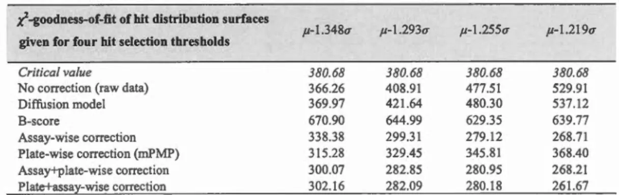
and ,u-1.2190", correspond to 1%, 2%, 3% and 4.13% of hits, respectively... ... 75 2.2 / goodness of fit statistic (given for a= 0.01) for the hit

distribution surfaces of the RNAi HIV assay computed after the application of the following data correction methods: No Correction, diffusion model, additive B-score, assay-wise correction only, plate-wise correction only by mPMP, assay-wise correction followed by plate-wise correction by mPMP, and plate-wise correction by mPMP followed by assay-wise correction. The selected thresholds, ,u-1.3480", ,u-1.2930", ,u-1.25 50" and ,u-1.2190",

correspond to 1%, 2%, 3% and 4.13% of hits,

respectively... 77 STl Hit distribution for the raw RNAi HIV dataset computed for the

j.l.-1.219SD ( 4.13%) threshold. This hit distribution surface is presented in Figure 2.6a of the main manuscript. Columns 1 to 4

were discarded because they did not contain target

compounds.. . . 86

mode! and computed for the ,u-1.219SD (4.13%) threshold. This hit distribution surface is presented in Figure 2.6b of the main manuscript. Columns 1 to 4 were discarded because they did not contain target compounds... .. . . ... . . .. . . .. 87 ST3 Hit distribution for the RNAi HIV dataset corrected by B-score and

computed for the ,u-1.219SD ( 4.13%) threshold. This hit distribution

surface is presented in Figure 2.6c of the main manuscript. Columns

1 to 4 were discarded because they did not contain target

compounds... . . 88

ST4 Hit distribution for the RNAi HIV dataset corrected assay-wise and

computed for the ,u-1.219SD (4.13%) threshold. This hit distribution

surface is presented in Figure 2.6d of the main manuscript. Columns

1 to 4 were discarded because they did not contain target compounds... ... . . ... . . ... . . 89

STS Hit distribution for the RNAi HIV dataset corrected plate-wise by

multiplicative PMP and computed for the ,u-1.219SD (4.13%)

threshold. This hit distribution surface is presented in Figure 2.6e of

the main manuscript. Columns 1 to 4 were discarded because they did not conta in target compounds. . . 90

ST6 Hit distribution of the RNAi HIV dataset corrected plate-wise by multiplicative PMP and then assay-wise and computed for the

,u-1.219SD (4.13%) threshold. This bit distribution surface is presented in Figure 2.6f of the main manuscript. Columns 1 to 4 were discarded sin ce they did not con tain target compounds... . . 91

ST7 Plate 1 raw measurements of the synthetic dataset presented in Section 2.2 of the main manuscript... 92 ST8 Plate 2 raw measurements of the synthetic dataset presented in

Section 2.2 of the main manuscript... 92 ST9 Plate 3 raw measurements of the synthetic dataset presented in

Section 2.2 of the main manuscript... 93 ST10 Plate 4 raw measurements of the synthetic dataset presented in

Section 2.2 ofthe main manuscript... 93 STll Plate 5 raw measurements of the synthetic dataset presented in

Section 2.2 of the main manuscript ... oo . . . 0 0 . . . 93 ST12 Set of 100 ChemBank assays analyzed in our bias detection

simulation described in Section 2.3 of the main manuscript (see also Figure 2.7 in the main text); 25 assays per HTS screening category (Cell-based, Homogeneous, Microorganism and Gene expression) were considered. . . 94

3.1 Contingency table of the number of plates affected by additive, multiplicative and undefined type of spatial bias, for the HTS, HCS and SMM technologies... 122

3.2 Set of 175 ChemBank assays examined in our plate-specifie bias

detection simulation (see Figs. 3.1-3.3). Note that only 8 non-empty HCS Area, 18 non-empty HCS Intensity and 24 non-empty HCS Cell count assays were available in ChemBank (as of April 14th, 2017). For all other screening categories, 25 assays per data category were examined ... 0 0 0 0 . .. . . 0 0 . . . .. .. . . 0 00 130

HTS HCS MAD eDNA RN Ai NLMBE SPAWN PMP mPMP CVM AD dsRNA siRNAs shRNAs esiRNAs

LIST OF ABBREVIA TI ONS AND ACRONYMS

High-Throughput Screening High-Content Screening Median Absolute Deviation Complementary DNA RNA interference

Non-Linear Multiplicative Bias Elimination Spatial Polish Well Normalization

Partial Mean Polish Multiplicative PMP Cramer-von-Mises test Anderson-Darling test double-stranded RNA small interfering RNA short hairpin RNA

RÉSUMÉ

Le criblage à haut débit (CHD) et le criblage à haut contenu (CHC) sont des techniques expérimentales efficaces permettant aux chercheurs d'identifier un petit nombre de candidats potentiels parmi des millions de composés chimiques (ou par exemple, de petites molécules, d'ADN complémentaire, de petits ARN interférents) pouvant devenir de nouveaux médicaments. Durant les dernières décennies, les nombreux centres CHD/CHC ont été créés dans les campus universitaires (Peter et Roy 2011). Au cours des dernières années, les résultats des CHD/CHC ont trouvé des grandes applications dans la recherche biologique, par exemple pour l'étude des maladies orphelines comme le paludisme et la fibrose kystique (Brewer 2009; Okiyoneda et Lukacs 2012; Preuss et al. 2012).

Néanmoins, les données CHD/CHC peuvent contenir des erreurs systématiques (ou des biais spatiaux). Ces erreurs affectent généralement de manière significative toutes les mesures expérimentales, en augmentant ainsi le nombre de faux positifs et de faux négatifs retournés pas des méthodes de recherche de composés actifs. L'application des méthodes statistiques appropriées permet d'éliminer ou de réduire l'effet d'erreurs systématiques dans les données CHD/CHC. Plusieurs chercheurs (Brideau et al. 2003, Makarenkov et al. 2007, Dragiev et al. 2011 et 2012) ont montré que les méthodes d'élimination des erreurs systématiques peuvent être appliquées avec succès

aux données CHD/CHC expérimentales. Dans cette thèse, nous proposons de

nouvelles méthodes et protocoles statistiques servant à réduire l'impact d'erreurs systématiques dans les analyses CHD/CHC. La thèse est divisée en trois parties principales correspondant à nos trois articles.

Le premier article examine les technologies de criblage existantes et leurs biais associes. Ici nous décrivons les différents types d'erreurs systématiques caractéristiques aux données CHD/CHC. Nous parlons de l'avantage des mesures répliquées et randomisées pour obtenir une meilleure précision des résultats dans les campagnes CHD/CHC. Les principales méthodes statistiques qui sont utilisées pour éliminer les erreurs systématiques, essentiellement de type additif, sont également

présentées. Dans ce premier article, nous évaluons la grandeur de l'erreur

systématique présente dans les données CHD expérimentales publics. Nous proposons également un protocole de prétraitement des données général, adopté à l'analyse des données de criblage.

Le deuxième article présente trois nouvelles méthodes statistiques pour éliminer les

erreurs systématiques multiplicatives. Pour détecter l'erreur systématique, nous utilisons le test non-paramétrique de Mann-Whitney U. Les biais spatiaux présents dans les essais sont corrigés via la résolution d'un système d'équations nonlinéaires

ou par les procédures itératives d'élimination de biais. Nous montrons que les nouvelles méthodes de correction de données suppriment bien des erreurs systématiques multiplicatives présentes dans les lignes et les colonnes de chaque plaque de l'essai considéré.

Le troisième article propose de nouvelles méthodes statistiques pour éliminer les

erreurs systématiques du type additif et multiplicatif, en considérant les différentes interactions possibles entre ces erreurs. Nous utilisons les tests de Cramer-von-Mises

et d'Anderson-Darling pour estimer la qualité de l'ajustement des valeurs originales

par des valeurs corrigées et pour déterminer ainsi le meilleur modèle pour les données d'intérêt.

MOTS-CLÉS : biais spatial, criblage à haut débit, criblage à haut contenu, erreur systématique, erreur additive, erreur multiplicative

SUMMARY

High-Throughput Screening (HTS) and High-Content Screening (HCS) are effective experimental techniques that allow researchers to identify a small number of potential drug candidates among millions of chemical compounds, cDNAs or RNAis. Over the last few decades, many HTS and HCS centers have been created in academie campuses (Peter and Roy 2011). Recently, HTS assays have also found large applications in biological research, e.g., in studying orphan diseases like malaria and cystic fibrosis (Brewer 2009; Okiyoneda and Lukacs 2012; Preuss et al. 2012). However, as bas been noted in many studies (Brideau et al. 2003, Makarenkov et al. 2007, Dragiev et al. 2011 and 2012), HTS and HCS data are usually severely affected by systematic errors (i.e., spatial biases). These errors lead to an important increase in the number of false positive and false negative bits ( e.g., active compounds that have the potential to be developed into new medications). One possible solution to this problem is to apply statistical methods designed to minimize the impact of systematic errors on experimental HTS/HCS data. To this end, this thesis proposes new statistical methods, data pre-processing protocols, and software for reducing systematic errors from experimental high-throughput screening assays. The thesis is organized by publications.

The first paper reviews existing screening technologies and their related biases. It

describes the different types of systematic errors present in HTS and HCS data. The existing statistical methods and models proposed to eliminate systematic errors are also reviewed. In the first article, we also assess the magnitude of systematic error in experimental HTS data and propose a general data pre-processing protocol which can be recommended for the analysis of the current or next generation screening data. The second paper presents three new statistical methods for spatial bias correction meant to minimize the impact of multiplicative spatial biases. In our study, the presence of bias in rows and colurnns of a given plate is identified using the non-parametric Mann-Whitney U test. Our data correction methods modify the data only in the bias-affected rows and colurnns. The usefulness of the new methods is demonstrated by a simulation study as well as by the analysis of publicly available ChemBank data.

In the third paper, we consider six bias correction models: two existing models and four new models. These models account for different possible interactions between additive and multiplicative spatial biases. We use the Cramer-von-Mises and Anderson-Darling tests to estimate the goodness-of-fit of the raw data by the corrected data and to select the most appropriate (additive, multiplicative or mixed) spatial bias model for the data at hand.

K.EYWORDS: high-throughput screening, high-content screening, systematic error,

INTRODUCTION

0.1. High-Throughput Screening and High-Content Screening

High-Throughput Screening (HTS) and High-Content Screening (HCS) are popular biotechnological methods allowing researchers to test a large number of chemical compounds in order find a small proportion (around 1% or less) of potential drug candidates (i.e., chemical compounds with very high activity levels, also called bits). Nowadays, HTS and HCS assays are regularly used by the modem pharrnaceutical industry at the first step of the drug discovery process (Dove 2003; Kaiser 2008; Silber 201 0; Lachmann et al. 20 16). It bas been also demonstrated that the se technologies can be used successfully for studying various diseases, including the orphan diseases like malaria and cystic fibrosis (Brewer 2009; Okiyoneda and Lukacs 2012; Preuss et al. 2012). As indicated in Malo et al. (2006) and Sirois et al. (2005), the drug development process usually contains the four following main steps (Figure 0.1):

1. Primary Screen: preparation of screening assay and primary bit detection; 2. Counter screen and Secondary screen: bit identification for biological

relevance and bit confirmation;

3. Structural-activity relationship (SAR) and medical chemistry: identification of leads;

4. Clinical trials: clinical compound selection, entry into human studies and regu1atory approval for a new drug.

A blological assay

(specifie target

& reagents) Prtmary screen

'Hils'

Secondary screen & œunter screen

'Confirmed hils'

Structure-activity relationshJp (SAR)

& medicinal chemistry

.-~-~ 'Lea{js' 'Drug' A large library of chemicaJ compounds

Figure 0.1 The drug development process according to Malo et al. (2006).

During a typical HTS/HCS campaign, lasting over a few days, millions of chemical compounds and thousands of microtiter plates are usually analyzed (Agresti et al. 2010).

3

In an HTS/HCS pnmary assay, the selected library of chemical compounds is

screened against a specifie biological target to measure the intensity of the related inhibition or activation signal.

Figure 0.2 presents typical HTS plates. In general, a standard HTS plate contains either 96, or 384, or 1536 wells.

Figure 0.2 Typical HTS plates (96 wells, 384 wells and 1536 wells, respectively); source: https://shop.gbo.com/en/row/products/0110/0110_0040.

The wells are arranged in a rectangular matrix pattern. The robots introduce an appropriate biological target culture into every well of a given plate, such as a protein, a small molecule, a cell, or a siRNA. After the incubation period, the measurements are taken to get the evaluations of biological activity in all wells of the plate using specialized automated analysis machines. The measurement of a well is usually considered as a single numeric value. Thus, the measurements of a plate obtained during the screening process can be represented by a matrix of numerical values. At the end of the screening process, statistical methods should be used to find the hits (i.e., the compounds with the highest activity levels).

E.coli bacterium Ce lis Aeooooooooooe eeooooooooooe ceooooooooooe oeooooooooooe Eeooooooooooe Feooooooooooe G• ooooooooooe Heooooooooooe B. ,,. c: 100 .,.·,. .... ~_.,. .... ,. ... .,..._ .. • •••• ~ 10 ~ .! " z-.ru:tor • 0.19 ~ .-o n-48 ~ 10 ~ 0 .

.

.

,.

Plates containing cell culture of interest A000000000000 BOOOOOOOOOOOO coooooooooooo D 000000000000 EOOOOOOOOOOOO F000000000000 G000000000000 H000000000000 Automated processing and scanning

Figure 0.3 A typical HTS/HCS procedure. Blue colored wells contain negative controls, red colored wells contain positive controls and yellow colored wells contain

the library compounds.

Figure 0.3 presents an example of a typical HTS/HCS process (Menke 2002; Janzen

and Bemasconi 2009; Macarr6n and Hertzberg 2011). This process uses the robotic

liquid handling, automatic processing and scanning of plates, as well as sorne

statistical tools to detect chemical compounds (i.e., bits) providing the best inhibition of the E. coli bacterium. The presented assay uses 96-well plates.

5

Figure 0.4 HTS robotic equipment usmg hundreds of pipettes; source:

http:/ /whyfiles.org/20 14/stem-cell-advance.

Recent improvements in drug discovery and in high-throughput screening permitted obtaining high resolutions even at the cellular level (Noah 201 0). The corresponding screening technology was named High-Content Screening (HCS). The detailed information about cell structure can be now obtained by extracting multicolor fluorescence signais. The main sub-categories of HTS and HCS technologies are the following: small molecules, complementary DNAs (cDNAs), and RNA interference (RNAis). These sub-categories vary with respect to the target of interest.

In the pharmaceutical industry the term small molecule is related to a specifie biological target such as a specifie nucleic acid or protein (Cram101, 2012). Small -molecules are used in drug discovery for target validation, assay development, secondary screening, pharmacological property assessment and lead optimization (Lazo et al. 2007). eDNA libraries are manufactured from messenger RNAs (mRNA molecules) (Brown and Song 2000). The transformation ofunstable mRNA template,

via reverse transcription, produces stable eDNA. Nowadays, the eDNA libraries are a very effective tool used in drug discovery. The biological process, in which a short RNA molecule suppresses gene expression by targeting specifie mRNA molecules for degradation is defined as RNA interference (RNAi). The researchers call this process silencing. This technique is frequent in drug discovery. Scientists use the RN Ais to silence genes. Nowadays, four types of RN Ai rea gents are applied in RN Ai screening technologies: dsRNAs (double-stranded RNA), siRNAs (small interfering

RNA), shRNAs (short hairpin RNA), and endoribonuclease-prepared siRNAs

(esiRNAs) (Mohr et al. 2010).

A more detailed description of small molecule, eDNA and RN Ai screens is available in Chapter I. The main biases characteristic for these screens are presented in details in Section 0.3.

0.2 Systematic error in HTS/HCS screens

Unfortunately, raw compound activity measures can be disturbed by two additional factors: random errors and systema.tic errors (or spatial biases) (Makarenkov et al. 2007). Random error lowers screening precision and may affect false positive and false negatives rates (Box et al. 2005). Its negative impact can be minimized by using duplicate measurements (Malo et al. 201 0) or by blocking (Murie et al. 20 15). Ramadan et al. (2007) showed that random errors can be the cause of nonspecific phenotypes in specifie wells and lead to higher rates of false positives and false negatives. In contrast, Dragiev et al. (2011) suggested that random error, on the opposite of systematic error, usually bas a minimum impact on the hit selection process.

7

Definition Systematic error, or systematic bias, can be defzned as a variability of measurements taken at the same plate or assay locations, consisting of their systematic under or over-estimation (Kevorkov and Makarenkov 2005).

Systematic error, or systematic bias, has been observed in many HTS/HCS assays (Brideau et al. 2003, Makarenkov et al. 2007, Lachmann et al. 2016). The origin of systematic error can be biological, human or mechanical. For instance, it can be due to different robotic and environmental factors, such as robotic failure, reader effect, pipette malfunctioning or other liquid handling anomalies, variation in the incubation time or temperature difference, and lighting or air flow abnormalities, present over the course ofthe entire screen (Heyse, 2002; Makarenkov et al., 2007).

Different types of systematic error, including edge and batch effects (Soneson et al. 2014 ), are described in detail in Chapter I of this thesis.

0.3 Small molecule, eDNA and RNAi screens and the related systematic errors

Small molecule screens: Small molecules can be either natural or artificial. These molecules are associated with a particular biopolymer. Kim et al. (2007) showed that a lot of small molecules are cytotoxic in hepatocyte replicon cell lines. These molecules are very susceptible to cytotoxic or cytostatic agents. Cytotoxic effects may be confused with antiviral activity when cytotoxic effects have lower luciferase signal reducing cells' vital activity. Chan et al. (2009) indicated that a substantial fraction of small molecules show aggregating behaviour. It usually happens because of nonspecific attachment to target proteins, resulting in false positive bits in experimental screening assays. Thus, the capability to effectively detect the substances with aggregating characteristics may rationalize the screening procedure by excluding uns table molecules from further examina ti on. Harmon et al. (20 1 0) indicated that many pathogenic Gram-negative bacteria represent a type three

secretion system (TTSS). TTSS translocates effectors proteins into the cytosol of their eukaryotic cell targets. The authors mentioned that the molecules that interfere with assembly of TTSS are not efficiently detected in experimental HTS screens. They postulated that systematic error in small molecule screens often appears due to the fact that TTSS is preassembled prior to exposure to compounds and cells. Wootten et al. (20 13) mentioned that the individual G protein-coupled receptor (GPCRs) may be found in multiple receptor conformations and may be the cause of numerous functional reactions, bath G protein- and non G protein-mediated. This concept, referred to as biased agonism, is also known as functional selectivity, or stimulus systematic bias, or ligand-directed signaling, or ligand systematic bias (Kenakin 2011). We should mention that sorne interesting cases of ligand systematic bias for the glucagon-like peptide-1 were discussed in Willard et al. (20 12).

eDNA sereens: eDNA libraries are essential tools for discovery and validation of novel drug targets in functional genomics applications, but they are not exempt of different biases. In one of earlier studies, Kopczynski et al. (1998) suggested that the representation of clones is underestimated or overestimated by sequence analysis encoding membrane-targeted proteins in the rough microsomes libraries. It happens due to systematic error related to cytosolic and nuclear proteins. Caminci et al. (2000) indicated that the process of generating full-length eDNA libraries may have sorne specifie issues. The authors mentioned that the process of preparation a full-length eDNA is more effective for short mRNAs than for long transcripts. Moreover, cloning and propagation are trickier for long cDNAs than for short cDNAs, therefore creating further size bias. Carninci and Shibata (2000) observed that the plasmid libraries were related to a cDNA-size cloning bias. This bias manifests itself as an increased cloning effectiveness of short cDNAs. Furthermore, the increase of eDNA clones can be related to the plasmid length during library amplification before normalization and/or subtraction. It means that the long clones are usually underrepresented after bulk amplification of the library. To overcome the issues

9

related to the library amplification, Carninci and Shibata developed a specifie eDNA data correction method. Fossa et al. (2004) demonstrated the aptitude of biopanning to enrich TAAs (tumor-associated antigens) from tumor eDNA libraries under determined experimental conditions. However, this enrichment may be related to the loss of positive clones as weil as to systematic error. Systematic error arises here from non-immunological factors (for example: inefficient protein presentation or delayed growth of phage-infected bacteria). Wan et al. (2006) suggested that the oligonucleotide synthesis is not entirely effective. It means that the probability of the presence of synthesis bias augments with every base added. Wan et al. suggested using only high-quality oligonucleotides because synthesis bias may be either included into the amplified product or may generate sorne other off-target effects.

RNAi screens: Recently, RNA interference (RNAi) screemng has made great

progress, evolving from a biological phenomenon into an effective method of drug discovery (Sharma and Rao 2009). Birmingham et al. (2009) mentioned that the transfection process is the main source of variability in siRNA screens. Transfection process produces cell stress and influences cell viability. It may have variable and indirect phenotypic influence in cellular assays. The target gene product can be decreased or practically erased in the cell by RNAi reagents. Due to these mechanistic factors, RNAi reagents require 48-72 hours for maximal effect, whereas small molecules can immediately affect their protein targets within a few hours. Such longer time intervals between cell plating and assay endpoint lead to a greater impact of cell culture and environmental variation on phenotypes and cause sorne important assay variability in RNAi screens. Zhang et al. (2008) underlined that a good plate design in HTS RNAi is needed to identify systematic error as well as to determine which normalization and data correction techniques should be used to reduce the impact of systematic error on both quality control and hit selection processes. Auer and Doerge (20 1 0) discussed so-called fane effect in RN Ai screens. The authors indicated that lane effect includes any systematic error that appear from the item at

which the sample is introduced into the flow cell until the samples are removed from the sequencing machine (i.e., badly-organized sequencing cycles and errors in base calling). Several publications have appeared in recent years to highlight that the main issue in RNAi screening is off-target effect (Birmingham et al. 2006; Buehler et al. 2012; Chen et al. 2013; Das et al. 2013). This kind of error appears when a siRNA is processed by the RNA-Induced Silencing Complex (RISC) and down-regulates unintended targets. Echeverri et al. (2006) suggested that an initial origin of off-target effects is a comparatively buge tolerance for mismatches between the siRNA guide strand, the ultimate targeting molecule and the complementary target mRNA sequence, outside of the short 'core' targeting region. Sharma and Rao (2009) described three different types of off-target effect. Firstly, when a siRNA sequence is the same or nearly identical to a sequence present in an unrelated mRNA, the final degradation of the unrelated mRNA can establish a confounding phenotype. Thus, the final result is a false-positive hit. We can avoid this problem only if the related siRNA sequences are selected very carefully. Secondly, a siRNA may operate as microRNA and produce depletion of non-target proteins through mRNA degradation or translational block, where the 'seed region' of a siRNA pairs with a weakly complementary sequence in the 3' untranslated region of an unrelated mRNA. This problem is intrinsic to RNAi screens and is very difficult to solve. The last type of off-target effect is characteristic for mammalian cells. It is well known that even short siRNA can switch on the antiviral type I interferon response in a sequence-independent way, particularly when saturating doses of siRNA or shRNA are supplied.

0.4 Systematic errors specifie to HCS

HCS-specific systematic biases can be divided into two types according to their spatial distribution (see Table 0.1):

11

1. Intra-well (per weil) bias appears when cells are not distributed uniform1y. It is arising while gathering data from a given well location. It usually happens when cells are clumped, which also changes cell adherence and morphology characteristics. Such an effect is called cel! count distribution systematic bias. It affects post-processing steps and can skew results significantly if not enough images per well are taken. Another type of intra-well bias can appear because of cell cycle distribution heterogeneity when cells are in different stages of cell cycle, and thus treatments are affecting them differently. This usually bas an effect when analyzing treatment response and cell structure (Snijder and Pelkmans 2011 ).

2. Intra-image (per-image) bias consisting of microscope-related errors is ar1smg while capturing images. One of the issues here is a non-uniformity of background light intensity distribution, which is slowly varying as well as systematic change of the spatial distribution of light in images. Such an effect can add or subtract intensities at any pixel location, thus affecting data quantification and statistical analysis, which, in turn, can affect cell segmentation and florescence measurements (Lo et al. 2012).

Systematic bias can also occur if the focus is not maintained throughout all captured images. Out of focus images can impact on the cell segmentation (Bray et al. 2012). They can also lead to the issues in the identification of thresholds that consistently separate abjects of interest from background, thus reducing the accuracy of object segmentation and causing bias in the measured cell metrics that depend on both the pixel intensities and segmentation step (Lo et al. 2012). It is worth noting that image segmentation is vital for the viability HCS data. Identification of cells or sub-cellular structures and the related morphological "features" (such as fluorescent intensity,

object shape, size and texture) are fully dependent on image segmentation. We should mention that, unfortunately, sorne "HCS-unfriendly" cell lines, which are still very clinically pertinent, for example human tumor cell line SK-BR-3, grow only in

complex patterns. For such cell tines, one must be very careful when doing image

segmentation, because errors in segmentation can arise more frequently, resulting in

the inappropriate designation of partial or multiple cells as single cells.

Another comrnon problem in HCS is that of fluorophore saturation and debris, which can affect the intensity measurement. It can occur if the settings are not optimal for every image, resulting in a higher than maximum signal for at least one pixel. Such

an effect reduces the measured intensity value of the affected pixel, systematically

biasing the intensity results (Brown 2007). In a typical HCS screen, in which

hundreds or thousands of images are segmented, the review, classification and

correction of the acquired images is a complex task requiring multiple statistical and medical skills. Systematic errors in these screens should be removed using appropriate correction and normalization methods (Hill et al. 2007).

Table 0.1 Systematic biases specifie to HCS technologies

Per weil intra-well) Per image (intra-image)

Out-of

Non-uniformity Fluorophore

Cel/ coLm/ distribution Cel/ cycle distribution focus

systematic bias saturation

bias and debris

Clumping of Ce lis Morphology- Ce li Intensity

ce lis adherence related error structure Segmentation error measurement

error err or error

0.5 Data normalization methods

Normalization techniques used m HTS/HCS allow for transforming the

measurements of a given plate (orwell location) in order to make them comparable

over different plates (or well locations) of the same assay. We should mention that

13

errors. The following simple normalization methods are commonly used in HTS/HCS technologies:

Z-score: is a simple and well known method which allows one to transform the original data set into a normalized data set with the mean of 0 and the standard deviation of 1. The mean value of a given plate is first subtracted from all of its measurements. After that the values of all measurements are divided by the standard deviation of the plate. The equation that describes Z-score is as follows:

A x if

-11 _{h e " d ct· el th mean and the standard}

x if

=

deviation the plate's measurements.

Robust Z-score: is similar to Z-score, but uses the MAD statistic instead of the standard deviation of the plate. Also, in the Robust Z-score the median is applied in place of the mean to get a more robust statistical estimate. Robust Z-score

x-med

normalization is described by the following equation:

x

..

=

the median of all measurements of a given plate and MAD is its Median Absolute Deviation. The robust Z-score normalization is more robust to outliers compared to traditional Z-scores. For more details about the existing data normalization techniques the reader is referred to Chapter I.

0.6 Statistical tests to detect the presence of systematic error in screening data

Once the raw experimental data are normalized, statistical tests can be applied to them to detect the presence of systematic error. These tests allow for a judicious use of bias elimination methods and software which should be applied with caution. Makarenkov et al. (2007) indicated, for example, that spatial bias correction methods may introduce different biases into the data at band when applied to bias-free data. We will actively use bias detection techniques in Chapter II, in which we present new

bias correction methods assuming that the biased rows and colurnns of all plates are known. The main tests that have been used for bias detection in screening technologies are summarized below:

Welch's t-test (Welch 1947) is an adaptation of Student's t-test. This test does not assume that the two data samples are drawn from populations with equal variances and that these populations have the same size. The measurements of a particular plate (or of a hit distribution surface) are divided into two samples: the first sample includes the values of the tested row or column and the second sample includes the rest of the plate's measurements. The null hypothesis, H0, here is that the considered

row or column does not contain systematic error. The equation that defines Welch's t-test is as follows: t

=

2 2

!.L+~

N₁ N₂

into two samples: S, - the first sample that includes the measurements of the tested row or column and S₂ - the second sample that includes the rest of the plate's

measurements. Here, f.1.1 is the mean of sample S, and f.1.z is the mean of sample S2, sample S, contains N, elements and sample S2 contains N2 elements, and s~ and

si

The Mann- Whitney U test is equivalent to the Wilcoxon rank sum test (Wilcoxon

1945; Gibbons and Chakraborti 2011). lt is a nonparametric test. As in many other nonparametric procedures, the ranks of the scores are calculated. W e combine two populations and we assign the rank to each of the scores. The first lowest measurement obtains rank 1; the second lowest measurement gets rank 2, and so on. This procedure verifies the null hypothesis, Ho, which postulates that the two compared population distributions are identical.

The Kolmogorov-Smirnov goodness-of-fit test (D'Agostino and Stephens 1986)

15

1965; a1so see Dragiev et al. 2011). To apply the DFT procedure to raw data we need first to unroll the plate's measurements matrix into a linear sequence of measurements. There are two natural ways to do so:

• to construct this sequence beginning with the first row of the plate, followed

by the second one, and so on, and

• to construct this sequence beginning with the first colurnn of the plate,

followed by the second one, and so on.

DFT detects frequencies of signais that repeat each two, three, four, and so on,

positions in the sequence and computes the amplitudes of each eventual frequency component. We apply the Kolmogorov-Smimov goodness-of-fit test to calculate the

density spectrum

y{

statistic D can be determined usmg the following equation:

D=

(F(y{)

-k-

1

,!5_-F(y{

)),

F(y{)

I<;,k<;,Nx(NR+Nc) N N

measurements in the density spectrum that are lower than or equal to

y{.

D are large, this suggest the rejection of the null hypothesis which postula tes that the tested measurements have been drawn from random normally distributed data.

0.7 Systematic error correction methods used in screening technologies

The main purpose of systematic error correction methods is to eliminate the

plate-specifie and assays-specific spatial biases within the considered plate or assay.

Plate-specifie biases affect the data located in a particular row or colurnn of a given plate.

Assay-specifie biases affect the data of the same weil location over ali plates of a given assay. Here, we present the most important methods, which have been used for bias correction in the HTS/HCS technologies. More methods are presented in Chapter I of this thesis.

R-score: The robust regression procedure is used to fit the regression model to the data in the R-score method. To assess the method's parameters, the rlm function from the MASS package of the R statistical language is applied. The equation that describes the R-score model (Wu et al. 2008) is as follows: xiJP

=

+

+

+

where xiJP is the compound measurement in row i and columnj of plate p, Jlp is the mean of plate p, R;p is the row bias affecting row i of plate p, C_1p is the column bias affecting column j of plate p, and rup is the residual in well (i,j) of plate p.

B-score: On the p111 plate, the residual riJp = xiJP-xiJP of the measurement located on

the intersection of row i and column j is calculated by applying a two-way median polish procedure (Tukey 1977; Brideau et al. 2003 ). The residu al is obtained as the difference between the raw value XiJp and the fitted value xiJP. The model is defined as

follows: xiJP

=

+

+

+

rup's. The B-score estimates are obtained from the following equation: r..

B-score = ~ where MAD P = med {1 riJP - med (riJP) 1}. p '

Partial Mean Polish (PMP): PMP (Dragiev et al. 2012), or additive PMP, is another extension of the well-known median po1ish procedure (Tukey 1977). PMP is an iterative method, in which the measurement correction is applied only to the rows and columns of a given plate that are affected by spatial bias (the bias location is assumed to be known in this method).

Weil correction: This is an assay-specifie correction method that normalizes the data along the well locations of a given assay (Makarenkov et al. 2007). At first, Z-score normalization is carried out within each plate of the assay. Th en, a linear !east-square approximation is carried out for the measurements of each weil location of the assay.

17

Finally, Z-score normalization is applied once agam, but this time for the measurements of all weil locations of the assay.

Diffusion Mode!: This method was designed to minimize the edge effect in the HTS RNAi screens (Carralot et al. 2012). The method relies on a diffusion model using the

Laplace operator:

ob(i,j,t) =

cx

f..

x

b(i,J

,t), where

b(i

,

j

,t)

spatio-ot

temporal diffusion field in well (i, j) at time t (i.e., evaluated spatial bias), c is the diffusion coefficient, and f.. is the Laplace operator.

Spatial and Weil Normalization (SPA WN): The SPA WN method first applies a

trimmed mean polish procedure on individual plates to minimize row and colurnn (i.e., plate-specifie) spatial biases (Murie et al. 20 13). It was shown that the trimmed mean approach has good a robustness (Malo et al. 2010; Murie et al. 2015). The R-score model is used to fit the data. Second, a well normalization step is carried out to determine spatial bias template, using the median of the scores at well location (i, j)

computed over all plates of the assay. The spatial bias template scores are subtracted from the scores obtained by the median polish procedure. Th us, SPA WN allows one to minimize both plate-specifie and assay-specifie spatial biases.

0.8 Hit identification

The goal of any HTS/HCS campaign is to identify the compounds with the highest activity levels (i.e., hits). Statistical and bioinformatics tools can allow practitioners to ameliorate the precision and exactitude of the detected hits using an appropriate experimental design and analytical methods. This data analysis step is critical in high-throughput screening.

Sorne practitioners select as screenmg positives a fixed number, or a fixed percentage, of top scoring compounds (for example 1%, Nelson 2004). Compounds

whose activity exceeds a fixed percent-of-control threshold may also be considered as bits (Malo et al. 2006). A key limitation of this strategy is that it is rather arbitrary and suffers from the absence of any probability model.

The second strategy for bits detection is to find the compounds whose activity exceeds a threshold that is a function of the mean and the standard deviation of the data at band. As reported by Makarenkov and Zentilli (Makarenkov et al. 2007), the bit selection thresholds are usually established using the fl-CCJ formula for inhibition

assays (here the bits are the values that are lower than this threshold) and fl+CCJ

formula for activation assays (here the bits are the values that are higher than this threshold), where the mean value fl and the standard deviation CJ are computed separately for each plate. The constant c is usually set to 3.0, 2.5 or 3.5.

A number of more robust statistical strategies for the bit identification have been described by Malo et al. (2006) and Birmingham et al. (2009). Among them we can mention the Random Variance Mode! (RVM, Wright and Simon 2003), the quartile-based bit identification procedure in RNAi screens, which establishes upper and lower bit selection thresholds based on number of interquartile ranges (Zhang et al. 2006), and an accurate Strictly Standardized Mean Difference (SSMD) method, calculating the ratio between the difference of the means and the standard deviation of the difference between positive and negative controls (Zhang 2007).

For more details about the existing bit identification techniques the reader is referred to Chapter I.

19

0.9 Data randomization and replicate measurements

Randomization is a very important part in a number of experimental technologies. In 1925, Fisher introduced the concept ofrandomization in which experimental units are assigned to groups or treatment in a manner that the probability of assignment to any particular group or treatment is equal and unbiased (Fisher 1925). The work of Fisher indicates that the placement of testing units has to depend on a random unbiased process. The main advantage of randomization in screening technologies is that randomized experimental units can distribute the error in a way that does not introduce discrepancy to the experiment (Box 2006; Hall 2007; Murie et al. 2015). Consequently, the compound placement, both within each plate and each well

location of an HTS assays, should be randomized in order to reduce the impact of systematic compound placement on the outcome of screening experiments.

The hit identification accuracy can be also improved using replicates. Replicates offer the twin advantage of obtaining a greater precision of activity measurements and that of estimating the measurements variability (Malo et al. 2006). Due to the cost issue, primary screens each compound is usually evaluated only once. But in secondary screens the use ofreplicates is strongly recommended (Murie et al. 2013). We should mention that Malo et al. (2006) recomrnended the application of replicates even in primary screens. Nowadays it is standard practice to get at least three replicates per measurement, assuming that these replicates provide the benefits which exceeds the cost of short-dated considerations (Lee et al. 2000; Nadon and Shoemaker 2002).

Obviously, replicated samples in HTS/HCS screens should be evaluated under the identical experimental conditions.

A detailed discussion of the advantages of the data randomization and replication procedures is provided in Chapter I.