https://doi.org/10.5194/cp-14-473-2018
© Author(s) 2018. This work is distributed under the Creative Commons Attribution 3.0 License.
Arctic hydroclimate variability during the last 2000 years:
current understanding and research challenges
Hans W. Linderholm1, Marie Nicolle2, Pierre Francus3,19, Konrad Gajewski4, Samuli Helama5, Atte Korhola6, Olga Solomina7, Zicheng Yu8, Peng Zhang1, William J. D’Andrea9, Maxime Debret2, Dmitry V. Divine10,18, Björn E. Gunnarson11, Neil J. Loader12, Nicolas Massei2, Kristina Seftigen1,13, Elizabeth K. Thomas14,
Johannes Werner15, Sofia Andersson11, Annika Berntsson11, Tomi P. Luoto16, Liisa Nevalainen16, Saija Saarni17, and Minna Väliranta6
1Regional Climate Group, Department of Earth Sciences, University of Gothenburg, 40530 Gothenburg, Sweden 2Normandie Univ, UNIROUEN, UNICAEN, CNRS, M2C, 76000 Rouen, France
3Institut National de la Recherche Scientifique, Centre Eau Terre Environnement, G1K 9A9, Québec, QC, Canada 4Département de géographie, Université d’Ottawa, Ottawa, Ontario K1N 6N5, Canada
5Natural Resources Institute Finland, Rovaniemi, Finland
6Environmental Change Research Unit (ECRU), Department of Environmental Sciences, University of Helsinki,
00014 Helsinki, Finland
7Institute of Geography, Russian Academy of Sciences, 119017 Moscow, Russia
8Department of Earth and Environmental Sciences, Lehigh University, Bethlehem PA 18015-3001, USA 9Lamont-Doherty Earth Observatory, Columbia University, Palisades NY 10964, USA
10Norwegian Polar Institute, Fram Centre, 9296 Tromsø, Norway
11Department of Physical Geography, Stockholm University, 10691 Stockholm, Sweden 12Department of Geography, Swansea University, Swansea SA2 8PP, Wales, UK
13Earth and Life Institute, Université catholique de Louvain, 1348 Louvain-la-Neuve, Belgium 14Department of Geology, University at Buffalo, Buffalo NY 14260, USA
15Department of Earth Science, University of Bergen, 5020 Bergen, Norway
16Department of Environmental Sciences, University of Helsinki, 15140 Lahti, Finland 17Department of Geography and Geology, University of Turku, 20014 Turun yliopisto, Finland
18Department of Mathematics and Statistics, University of Tromsø – The Arctic University of Norway, 9037, Norway 19GEOTOP Research Center, Montréal, QC, Canada
Correspondence:Hans W. Linderholm (hans.linderholm@gvc.gu.se) Received: 9 March 2017 – Discussion started: 17 March 2017
Revised: 9 January 2018 – Accepted: 20 February 2018 – Published: 10 April 2018
Abstract.Reanalysis data show an increasing trend in Arc-tic precipitation over the 20th century, but changes are not homogenous across seasons or space. The observed hydro-climate changes are expected to continue and possibly ac-celerate in the coming century, not only affecting pan-Arctic natural ecosystems and human activities, but also lower lati-tudes through the atmospheric and ocean circulations. How-ever, a lack of spatiotemporal observational data makes re-liable quantification of Arctic hydroclimate change difficult, especially in a long-term context. To understand Arctic
hy-droclimate and its variability prior to the instrumental record, climate proxy records are needed. The purpose of this re-view is to summarise the current understanding of Arctic hy-droclimate during the past 2000 years. First, the paper re-views the main natural archives and proxies used to infer past hydroclimate variations in this remote region and out-lines the difficulty of disentangling the moisture from the temperature signal in these records. Second, a comparison of two sets of hydroclimate records covering the Common Era from two data-rich regions, North America and
Fennoscan-dia, reveals inter- and intra-regional differences. Third, build-ing on earlier work, this paper shows the potential for pro-viding a high-resolution hydroclimate reconstruction for the Arctic and a comparison with last-millennium simulations from fully coupled climate models. In general, hydroclimate proxies and simulations indicate that the Medieval Climate Anomaly tends to have been wetter than the Little Ice Age (LIA), but there are large regional differences. However, the regional coverage of the proxy data is inadequate, with dis-tinct data gaps in most of Eurasia and parts of North America, making robust assessments for the whole Arctic impossible at present. To fully assess pan-Arctic hydroclimate variabil-ity for the last 2 millennia, additional proxy records are re-quired.
1 Introduction
Global climate is changing rapidly, largely due to increased anthropogenic greenhouse gas emissions (IPCC, 2013). However, distinct regional differences in the magnitude of observed warming in recent decades are apparent; for ex-ample, the Arctic has warmed at more than twice the rate of the global average (Cohen et al., 2014). This Arctic am-plification(Serreze et al., 2009) is due to complex feedback processes within the atmosphere–cryosphere–ocean system, including surface albedo and heat exchange with the ocean (Johannessen et al., 2003; Hind et al., 2016) and, most im-portantly, substantial losses of sea ice extent and late-spring snow cover (Overland, 2014).
Temperature increases have resulted in an intensified hy-drological cycle (Huntington, 2006). Increasing precipitation in the Arctic has been linked to higher local evaporation and reduced sea ice coverage (Bintanja and Selten, 2014; Kopec et al., 2016), but also enhanced northward transport of moisture (Zhang et al., 2013). According to most climate models (see Sect. 2), precipitation will continue to increase in the coming century, with the largest changes occurring over the Arctic Ocean (Bintanja and Selten, 2014). However, there are still large uncertainties regarding hydroclimate vari-ability and changes in the hydrological cycle in the Arctic due to incomplete or fragmentary data (Serreze et al., 2000; Screen and Simmonds, 2012). This makes it difficult to de-tect changes in and understand the mechanisms controlling hydroclimate variability on different timescales.
There are large spatial differences in the meteorologi-cal station distribution across the Arctic, and except for Fennoscandia and westernmost Russia, only a few obser-vational records reach more than 75 years back in time (Bekryaev et al., 2010), making it difficult to provide a spa-tiotemporal understanding of hydroclimate variability. Go-ing beyond the observational records, climate proxies are needed. Most reconstructions of past climate for the whole Arctic during the Common Era (CE) have focused on temper-ature (Overpeck et al., 1997; Kaufman et al., 2009; Shi et al.,
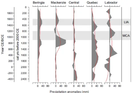
2012; Hanhijärvi et al., 2013; McKay and Kaufman, 2014). However, a number of proxies recorded in natural archives, such as ice cores, lake and peat sediments, and tree rings, can provide information on hydroclimate variations in the Arctic. They provide information with different temporal and sea-sonal resolution. In a recent study of hydroclimate variability across the Northern Hemisphere during the last 1200 years, Ljunqvist et al. (2016) found a tendency for generally wet-ter conditions during the 9th–11th centuries corresponding to the Medieval Climate Anomaly (MCA, ca. 900–1150 CE), whereas the 12th–19th centuries, including the Little Ice Age (LIA, ca. 1400–1850 CE), showed more widespread dry con-ditions. However, for the Arctic, only 18 records with het-erogeneous spatial distribution were included. Nevertheless, ongoing efforts to collect new data have resulted in a grow-ing network that will increase our understandgrow-ing of Arctic hydroclimate variability.
The aim of this review is to summarise the current under-standing of Arctic hydroclimate, focusing on the last 2 mil-lennia. The paper uses the PAGES 2k definition of the Arctic, i.e. the region north of 60◦N. Section 2 briefly presents the current state and a future outlook of Arctic hydroclimate and impacts from observations and climate model simulations from the Coupled Model Intercomparison Project Phase 5 (CMIP5; Taylor et al., 2012). Section 3 reviews the various archives and proxies used to derive information on past hy-droclimate variability. Section 4 presents multi-proxy com-parisons of hydroclimate variability in Arctic Canada and Fennoscandia, two regions with denser networks of sites. In Sect. 5, a new compilation of Arctic hydroclimate data, which illustrates the potential to derive higher temporal res-olution than that of Ljungqvist et al. (2016), is compared to model simulations from the Paleoclimate Modelling In-tercomparison Project Phase III (PMIP3; Braconnot et al., 2012). The current understanding of Arctic hydroclimate during the last 2 millennia is summarised in Sect. 6, and some recommendations for future work are given in Sect. 7.
2 Current and future Arctic hydroclimate and its impacts
2.1 Observations and models
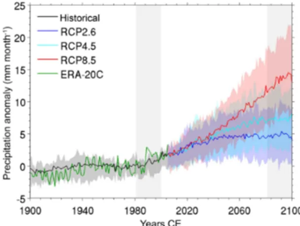
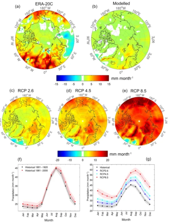
Precipitation data derived from the gridded ERA-20C dataset (Poli et al., 2013) averaged over the whole Arctic (≥ 60◦N) show a positive trend over the last century, with a notable in-crease in the last few decades (Fig. 1), which is in line with previous findings (Serreze et al., 2000; Min et al., 2008). A similar trend is seen in an ensemble of 12 historical CMIP5 simulations (1900–2005; see Table S1 in the Supplement for information on the included models). The spatial pat-tern of precipitation change is heterogeneous across the re-gion (Fig. 2a and b), with the largest increases in annual pre-cipitation over the North Atlantic and Barents Sea and, to a lesser degree, over eastern Asia, western North America, and
Figure 1. Annual precipitation anomaly (relative to the period 1961–1990) of the Arctic (> = 60◦N) derived from ensemble mean of historical (1900–2005) and RCP (2006–2100) simulations us-ing 12 CMIP5 climate models (Taylor et al., 2012). The green line shows the annual precipitation anomaly derived from the ERA-20C reanalysis dataset (Poli et al., 2013). Solid lines represent multi-model ensemble means, while shading around the solid lines repre-sents the interquartile ensemble spreads (25th and 75th quartiles). The vertical light grey shading marks the time period of 1981–2000 (left) and 2081–2100 (right).
the North Pacific (Fig. 2a). Annual precipitation decreased in western Eurasia and locally over eastern Greenland and Sval-bard. The CMIP5 models show a similar pattern, although the increase is much lower and more spatially homogenous (Fig. 2b), with slightly more prominent increases over parts of the North Atlantic and Barents Sea and decreases in areas south-west and south-east of Greenland.
For future hydroclimate projections, 36 CMIP5 simula-tions (12 for each of the Representative Concentration Path-ways: RCP 2.6, RCP 4.5, and RCP 8.5 scenarios) for the period 2006–2100 were used. Multi-model ensemble means represent robust projections of the temporal variation, spatial patterns, and seasonal cycle of the historical and future an-nual precipitation variability over the Arctic region. Simula-tions with all RCPs indicate an increase in mean annual pre-cipitation in the coming century, ranging from 4 mm (RCP 2.6 ensemble mean) to 14 mm (RCP 8.5 ensemble mean; Fig. 1). To obtain the spatial pattern of annual precipita-tion changes, the spatial pattern changes were first calcu-lated based on individual model simulations and then re-gridded to the same spatial resolution as the GFDL-CM3 model (i.e. 144 longitudinal grid cells × 90 latitudinal grid cells). The re-gridded spatial pattern changes based on the individual model simulations were then averaged to create a multi-model ensemble mean.
The most prominent increases in annual precipitation will occur over the Barents Sea, western Scandinavia, eastern Eurasia, and western North America, with decreased precip-itation over the central parts of the North Atlantic (Fig. 2c to e). Moreover, the model simulations suggest an intensified
precipitation cycle with increases in all months, but more prominently outside late spring–early summer (Fig. 2f and g).
2.2 Impacts of Arctic hydroclimate change 2.2.1 Impacts on Arctic environments
Changes in hydroclimate will have impacts on Arctic terres-trial and marine environments, including the cryosphere and the Arctic Ocean (ACIA, 2005). Observational studies show evidence of increased precipitation and river discharge in the Arctic, and hence a freshening of the Arctic Ocean, over the last decades (e.g. Peterson et al., 2006; Min et al., 2008). The freshening will have impacts on ocean convection in the sub-arctic seas, influencing the thermohaline circulation (THC, see below; Min et al., 2008). Increased ocean freshening will also have implications for marine flora and fauna distribu-tion due to altered light and nutrient condidistribu-tions (Carmack et al., 2016). Planktonic primary producers are likely to be affected, some positively and some negatively, and these im-pacts may cascade up the food web and alter the whole ma-rine ecosystem structure (Li et al., 2009), thereby affecting marine biodiversity. Overall, changes in landscape and bio-physical properties, biogeochemical cycling, and chemical transport associated with warmer and wetter conditions will influence ecosystem productivity (e.g. Wrona et al., 2016). Impacts on ecosystems will also affect the Arctic’s indige-nous populations, e.g. through increased risks to infrastruc-ture and water resource planning (Bring et al., 2016), health (Geer et al., 2008), and subsistence-based livelihoods (Ford et al., 2014). As an example of the latter, increased occur-rences of rain events during the cold season, causing the formation of ground ice and preventing winter grazing, will have negative impacts on herbivores, such as reindeer (Stien et al., 2012).
2.2.2 Remote impacts
In general, snow cover in the pan-Arctic region has decreased over the last several decades (Screen and Simmonds, 2012; Shi et al., 2013), although for snow on sea ice knowledge is limited due to the effects of regional variability and a lack of direct observations. This has been attributed to elevated temperatures and an increasing fraction of rain relative to snow, but also to the effects of increasing evaporation from the ocean due to the receding sea ice pack (Bintanja and Sel-ten, 2014). In addition to the local effects described above, changes in snow cover, especially during autumn–winter, af-fect the atmospheric circulation, and this can have remote impacts on the hydroclimate of lower latitudes. For exam-ple, Cohen et al. (2012) suggested that a warmer and wet-ter Arctic atmosphere during autumn, caused by decreasing sea ice coverage, regionally favours increased snow cover in the same season, which dynamically forces negative Arctic Oscillation (AO) conditions in the subsequent winter. The
Figure 2.Simulated and observed Arctic precipitation. Upper panels: (a) observed and (b) modelled changes in annual precipitation over the Arctic region (> = 60◦N) relative to the reference period 1901–1920 and averaged over the 1981–2000 period. The observed pattern is obtained from the ERA-20C reanalysis dataset (Poli et al., 2013). The modelled pattern is derived from ensemble mean of historical (1900– 2005) simulations performed by 12 CMIP5 climate models (Taylor et al., 2012). Middle panels: multi-model (12 CMIP5 models) average changes in annual precipitation relative to the reference period 1981–2000 averaged over the period 2081–2100 under RCP 2.6 (c), RCP 4.5 (d), and RCP 8.5 (e) forcing scenarios. Lower panels: multi-model (12 CMIP5 models) average of seasonal cycle of precipitation over the Arctic (> = 60◦N) for the periods of 1901–1920 (black) and 1981–2000 (red) (f), and for 1981–2000 (black) and 2081–2100 (other colours) (g). Solid lines represent multi-model ensemble means, while shading around the solid lines represents uncertainties expressed as ±2 standard deviations of the mean monthly precipitation over a 20-year period.
negative phase of the AO is associated with a more merid-ional flow of the jet stream, which allows cold Arctic air to penetrate into lower latitudes, occasionally yielding extreme weather events (Overland et al., 2016).
A distinct decline in sea ice extent and thickness has been observed in the past decades (Stroeve et al., 2012; Kwok and Cunningham, 2015). The melting of Arctic sea ice has lo-cal influences, but recent research suggests that it may also have remote impacts on mid-latitudes by perturbing local
energy fluxes at the surface and modifying the atmospheric and oceanic circulation (e.g. Budikova, 2009; Francis et al., 2009). Variations in Arctic sea ice extent influences the North Atlantic Oscillation (NAO; Pedersen et al., 2016), which has a strong influence on precipitation in the North Atlantic re-gion (Hurrell, 1995; Folland et al., 2009). Wu et al. (2013) suggested that winter Arctic sea ice concentration may be a precursor for summer rainfall anomalies over northern Eura-sia and Guo et al. (2014) noted a link between spring Arctic sea ice conditions and the summer monsoon circulation over eastern Asia. On the other hand, it is also likely that lower-latitude phenomena influence Arctic sea ice conditions. For example, wintertime sea ice loss has been linked to different phases of the Pacific Decadal Oscillation (PDO; Screen and Francis, 2016).
Enhanced precipitation and melting of the cryosphere in-creases the run-off from the pan-Arctic land areas and lowers the salinity of the Arctic Ocean, and this will likely have sig-nificant impacts at a local and potentially global scale (Ser-reze and Barry, 2011; Rhein et al., 2013; Carmack et al., 2016). Since the density of the water in the Arctic Ocean determines the location of the thermocline and haloclines, changes in salinity may influence the distribution patterns of organisms and biogeochemical properties (Aagard and Car-mack, 1989; Carmack et al., 2016). Moreover, salinity regu-lates the density of the water in the Arctic Ocean, and through outflow of Arctic water into the North Atlantic it can impact regions at lower latitudes, e.g. by affecting deep water for-mation in the Greenland–Norwegian and Labrador seas and thus the strength of the THC (Aagard and Carmack, 1989; Rahmstorf, 1995; Slater et al., 2007). A disruption of the THC could have global impacts (Vellinga and Wood, 2002). Density also determines the location of the thermoclines and haloclines so that salinity shifts greatly the influence distri-bution of organisms (Aagard and Carmack, 1989; Carmack et al., 2016).
3 Hydroclimate archives and proxies in the Arctic While most archives and proxies that are widely used else-where to infer past climate variability can be found in the Arctic, their application require specific treatment and inter-pretation. The following section describes and discusses the characteristics and the limitations of these in the Arctic envi-ronment.
3.1 Lake sediments: varves and biomarkers 3.1.1 Arctic lakes
Most lakes in the Arctic were formed just after local retreats of ice sheets, glaciers, and ice caps after the last glaciation; hence, their ages and the potential lengths of the records they contain range from the entire Holocene in Beringia and Scan-dinavia to only a few hundred years in Greenland or Iceland.
The last 2000 years has, in general, been characterised by minor glacier fluctuations prior to the general melt of the re-cent decades (Solomina et al., 2016). This relative stability in surface area over the last 2 millennia makes lakes excellent recorders of hydroclimate variability for this period. What makes the lakes different in the Arctic is the very strong sea-sonality that is reflected in a long to very long ice cover pe-riod. A long ice cover season substantially reduces the in-put of particles from the watershed to the lake, frequently to an unmeasurable quantity. Therefore, what is recorded in Arctic lacustrine sediments is strongly biased towards the ice-free periods, i.e. spring snowmelt, short summer, and early autumn. Another characteristic of the Arctic is phys-ical weathering related to gelifaction and sparse vegetation cover, making large quantities of easily eroded minerogenic matter available to be transported into lakes (Zolitschka et al., 2015).
Lake systems in the Arctic differ depending on the pres-ence or abspres-ence of glaciers in their watershed. Snow-fed wa-tersheds experience maximum discharge during snowmelt in spring. They become depleted in water once the snow cover has melted, reducing sediment transport in the latter part of the ice-free season. On the other hand, glacierised watersheds are not water limited; i.e. the water supply to the lake trib-utary can last the entire summer and autumn until tempera-tures decrease below zero. Discharge, and therefore sediment transport, is usually driven by temperature at the elevation of the glacier and is usually at a maximum during summer. In addition, lake systems in glacierised watersheds may on rare occasions be subjected to catastrophic floods (called Jökulh-laups), which are due to collapsing ice dams retaining vast amounts of water in intra- or supra-glacial lakes, and result-ing in high sediment fluxes to the lakes.
Many watersheds in the Arctic are also affected by the presence of permafrost. During summer, the permafrost thaws in its upper part (active layer), leaving sediment eas-ily mobilised by small amounts of rainfall. This increases the risk of slope detachments and can result in debris flows or very high sediment yields in lake tributaries (Lewis et al., 2005). The presence of permafrost also makes the dating of lacustrine sediments difficult because organic matter can be stored in the soils for a long period prior to being transported to the lakes (Abbott and Stafford Jr., 1996).
In the high Arctic, sources of organic matter in lake sed-iments are both allochthonous and autochthonous, i.e. pro-duced in the watershed or the lake. The relative contribution of these sources may in part be controlled by climate (Out-ridge et al., 2017), although the allochthonous organic matter remains dominant, and the total amount preserved remains low (Abbott and Stafford Jr., 1996; Gälman et al., 2008). Conversely, lakes located in the southernmost part of the Arctic, such as in the boreal forests of Scandinavia or North America, experience a season with higher primary productiv-ity. Their total organic carbon content can be relatively high
(Gälman et al., 2008) when anoxic conditions at the bottom of the water column prevail, slowing down its degradation.
3.1.2 Extracting hydroclimatic information from Arctic lakes
Most of the proxies used elsewhere in the world for the pur-pose of reconstructing past hydroclimate can also be anal-ysed in Arctic lakes. Extensive experience has enabled their use in the Arctic in spite of the harsh nature of the environ-ment.
Pollen. Pollen can successfully be used to reconstruct pre-cipitation because the response of plants to moisture changes is direct and well studied. Although a substantial propor-tion of the pollen in the high Arctic arrives from forested regions to the south, pollen assemblages can still be used to reconstruct the local conditions (e.g. Gajewski, 2002, 2006, 2015b). The sediments may be contaminated by older pollen stored in the soils or, in some cases, from Tertiary deposits in the watershed (Gajewski et al., 1995). Nevertheless, an-nual precipitation has been reconstructed, along with temper-ature (Gajewski, 2015a), using pollen assemblages and are presented in Sect. 4.2.
Chironomids. In the Arctic, chironomids are primarily affected by lake depths, temperature and water chemistry (Gajewski et al., 2005). Provided that changes in precipita-tion regime affect the depth of a lake and the pH or nutri-ent supply, chironomids can be used (Medeiros et al., 2015). However, most work has emphasised the reconstruction of temperature, and there would need to be relatively large changes in depth to have a noticeable effect on the chirono-mid community (e.g. Barley et al., 2006; Fortin et al., 2015). Diatoms. These can presumably be used to reconstruct past moisture through various indirect methods. The primary control on diatoms is pH (Finkelstein et al., 2014), and to the extent this is affected by lake level variations, it could be used as an indirect proxy. Lake level changes affecting the relative area of deep and shallow water can be registered by diatoms; these have been used in other regions but not in the Arctic. A study of stable oxygen isotopes in diatom frustules allowed for a palaeohydrological reconstruction from Baffin Island, Canada (Chapligin et al., 2016).
Hydrogen isotopes and biomarkers. The source of envi-ronmental water in terrestrial systems is precipitation. Pre-cipitation δD values are influenced by the location, tempera-ture, and relative humidity of the primary evaporation source of the moisture, the air mass trajectory, and the temperature at condensation (Dansgaard, 1964; Boyle, 1997; Pierrehum-bert, 1999; Masson-Delmotte et al., 2008; Frankenberg et al., 2009; Theakstone, 2011; Sjolte et al., 2014). Evaporative en-richment can cause environmental water, including lake wa-ter, soil moisture, and leaf wawa-ter, to become D-enriched rel-ative to the original precipitation. Thus, lake-sediment-based lipid δD records can provide important insights into the vari-ability of both precipitation δD values and evaporative
en-richment and thus ultimately into local hydrological changes. There are only a handful of published studies using δD values of leaf waxes and algal lipids to reconstruct past hydrological changes in the Arctic (Thomas et al., 2012, 2016; Balascio et al., 2013, 2017; Moossen et al., 2015; Keisling et al., 2017). The palaeohydrological interpretations of these δD records differ among the studies, reflecting the fact that different lake catchments respond differently to hydrologic changes (and over different timescales), but also highlights our in-complete understanding of the biological and environmental factors that influence hydrogen isotope variability in lipids. Palaeohydrologic interpretations are better constrained when lipids with δD values representing lake water (e.g. those de-rived from algae and macrophytes) are considered together with those representing leaf water (e.g. long-chain n-alkanes and long-chain n-alkanoic acids; Balascio et al., 2013, 2017; Rach et al., 2014; Muschitiello et al., 2015; Thomas et al., 2016). Together, δD values of these compounds can be used to quantify isotopic differences between lake water and leaf water, which can reveal changes in the duration of summer ice cover (Balascio et al., 2013), seasonality of precipitation (Thomas et al., 2016), or the vegetation type contributing lipids to the lake sediments (Balascio et al., 2017). Rach et al. (2017) propose an approach using paired terrestrial and aquatic lipid δD values and plant physiological models to quantitatively reconstruct relative humidity changes through time. This approach may prove effective in some Arctic set-tings.
Several physical and geochemical proxies have been used to infer past hydrology. Mass accumulation rate (MAR) is a measure of the amount of sediment accumulated at the bottom of the lake (e.g. Weltje, 2012). It is usually directly linked to the lake tributary discharge in lakes with low pri-mary productivity (Petterson et al., 1999). Obtaining MAR requires an accurate age model and measurements of density. Density, magnetic susceptibility, and elemental composition are all indicators of the detrital input, which is again linked to the lake tributary discharge (Petterson et al., 1999; Dearing et al., 2001; Cuven et al., 2010). The grain size of the terrige-nous fraction is an indicator of the competence of the flow (maximum discharge), its duration, and physical processes occurring in the lake water column (Lapointe et al., 2012). Together, these physical and geochemical proxies are rarely used in Arctic sedimentary sequences with massive structure because of the complexity of their interpretation; however, they have proven to be useful tools in annually laminated sediments.
3.1.3 Varved sediments
Varved sediments are difficult to find and probably rarely de-posited (Zolitschka et al., 2015). However, several lakes with varved sediments have been found in the Arctic, probably because the very strong seasonal contrast in sediment sup-ply favours the formation of varves. Lakes containing varves
tend to be deep enough to prevent bioturbation and are usu-ally found in watersheds with high sediment yield. As such, many of the varved records cannot be directly compared to lakes used in diatom and pollen studies because the latter are usually studied in smaller systems. The advantages of varved sediments are that they contain their own chronol-ogy, that annual fluxes can be measured through the mea-surement of density, and that their properties can be cal-ibrated against instrumental records (Hardy et al., 1996). In the Arctic, two types of varves exist: clastic varves and mixed clastic–biogenic varves, as discussed in Zolitshcka et al. (2015).
Clastic varves
Clastic varves result from the complex interactions between sediment availability (geomorphological control), seasonal run-off variations carrying suspended sediment (hydrocli-matic control), the thermal density structure of the lake wa-ter column, and the bathymetry of the lake (limnological control). These varves are typically composed of a coarse-grained lower lamina that grades into a fine-coarse-grained upper lamina (e.g. Lake DV09; Courtney-Mustaphi and Gajewski, 2013; Lake C2; Zolitschka, 1996). Additional coarse-grained laminae can be deposited and can be related to multiple pulses of snowmelt or rain events (Ringberg and Erlström, 1999; Cockburn and Lamoureux, 2008). The finest clay frac-tion remains in the water column and is only deposited un-der quiet conditions during the following winter (Francus et al., 2008). Therefore, the presence of a distinct clay cap is the main criteria for identifying a year of sedimentation (Zolitschka et al., 2015).
Several individual parameters can be measured from each varve sequence: total thickness, sublamina thickness, den-sity, mass accumulation rate, total and sublamina grain size, elemental composition, and magnetic susceptibility. Linking these properties with hydroclimate conditions requires mon-itoring the processes occurring in the watershed and the lake, with each system being different. Disentangling the respec-tive effect of the temperature from moisture is a challenge due in part to the difficulty in obtaining data for calibra-tion in the Arctic. When comparing varve properties to ob-servational climate data, they often contain signals of both temperature and precipitation (e.g. Table 2 of Cuven et al., 2011; Lamoureux and Gilbert, 2004), although the temper-ature signal has been reported more often in the litertemper-ature. However, this may be because more robust measurements of instrumental temperature are available compared to precip-itation (especially snow) and precipprecip-itation patterns tends to be more variable over a region, making correlation with sed-iment properties more difficult.
Despite these difficulties, several authors reported correla-tions of varve sequence data with hydroclimate. In general, the hydroclimate is revealed in the measurement of a specific part of the sedimentary cycle, and not by a parameter that
integrates the whole year of sedimentation such as the total varve thickness. For instance, Lapointe et al. (2012) showed a correlation (r = 0.85, p = 0.0001) between the largest rain-fall events and the coarsest grain-size fraction of each varve. Lamoureux et al. (2006) found a correlation between varve thickness of Sanagak Lake, Boothia Peninsula and snow-water equivalent in the snow-watershed, but they were unable to calibrate the series due to lack of calibration data. Francus et al. (2002) found a correlation (r = 0.53, p < 0.05) be-tween snowmelt intensity and the median grain size. Lam-oureux (2000) found an association of sediment yield esti-mates of Nicolay Lake, Cornwallis Island and rainfall events.
Mixed (clastic–biogenic) varves
In less harsh environments, such as in central Scandinavia, the vegetation of the catchment area and soils is more devel-oped, allowing decaying organic matter to be incorporated into the lacustrine system. At the same time, the primary pro-ductivity in the water column during the warmer seasons is large enough to be recorded in the sedimentary archive. This results in the accumulation of a mixed type known as clastic– biogenic (or clastic–organic) varves. These typically contain a characteristic minerogenic lamina, usually showing graded bedding that is directly related to the duration and strength of the spring flood (e.g. Ojala et al., 2000; Snowball et al., 2002; Tiljander et al., 2003) and a biogenic lamina that can be composed of autochthonous organic matter (e.g. diatom frustules) and/or allochthonous organic debris.
Proxies measured with annual resolution on these mixed varves include (1) total varve thickness, (2) growing sea-son lamina (GSL) thickness, (3) winter lamina (WL) thick-ness (Saarni et al., 2015), and (4) relative X-ray densitometry (Ojala and Francus, 2002). Correlations with climate param-eters vary from site to site and sometimes through time at a single site (Saarni et al., 2015). Only a small number of lacus-trine sequences, all of them from Scandinavia, have been suc-cessfully correlated with precipitation or moisture. At Lake Nautajärvi annual and winter precipitation was reconstructed using relative X-ray densitometry (Ojala and Alenius, 2005), whereas at Lake Kallio-Kourujärvi, the growing season lam-ina was linked to annual precipitation (Saarni et al., 2015). Rydberg and Martinez-Cortizas (2014) showed that high ac-cumulation of snow resulted in high mineral matter content, and Wohlfarth et al. (1998) found a significant correlation between early spring–summer precipitation and total varve thickness in north-central Sweden.
As with clastic varves, it is quite difficult to separate the temperature from the moisture signal. Ojala and Ale-nius (2005) showed that direct annual and seasonal com-parisons between raw varve data and instrumental measure-ments are complicated. Itkonen and Salonen (1994) showed that total varve thickness of three Finnish lakes were cor-related with both temperature and precipitation, the correla-tion being weaker for precipitacorrela-tion. Nevertheless, sediment
trap studies clearly but qualitatively showed the sensitivity of such systems to varying hydroclimate conditions (Ojala et al., 2013; Rydberg and Martinez-Cortizas, 2014).
3.2 Peat deposits
3.2.1 Peatland processes and peat archive
Peatlands are wetland ecosystems that preserve their devel-opmental history over millennia. Peat deposits are products of the balance between plant production and organic mat-ter decomposition (Clymo, 1984), and both processes are af-fected by climate. As a result, peat accumulation is inherently influenced by autogenic–ecological and allogenic–climatic factors, as well as their interactions (Belyea and Baird, 2006). Many peat-based proxies (see below) have been used to reconstruct peatland hydrology and water table dynamics, likely connected with regional hydroclimate. This ability of wetland communities to record hydrological change results largely from their occurrence in environments where a single extremely variable habitat factor, i.e. water supply, is pre-dominant (Tallis, 1983). However, empirical and modelling studies show the importance of autogenic process and eco-hydrological feedbacks (e.g. Tuittila et al., 2007; Swindles et al., 2012; Loisel and Yu, 2013; Väliranta et al., 2016). Clearly, consideration of biological processes and ecological feedbacks is needed when using these systems for climate reconstructions.
Peatland plants shape their own habitat since they form their own growth substrate: peat. Hence, peatlands are capa-ble of recording in their deposits the effects of past vegeta-tional and ecological changes. Within the peat lies a repos-itory of botanical, zoological, environmental, and biogeo-chemical information, which is important for understanding past climatic conditions. These palaeorecords are used to es-timate the rates of peat formation or degradation, past veg-etation, climatic conditions, and depositional environments (Moore and Shearer, 1997; Blackford, 2000). Analysis of peat deposits has undergone major developments during the last several decades regarding coring techniques, peat sam-pling and analysis, geochronology, identification of plant re-mains and other microfossils, and quantitative multivariate techniques (e.g. Barber et al., 1994, 1998; Väliranta et al., 2007; Charman et al., 2009; Chambers et al., 2011; Mathi-jssen et al., 2016, 2017).
Stratigraphic studies in peatlands have shown a hydroseral succession in which wet swamp and fen communities grad-ually develop into dry bog communities (Tallis, 1983; Ko-rhola, 1992; Väliranta et al., 2016). These changes are largely autogenic, connected to the growth of wetland communi-ties, and caused by climatic variability or artificial drainage. Hilbert et al. (2000) developed a model of peatland growth that explicitly incorporates hydrology and feedbacks be-tween moisture storage and peatland production and de-composition. They suggest that drier ombrotrophic peatlands
(most bogs) will adjust relatively quickly to perturbations in moisture storage, while wetter ombrotrophic peatlands (mineral-rich fens) are relatively unstable and can withstand only very small changes in water tables (Mathijssen et al., 2014). Climate change will affect the hydrology of individ-ual peatland ecosystems mainly through changes in precipi-tation and temperature. As the hydrology of the surface layer of a bog is dependent on atmospheric inputs (Ingram, 1983), changes in the ratio of precipitation to evapotranspiration may be expected to be the main factor driving ecosystem change. In particular, ombrotrophic peatlands are regarded as directly coupled to the atmosphere through precipitation and hydrology change (Barber et al., 1994) such that their wa-ter levels and dominant plants will reflect the prevailing cli-mate. More specifically, their water table variability has been shown to be highly correlated with the total summer seasonal moisture deficit (precipitation–evapotranspiration; Charman, 2007).
Modern investigations of past climate are performed with an emphasis on obtaining the highest possible time resolution for a given archive. Radiocarbon dating is one of the main methods used to establish peat chronologies. The best ma-terials for ensuring accurate dates are aboveground remains of plants that assimilated atmospheric CO2, e.g. short-lived
plant macrofossils and pollen whose14C age is consequently not affected by an old carbon effect. Suitable materials for sample selection are Sphagnum mosses (branches, stems, and leaves) or, if not present, aboveground leaves and stems of dwarf shrubs (e.g. Nilsson et al., 2001; see however Väliranta et al., 2014). Age–depth models that are considered ecolog-ically plausible and that take into account likely modes of peat accumulation include (1) linear accumulation, (2) con-cave curves (caused by continuing decomposition of fossil matter in the peat deposit; Yu et al., 2001), (3) convex curves (with deposits slowing their accumulation when approach-ing a height limit; Belyea and Baird, 2006), and (4) Bayesian models that can include prior information on stratigraphy, ac-cumulation rate and variability, and/or detect outlying dates (reviewed by Parnell et al., 2011). The robustness of age models can be significantly improved and the uncertainties reduced by using multiple dating methods on a single core. Most commonly, the uppermost layer can be dated using at-mospheric fall-out radionuclides (e.g. 210Pb; see Le Roux and Marshall, 2011) and spheroidal carbonaceous particle (SCP) profiles (Yang et al., 2001), while tephrostratigraphy can potentially be applied throughout the core (Swindles et al., 2010). With suitable statistical treatment, all results can be combined into one reliable chronology which provides the backbone for interpretations of palaeoclimatic and palaeoen-vironmental change data.
3.2.2 Peat-based hydroclimate proxies
Peatland formation can initiate via three processes: primary peatland formation, terrestrialisation, or paludification
(Ry-din and Jeglum, 2006). In primary peatland formation, peat is formed directly on wet mineral soil when the land is newly exposed due to crustal uplift or deglaciation, whereas in terrestrialisation and paludification the area colonised by peatland vegetation has experienced previous sediment de-position or soil development (e.g. Tuittila et al., 2013). In-formation on hydroclimatic conditions can be derived from these processes, especially when the different peat formation types show systematic and isochronic patterns over wide ge-ographic areas. For example, in paludification, the prereq-uisite is that the local hydrological conditions become wet-ter, for instance induced by climatic change, fire, or beaver damming, resulting in waterlogged soil conditions that pro-mote peat accumulation (Charman, 2002; Gorham et al., 2007; Rydin and Jeglum, 2006). A new conceptual model of episodic, drought-triggered terrestrialisation presents in-filling as an allogenic process driven by decadal to multi-decadal hydroclimatic variability (Ireland et al., 2012).
Recently, Ruppel et al. (2013) presented a comprehensive account of postglacial peatland formation histories in North America and northern Europe using a dataset of 1400 basal peat ages accompanied by below-peat sediment-type inter-pretations. Their data, mainly focusing on boreal–Arctic re-gions, indicates that peat formation processes exhibited some clear spatiotemporal patterns. Unfortunately, the overwhelm-ing majority of the basal peat accounts originate from the deepest and often the oldest parts of peatlands, and there-fore the last 2 millennia are clearly under-represented in the present data. However, existing studies illustrate the poten-tial of using peat initiation and expansion data to account for changes in regional moisture regimes, also in more recent times. The formation of new peatland areas does not nec-essarily decrease when the initiation rates decrease, but new peatland areas are continuously formed via lateral expansion. Peat bulk density (or organic matter density) in down-core profiles has been used to reflect overall peat decom-position, which in many peatland regions is controlled by surface moisture and hydroclimate conditions (e.g. Yu et al., 2003). The rationale is that well-preserved peat is loose and has low organic matter density, most likely deposited under wet conditions promoting the protection of organic matter in an anaerobic environment. Peat bulk density values are typi-cally 0.05 to 0.2 g cm−3in high-latitude regions (Chamber et al., 2011). Peat humification is another proxy for the degree of peat decomposition which can be estimated or measured in the field or laboratory using a range of methods (Cham-ber et al., 2011). Humification can be used as a proxy for peatland surface wetness, as moisture is a key determinant of decomposition, and regional hydroclimate in the Arctic (e.g. Borgmark, 2005; Borgmark and Wastegård, 2008; Vorren et al., 2012).
Net carbon accumulation is the balance between produc-tion and decomposiproduc-tion, both of which are influenced directly or indirectly by climate (Yu et al., 2009). However, recent syntheses indicate that temperature-driven production might
be more important than moisture-controlled decomposition in determining net peat accumulation (e.g. Beilman et al., 2009; Charman et al., 2013). Therefore, without constraints from other proxies, it is difficult to infer hydroclimate from peat accumulation records (Mathijssen et al., 2016, 2017). As mosses are the dominant plants in peatlands, carbon iso-topes from these mosses are useful for inferring peatland moisture conditions. In wet conditions, water films around moss leaves will reduce the conductance of pores on the leaf surface to CO2uptake, reducing discrimination against13C
and resulting in high carbon isotope values (Rice, 2000). Car-bon isotopes have been shown to reflect surface moisture in peatlands (e.g. Loisel et al., 2009). In addition, Nichols et al. (2009) used compound-specific carbon and hydrogen iso-topes from peatlands in the Arctic to evaluate summer sur-face wetness and precipitation seasonality.
Because plant macrofossils reflect changing abundances of climatically sensitive peatland vegetation, they have been used not only for reconstructing the local vegetation history of peatlands but also for inferring past peatland hydrolog-ical changes and, by extension, regional climate variability (e.g. Barber et al., 1998; Hughes et al., 2000; Swindles et al., 2007; Väliranta et al., 2007; Mauquoy et al., 2008; Math-ijssen et al., 2014, 2016, 2017). Traditionally, plant-based peatland surface wetness reconstructions have been qualita-tive or semi-quantitaqualita-tive based on the identification of phases of relatively low local water tables (showing increased rep-resentation of hummock species) and phases of higher local water table depths (lawn and hollow species; Mauquoy et al., 2002; Pancost et al., 2002; Sillasoo et al., 2007). More re-cently, ordination techniques (e.g. PCA and DCA) have been used to create a single index of peatland surface wetness based on the total subfossil dataset for a peat profile (Bar-ber et al., 1994; Mauquoy et al., 2004; Sillasoo et al., 2007; Zhang et al., 2017) in which it is assumed that the principal axis of variability in the dataset is linked to hydrology. The most recent progress in identification and quantification tech-niques of plant macrofossils (e.g. the Quadrat Leaf Count method; Mauquoy et al., 2010), together with careful cali-bration with modern plant community data, allows for the quantification of past peatland water table fluctuations with great accuracy. Väliranta et al. (2007) developed a transfer function by calibrating plant macrofossil records against the modern vegetation–water table relationship in order to quan-titatively reconstruct peatland surface wetness trends for the late Holocene. The inferred water tables showed strong fluc-tuations, with an overall amplitude of ca. 40 cm. During the last 2 millennia, they found generally dry conditions until ca. 1600 cal BP (ca. 400 CE), varying water tables during the following 4 centuries, and dry conditions from ca. 1200 to 700 cal BP (ca. 800–1300 CE, covering the MCA). The sub-sequent centuries were again variable, while the period 500– 200 cal BP (1500–1800 CE, covering the LIA) was wet and the last 2 centuries dry except for the very recent years. The comparison of water table reconstructions based on
macro-fossils and testate amoebae at two bogs in Estonia and Fin-land increased the confidence in using bog plants in quanti-tative hydrological reconstructions (Väliranta et al., 2011).
Testate amoebae (Protozoa: Rhizopoda) are unicellular an-imals with distinct environmental preferences which live in abundance on the surface of most peat bogs. These amoeboid protozoans produce morphologically distinct shells, which are commonly used as surface moisture proxies in peat-based palaeoclimate studies (Mitchell et al., 2008). Although the moisture sensitivity of these organisms has been known for a long time, work over the past several decades has demon-strated the utility of testate amoebae as quantitative peat-land surface moisture indicators. Their indicator value in documenting surface moisture variation has been demon-strated by coherence in reconstructions of wet and dry fluc-tuations within and between peatland sites (Hendon et al., 2001; Booth et al., 2006). A protocol of their use in palaeo-hydrological studies is provided by Charman et al. (2000) and Booth et al. (2010). Testate amoebae have been used for tracing hydrological changes in temperate peatlands in sev-eral regions of the world, as well as in the boreal and subarc-tic peatlands of Canada and the US (Payne et al., 2006; Loisel and Garneau, 2010; van Bellen et al., 2011; Bunbury et al., 2012; Lamarre et al., 2012, 2013). In addition to bogs, they can also be applied in fens (Payne, 2011). Recently, Swin-dles et al. (2015) and Zhang et al. (2017, 2018) tested the potential of testate amoebae for peatland palaeohydrologi-cal reconstruction in permafrost peatlands based on sites in Arctic Sweden and Russia, respectively. These evaluations confirmed that water table depth and moisture content are the dominant controls on the distribution of testate amoe-bae in Arctic peatlands, corroborating the results from stud-ies in mid-latitude regions. New testate-amoeba-based wa-ter table transfer functions were created with good predic-tive powers and the transfer functions were applied to short cores from permafrost peatlands. All records revealed a ma-jor shift in peatland hydrology, which in one case coincided with the onset of the Little Ice Age (Swindles et al., 2015). The new modern training sets will enable palaeohydrologi-cal reconstruction from permafrost peatlands in Northern Eu-rope, thereby permitting a greatly improved understanding of the long-term hydrological dynamics of these ecosystems and the general variability in hydroclimatic conditions.
3.3 Tree-ring data
Distinct, precisely dateable tree rings are generally formed in areas with pronounced seasonality, which results in a single period of cambial activity (growth) and dormancy per cal-endar year. The width, density, and isotopic compositions of a tree ring are partly determined by local weather and cli-mate, and the closer to the ecological limit of distribution a tree grows, the more sensitive to climate it will be. Due to the large spatial distribution of trees across extra-tropical re-gions, their capacity to live for many years and their potential
for developing precise, annually resolved chronologies, tree-ring data have been widely used to infer late Holocene varia-tions in a range of climate parameters on local to hemispheric scales.
3.3.1 Tree-ring width and density
Measurements of annual tree-ring width (TRW) are per-haps the most important data source for quantitative esti-mates of high- to low-frequency climate variability during the past centuries to millennia. The advantage of TRW comes from its annual resolution and a comprehensible understand-ing of the climatic controls on the tree-runderstand-ing growth dynam-ics (e.g. Vaganov et al., 2006). Tree rings have the advan-tage of numerical calibration, verification, and the poten-tial to capture seasonal extreme events not possible using lower-resolution, less temporally well-constrained archives. The tree-ring community has generated an expansive net-work of TRW chronologies covering a wide range of species and ecosystems across the globe, including the boreal–Arctic ecotone. In general, trees growing close to their latitudinal or altitudinal limit of distribution will be sensitive to warm-season temperature, while trees growing in semi-arid to arid regions are limited by precipitation and moisture (St George, 2014; St George and Ault, 2014; Hellman et al., 2016). Con-sequently, most but not all high-latitude TRW chronologies exhibit strong positive associations with summer tempera-ture and only weak correlations with summer or winter rain-fall. Tree-ring data from the high northern latitudes have been used in several reconstructions of Northern Hemisphere temperature (e.g. D’Arrigo and Jacoby, 1993; Jones et al., 1998; Briffa et al., 2001; Esper et al., 2002; D’Arrigo et al., 2006; Schneider et al., 2015; Stoffel et al., 2015; Wilson et al., 2016) and reconstructions targeting Arctic tempera-tures (Overpeck et al., 1997; Kaufman et al., 2009; Shi et al., 2012; Hanhijärvi et al., 2013; McKay and Kaufman, 2014). The few chronologies in the cool boreal and Arctic regions developed from precipitation-sensitive trees are mainly lo-cated in continental climate zones, such as western Canada, Alaska, and eastern Fennoscandia (see Fig. 1 in St George and Ault, 2014). Many TRW records are negatively corre-lated with summer rainfall, and most of these are found in the colder high-latitude regions. Positive correlations with prior-summer precipitation are also common across the Arc-tic. This carry-over effect may be caused by increased photo-synthetic reserve accumulation in years with sufficient mois-ture supplying resources that can be used for secondary tissue growth in subsequent years. A proportion of this association likely reflects the inverse relationship between summer tem-perature and precipitation observed in these regions.
Although TRW is the most commonly used tree-ring proxy, at high latitudes, wood densitometric measurements, specifically maximum latewood density (MXD) and its sur-rogate blue intensity (BI), are commonly being viewed as superior temperature proxies compared to TRW. It would
seem that the strong correlation between MXD–BI and tem-perature would prevent their use in hydroclimate reconstruc-tions. However, recent studies (Cook et al., 2015; Seftigen et al., 2015a, b) have indirectly used high-latitude temperature-sensitive tree-ring data to reconstruct soil moisture availabil-ity by considering the inverse relationship between available soil moisture and clear skies, higher temperatures, increased evaporation, and reduced rainfall. Thus, the negative corre-lation between the high-latitude tree-ring data and drought metrics, such as the self-calibrating Palmer Drought Sever-ity Index (scPDSI; van der Schrier et al., 2006a, b) and the Standardised Precipitation Evapotranspiration Index (SPEI; Vicente-Serrano et al., 2010), can be used to generate recon-structions that are comparable to those from arid and semi-arid regions where tree growth is strongly limited by rainfall. Many high-latitude MXD data that are mainly influenced by temperature also exhibit a negative, albeit weak, statistical association with summer precipitation (Briffa et al., 2002). This mixed response explains why such data have success-fully been used in reconstructions of drought indices that in-tegrate both temperature and precipitation.
3.3.2 Stable isotopes in tree rings
The isotopic ratios of wood, lignin, and tree-ring cellulose are influenced by a different and more limited range of envi-ronmental and physiological controls than TRW and MXD. For this reason, stable isotopes in tree rings provide addi-tional palaeoclimate information to support and enhance the information attainable from the physical proxies (McCarroll and Loader, 2004; Gessler et al., 2014). Similar to TRW and MXD, the strength and relative expression of these climatic controls will vary geographically and to a degree with lo-cal edaphic conditions and tree species. In simple terms, car-bon isotopic variability reflects changes in the balance be-tween the conductance of carbon dioxide (CO2) from the
at-mosphere to the site of photosynthesis and assimilation rate, which are influenced by moisture stress and photosynthet-ically active radiation (PAR), respectively. Temperature and nutrient availability may also contribute to this signal through an influence upon the rate of chemical reaction and produc-tion of photosynthetic enzymes (Farquhar et al., 1982; Schei-degger et al., 2000; Hari and Nöjd, 2009). Oxygen and hy-drogen isotopes are more closely related to the isotopic com-position of the water used by the tree during photosynthesis, which may reflect a combination of moisture sources subse-quently modified by the evaporative enrichment of leaf wa-ter (vapour pressure deficit and relative humidity) and plant physiological processes (Barbour et al., 2001; Danis et al., 2006; Treydte et al., 2014; Roden et al., 2000).
Since the earliest isotopic dendroclimatology studies con-ducted in the Arctic (Sonninen and Jungner, 1995; McCar-roll and Pawellek, 1998; Waterhouse et al., 2000), several studies have made significant contributions to palaeohydrol-ogy (e.g. Waterhouse et al., 2000; Holzkämper et al., 2008,
2012; Sidorova et al., 2008, 2009; Porter et al., 2009). The combination of long-lived trees, robust dendrochronologies and excellent sample preservation both on land and in lakes have facilitated the development of several multi-centennial to millennial length isotopic records (Boettger et al., 2003; Kremenetsky et al., 2004; Sidorova et al., 2008; Young et al., 2010; Gagen et al., 2011; Porter et al., 2014; Loader et al., 2013). However, because moisture is rarely the domi-nant tree-growth-limiting factor across much of the Arctic region, there is a limitation to the hydroclimate informa-tion that can be reconstructed using the isotopic approach. Using a multi-parameter approach, several studies (Loader et al., 2013; Young et al., 2010, 2012; Gagen et al., 2011) provided sunshine–cloud estimates and were able to demon-strate large-scale shifts in the dominance of Arctic and mar-itime air masses over the northern Fennoscandian region dur-ing the LIA and MCA. Such multi-parameter studies are po-tentially very powerful as they help to develop testable hy-potheses relating to the future response of the Arctic atmo-sphere and provide a foundation for developing a circumpo-lar isotope network to track changes in atmospheric circula-tion and its relacircula-tionship to climate throughout the Common Era.
Reconstructions based upon oxygen and hydrogen iso-topes have yet to reveal the same clear and stable corre-lations with instrumental data observed for carbon, but are likely to relate most closely to local and regional hydrocli-mate through their close link with stable isotopes in precipi-tation (Roden et al., 2000). The relative contributions of the isotopic signal from snowmelt and growing season precipi-tation used to form the tree rings is an area requiring inves-tigation. Links between δ18O and both moisture and temper-ature have been identified (Sidorova et al., 2009; Knorre et al., 2010). Further south, Hilasvuori and Berninger (2010) linked oxygen (and carbon isotopes) most strongly to cloud cover, with precipitation, relative humidity, and temperature exhibiting lesser correlations. Hydrogen isotopes did not cor-relate as strongly as oxygen or carbon, with the strongest statistically significant relationships being with precipitation. Seftigen et al. (2011) linked δ18O to precipitation, but noted that this relationship was unstable through time, possibly due to changes in the atmospheric circulation. If the same close relationship observed between water isotope composi-tion and tree-ring cellulose in mid-latitude regions (Danis et al., 2006; Labuhn et al., 2014; Treydte et al., 2014; Young et al., 2015) is confirmed in the Arctic, then the potential ex-ists for developing long records of the isotopic composition of precipitation suitable for large-scale mapping of isotope climate (Hemming et al., 2007; Saurer et al., 2012; Young et al., 2015). Reconstructing the stable isotopic composition of precipitation will likely provide a more useful, more di-rect link to the global hydrological cycle “isotope climate” (Birks and Edwards, 2009; Bowen, 2010) than a statistical calibration of water isotopes developed against a measured
(indirect) meteorological variable which may vary in the de-gree of its control across space or over time.
3.3.3 Tree-ring-based hydroclimate reconstructions Tree-ring data have been used to locally estimate a vari-ety of hydroclimate variables, such as precipitation, drought, streamflow, cloud cover, and snowpack (e.g. Stahle and Cleaveland, 1988; Waterhouse et al., 2000; Pederson et al., 2001; Meko et al., 2001; Woodhouse, 2003; Gray et al., 2003; Young et al., 2010; Gagen et al., 2011). Moreover, networks of tree-ring chronologies have been used to make spatial (or field) hydroclimate reconstructions (Nicault et al., 2007; Cook et al., 1999, 2004, 2010; Fang et al., 2011; Touchan et al., 2011; Hua et al., 2013). However, these studies have al-most exclusively utilised tree-ring data from lower latitudes outside the Arctic region.
Within the Arctic, trees are naturally constrained to exist below the latitudinal treeline, extending as far as ca. 73◦N in parts of central Siberia, and as noted above, the majority of the tree-ring data in the region come from temperature-sensitive trees. Still, with careful site selection, it is pos-sible to find trees that are sensitive to moisture variabil-ity, and a few studies have inferred past precipitation vari-ability using ring-width data. Indeed, a handful of recon-structions of local hydroclimate from the Arctic have been published. These have mainly focused on late spring–early summer precipitation. The longest record, and presently the most widely used high-resolution hydroclimate proxy for high-latitude Fennoscandia, comes from south-eastern Fin-land where Scots pine TRW was used to reconstruct annual May–June precipitation over the last millennium (Helama and Lindholm, 2003). Later an updated chronology from the same region was used to highlight the distinct and persistent “mega-drought” from the early 9th century to the 13th cen-tury CE (Helama et al., 2009). The same parameter was also reconstructed from Scots pine for east-central Sweden back to 1560 CE by Jönsson and Nilsson (2009). In North Amer-ica, Pisaric et al. (2009) reconstructed the June precipitation of the North-west Territories, Canada using a TRW network. The only reconstruction of hydroclimate outside the growing season was presented by Linderholm and Chen (2005), who developed a 400-year-long winter (September–April) precip-itation reconstruction with 5-year resolution based on Scots pine TRW data from west-central Scandinavia.
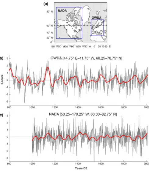
Focusing on hydroclimate field reconstructions, one of the earliest works to use tree rings to reconstruct past moisture variability in a high-latitude region was the North American Drought Atlas (NADA; Fig. 3a). The atlas was first released in 2004 (Cook et al., 2004), then covering the continental US and later updated (Cook et al., 2007) with an expanded tree-ring network to include parts of the Canadian Arctic. Al-though significant portions of the latter region are at present under-represented in NADA, the tree-ring coverage still pro-vides valuable hydroclimate reconstructions for a number of
regions. The summer PDSI reconstruction data for the Arctic part of NADA extend back to the 1000 CE, indicating slightly drier conditions during most of the MCA, except for a wet period in the 12th century, and a highly variable LIA albeit with a tendency for progressively wetter summers before the early 19th century (Fig. 3c). Two efforts have used extensive tree-ring data networks to infer past drought–pluvial variabil-ity for Fennoscandia (Seftigen et al., 2015a, b) and Europe (The Old World Drought Atlas, OWDA; Cook et al., 2015, Fig. 3a). These atlases, in which tree-ring data were used to create gridded (field) reconstructions of the SPEI (Sefti-gen et al., 2015b) and the scPDSI (Cook et al., 2015), in-cluded regions north of 60◦N. These millennium-long re-constructions allow for detailed investigations of the MCA and the LIA. The MCA in continental Europe and south-ern Scandinavia was significantly drier that the LIA and the post-industrial period (1850–present, and the reconstruction suggests that the Arctic regions in Europe experienced a se-vere drought during this period; Fig. 3b), which is in agree-ment with the findings of Helama et al. (2009). Interestingly, the timing of the MCA drought seems to temporally coin-cide with multi-centennial droughts previously reported for large areas of North America (Cook et al., 2007), specifically in California and Nevada. This suggests a common forcing across the North Atlantic, likely related to the North Atlantic Oscillation (NAO) and/or Atlantic Ocean sea surface tem-peratures. However, the restricted temporal coverage of the high-latitude part of NADA does not provide an opportunity to compare hydroclimatic variability across the Arctic region during the MCA. Large-amplitude hydroclimatic variability is not only restricted to the MCA, as periods of dryness are recorded in the first half of the 15th century CE and in the 1750s–1850s and may not have been restricted to the Arctic (Cole and Marsh, 2006).
Another possible option to derive hydroclimate informa-tion from north of the treeline in the Arctic is the utilisainforma-tion of annual growth rings from shrubs. For example, Zalatan and Gajewski (2006) presented a short Salix alaxensis growth-ring series from north-western Victoria Island in the Cana-dian Arctic. The width of the shrub rings was found to be correlated with winter precipitation. Although the reported record was too short to be useful for palaeoclimate studies, it may be possible to obtain longer series by using larger speci-mens (some are tree-sized in this area; Edlund and Egginton, 1984) or cross-dating dead and buried wood.
3.3.4 Pine regeneration patterns as indicators of hydrological shifts
In the high northern latitudes, tree remains can be preserved for several millennia buried in lakes or peat, which becomes so-called subfossil wood, and subfossils extracted from lakes have been used to reconstruct temperatures for large parts of the Holocene in Fennoscandia (see Linderholm et al., 2010, for a review). More or less well-preserved trees can also be
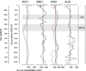
Figure 3.Drought atlas reconstructions over the Arctic for North America (NADA; Cook et al., 2004, https://www.ncdc.noaa.gov/paleo/ study/6319, last access: 16 January 2017) and Europe (OWDA; Cook et al., 2015, https://www.ncdc.noaa.gov/paleo/study/19419, last access: 4 November 2015). (a) The full spatial domains of the two atlases and a regional average over latitudes > 60◦N in (b) Europe and (c) North America transformed into z scores and filtered with a 100-year loess (red lines).
found in dark layers of well-humified peat, an indicator of dry conditions having allowed trees to grow and to colonise the area (Gunnarson, 2008).
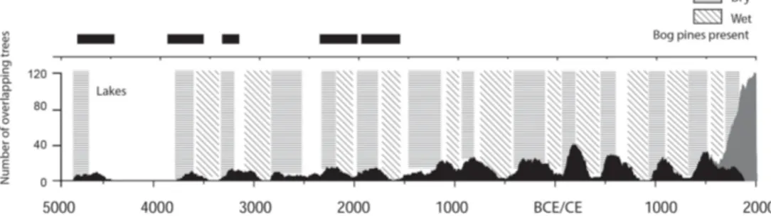
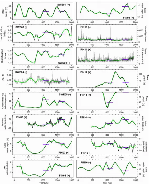
In west-central Sweden, more than 1000 subfossil and peatland Scots pine (Pinus sylvestris L.) samples have been collected since the late 1990s. Most samples come from dif-ferent lakes at varying altitudes, and the temporal distribu-tions of the dated samples show wave-like patterns of re-generation with clearly distinguishable mortality and ger-mination phases. Such generation pulses have been related to climatic conditions favourable for seed production and successful germination, i.e. warm and dry periods (Zack-risson et al., 1995). However, Gunnarson (2008) suggested that the temporal variations of pine samples from both bogs and lakes (Fig. 4) reflect fluctuations in peatland groundwa-ter tables and lake levels caused by regional changes in hy-droclimate. It is likely that these variations have been gov-erned by changes in precipitation rather than changes in
tem-perature. In south-eastern Finland evidence of depositional histories of subfossil pines from lakes, where most trees have grown adjacent to or on lakeshores (so-called ripar-ian trees), and peatland pines were combined by Helama et al. (2017a). Divergent depositional histories (i.e. replica-tion curves) were obtained for the two environments dur-ing the Common Era. High accumulation of peatland pines during the MCA indicates dry surface conditions beneficial for pine colonisation (Torbenson et al., 2015; Edvardsson et al., 2016). This phase overlapped with a phase of low ac-cumulation of riparian pine trees. In contrast, the accumula-tion of riparian pines increased towards the LIA, culminat-ing around 1300 CE and suggestculminat-ing a risculminat-ing lake water level contributing to tree mortality and increased preservation po-tential of trees in lakes. Again, this phase overlapped with a phase of strongly declined accumulation of peatland pine trees. These results were supported by taphonomic interpre-tation (Gastaldo, 1988) of the depositional histories,
espe-Figure 4.Changes in subfossil Scots pine (Pinus sylvestris L.) sample numbers over time (black) from lakes in the central Scandinavian Mountains (Gunnarson, 2008). The grey shaded area at the end represents living trees. Interpreted wet and dry periods shown in grey breaks and the presence of Scots pines growing on a nearby peat bog indicate drier conditions (figure adapted from Gunnarson, 2008). Data available at http://bolin.su.se/data/Gunnarson-2017 (last access: 22 June 2017).
cially their dissimilarities, and by comparisons with palae-olimnological reconstructions of water level fluctuations dur-ing the MCA and LIA (Luoto, 2009; Nevalainen et al., 2011; Nevalainen and Luoto, 2012). Similar to the study con-ducted in west-central Sweden (Gunnarson, 2008), the depo-sitional histories in south-eastern Finland were found to re-flect past hydroclimatic variations. Likely, the replication in pine chronologies from near the northern edge of the species range reflects summer temperature conditions, especially in subarctic sites (Helama et al., 2005, 2010). Further south, tree accumulation in different sediments seems to be more strongly influenced by recruitment and preservation poten-tials which, in turn are driven by local hydroclimatic condi-tions.
3.4 Glaciers
3.4.1 Glaciers as direct and indirect climate indicators Glaciers respond to climate changes through variations in length, area, and volume (Oerlemans, 1994, 2001). In the Arctic and subarctic, observations and indirect evidence of glacier fluctuations have been widely used as sources of in-formation about past climates (Solomina et al., 2016, and references therein). Changes in glacier length through ad-vances or retreats are indirect, lagged responses to climate change, while glacier mass balance variations, as indicated by changes in ice thickness and volume, are direct responses to the annual weather conditions (Haeberli and Hoelzle, 1995). Direct measurements of glacier variability across the world, derived from annual mass balance measurements us-ing glaciological or geodetic methods, are generally limited to the last half century (Zemp et al., 2009). In addition, annual mass balance records have been extended for sev-eral centuries using meteorological and proxy data such as historical records and tree-ring data (e.g. Lewis and Smith, 2004; Watson and Luckman, 2004; Nordli et al., 2005; Lin-derholm and Jansson, 2007). However, to yield information about glacier variability beyond direct observations, indirect indicators are mainly used.
There are two types of indirect glacier records: classi-cal discontinuous series usually based on moraines delim-iting the former glacier positions and continuous records from lakes (Solomina et al., 2016). Geomorphological ev-idence of glacier advances, such as terminal moraines or proglacial lacustrine sediments, give relative dates of glacier fluctuations, usually with some uncertainty. Lichenometry, a method through which lichen dimensions are used to in-fer the timing of colonisation, can provide rough estimates of moraine formation (Bickerton and Matthews, 1992; Arm-strong, 2004). If the moraines contain organic material, they can be dated by 14C (Karlén and Denton, 1976) or den-drochronological methods (Luckman, 1993; Carter et al., 1999). Cosmogenic isotopes (e.g.10Be) can be used to di-rectly identify the age of moraine deposition (Gosse and Phillips, 2001; Granger et al., 2013). Continuous records derived from lake sediment properties represent both the advance and retreat phases of glacier variations (Dahl and Nesje, 1994; Matthews et al., 2005; Bakke et al., 2008). As soon as the meltwater signal in proglacial lake sediments co-varies with the distance between the glacier and the lake, it can serve as an indicator of glacier extent and the corre-sponding equilibrium line altitude (ELA), which is the alti-tude where accumulation equals ablation (Dahl and Nesje, 1994). Reconstructions of the ELA are based on multi-proxy sediment analysis (e.g. loss on ignition, bulk density, mag-netic susceptibility grain-size distribution, and AMS dating control).
Glacier mass balance measurements demonstrate that for most regions summer temperature is the dominant control on annual mass balance (Koerner, 2005; Björnsson et al., 2013). Some exceptions have been noted; glacier advances in coastal areas of Scandinavia, SE Alaska, Kamchatka, and New Zealand in the late 20th century were forced primar-ily by high winter precipitation (e.g. Lemke et al., 2007). This means that in order to derive precipitation information from records of glacier variations, the data should be comple-mented by independent temperature reconstructions. Thus, if the advance of a glacier corresponds to inferred warm

![[PDF] Apprendre le jQuery | Cours PDF](data:image/gif;base64,R0lGODlhAQABAIAAAP///wAAACH5BAEAAAAALAAAAAABAAEAAAICRAEAOw==)