Towards real-time image understanding with convolutional networks

HAL Id: tel-01327221

https://pastel.archives-ouvertes.fr/tel-01327221

HAL is a multi-disciplinary open access

archive for the deposit and dissemination of sci-entific research documents, whether they are pub-lished or not. The documents may come from teaching and research institutions in France or

L’archive ouverte pluridisciplinaire HAL, est destinée au dépôt et à la diffusion de documents scientifiques de niveau recherche, publiés ou non, émanant des établissements d’enseignement et de recherche français ou étrangers, des laboratoires

Clement Farabet

To cite this version:

Clement Farabet. Towards real-time image understanding with convolutional networks. Computation and Language [cs.CL]. Université Paris-Est, 2013. English. �NNT : 2013PEST1083�. �tel-01327221�

A thesis submitted for the degree of

Docteur de l’universit´e Paris-Est en Informatique

Cl´

ement Farabet

Directeur de th`ese: Laurent Najman Co-Directeur de th`ese: Yann LeCun

Towards Real-Time

Image Understanding with

Convolutional Networks

December 19, 2013

Jury:

Yoshua Bengio (Pr´esident & Rapporteur)

L´eon Bottou (Rapporteur)

Eugenio Culurciello (Examinateur)

Sumit Chopra (Examinateur)

Laurent Najman (Directeur de th`ese)

One of the open questions of artificial computer vision is how to produce good internal representations of the visual world. What sort of internal representation would allow an artificial vision system to detect and classify objects into categories, independently of pose, scale, illumination, conforma-tion, and clutter? More interestingly, how could an artificial vision system learn appropriate internal representations automatically, the way animals and humans seem to learn by simply looking at the world?

Another related question is that of computational tractability, and more precisely that of computational efficiency. Given a good visual represen-tation, how efficiently can it be trained, and used to encode new sensorial data. Efficiency has several dimensions: power requirements, processing speed, and memory usage.

In this thesis I present three new contributions to the field of computer vision: (1) a multiscale deep convolutional network architecture to easily capture long-distance relationships between input variables in image data, (2) a tree-based algorithm to efficiently explore multiple segmentation can-didates, to produce maximally confident semantic segmentations of images, (3) a custom dataflow computer architecture optimized for the computation of convolutional networks, and similarly dense image processing models. All three contributions were produced with the common goal of getting us closer to real-time image understanding.

Scene parsing consists in labeling each pixel in an image with the category of the object it belongs to. In the first part of this thesis, I propose a method that uses a multiscale convolutional network trained from raw pixels to extract dense feature vectors that encode regions of multiple sizes centered on each pixel. The method alleviates the need for engineered features. In

covered by each node in the tree are aggregated and fed to a classifier which produces an estimate of the distribution of object categories contained in the segment. A subset of tree nodes that cover the image are then selected so as to maximize the average “purity” of the class distributions, hence maximizing the overall likelihood that each segment contains a single object. The system yields record accuracies on several public benchmarks.

The computation of convolutional networks, and related models heavily relies on a set of basic operators that are particularly fit for dedicated hardware implementations. In the second part of this thesis I introduce a scalable dataflow hardware architecture optimized for the computation of general-purpose vision algorithms—neuFlow —and a dataflow compiler— luaFlow —that transforms high-level flow-graph representations of these al-gorithms into machine code for neuFlow. This system was designed with the goal of providing real-time detection, categorization and localization of objects in complex scenes, while consuming 10 Watts when implemented on a Xilinx Virtex 6 FPGA platform, or about ten times less than a lap-top computer, and producing speedups of up to 100 times in real-world applications (results from 2011).

I would like to thank Prof. Yann LeCun for welcoming me into his intellec-tual circle, for sharing his long-term vision with me, and for continuously defining and redefining an exciting research field. While working on my PhD thesis, I enjoyed the freedom of exploration, while always benefiting from his full support and patience. It has been a great privilege and unique experience to grow as a researcher under his guidance.

I would like to thank Prof. Laurent Najman, my thesis adviser, for his continuous guidance during my thesis work. I’m infinitely grateful for his advice, patience and mentoring.

I would like to thank Eugenio Culurciello, Ronan Collobert, Camille Cou-prie, Marco Scoffier, Koray Kavukcuoglu, and Berin Martini for having been great collaborators, and all the people I have had fruitful discussions with, at Prof. Yann LeCun’s lab and outside.

I would also like to thank the members of my jury for their feedback on my thesis.

Finally, I am indebted to my wife, for her patience, and my parents, for putting me on the right tracks.

The research that led to this PhD thesis was conducted at the Courant Institute of Mathematical Sciences, New York University, over the course of 5 years, between 2008 and 2013. I officially registered as a PhD student at Universit´e Paris-Est from 2010 to 2013. This research was done in close collaboration with Prof. Yann LeCun at NYU, and with Prof. Laurent Najman at Universit´e Paris-Est. The work on neuFlow (Chapter 3) started as a Master’s thesis/project in 2008.

Journals

C. Farabet, C. Couprie, L. Najman and Y. LeCun, “Learning Hierar-chical Features for Scene Labeling”, IEEE Transactions on Pattern Analysis and Machine Intelligence, in press, 2013.

C. Farabet, R. Paz, J. Perez-Carrasco, C. Zamarreno, A. Linares-Barranco, Y. LeCun, E. Culurciello, T. Serrano-Gotarredona and B. Linares-Barranco, “Comparison Between Frame-Constrained Fix-Pixel-Value and Frame-Free Spiking-Dynamic-Pixel ConvNets for Visual Process-ing”, in Frontiers in Neuroscience, 2012.

C. Farabet, Y. LeCun, K. Kavukcuoglu, B. Martini, P. Akselrod, S. Talay, and E. Culurciello, “Large-Scale FPGA-Based Convolutional Networks”, in R. Bekkerman, M. Bilenko, and J. Langford (Ed.), Scaling Up Machine Learning, Cambridge University Press, 2011.

International Conferences

C. Couprie, C. Farabet, L. Najman, Y. LeCun, “Indoor Semantic Segmentation using depth information”, in Proceedings of the International Conference on Learning Representations, May 2013.

C. Culurciello, J. Bates, A. Dundar, J. Carrasco, C. Farabet, “Clustering Learning for Robotic Vision”, ArXiv preprint, January 2013, in Proceedings of the International Conference on Learning Representations, May 2013.

C. Farabet, C. Couprie, L. Najman, Y. LeCun, “Scene Parsing with Multiscale Feature Learning, Purity Trees, and Optimal Covers”, in Proc. of

Phi-Hung Pham, Darko Jelaca, Clement Farabet, Berin Martini, Yann LeCun and Eugenio Culurciello, “NeuFlow: Dataflow Vision Processing System-on-a-Chip”, in IEEE International Midwest Symposium on Circuits and systems, IEEE MWSCAS, 2012, Boise, Idaho, USA. C. Farabet, B. Martini, B. Corda, P. Akselrod, E. Culurciello and Y. LeCun, “NeuFlow: A Runtime Reconfigurable Dataflow Processor for Vision”, in Proc. of the Fifth IEEE Workshop on Embedded Computer Vi-sion (ECV’11 @ CVPR’11), IEEE, Colorado Springs, 2011. Invited Paper. C. Farabet, B. Martini, P. Akselrod, S. Talay, Y. LeCun and E. Culurciello, “Hardware Accelerated Convolutional Neural Networks for Synthetic Vision Systems”, in International Symposium on Circuits and Systems (ISCAS’10), IEEE, Paris, 2010.

Y. LeCun, K. Kavukcuoglu and C. Farabet, “Convolutional Networks and Applications in Vision”, in International Symposium on Circuits and Systems (ISCAS’10), IEEE, Paris, 2010.

C. Farabet, C. Poulet and Y. LeCun, “An FPGA-Based Stream Pro-cessor for Embedded Real-Time Vision with Convolutional Networks”, in Proc. of the Fifth IEEE Workshop on Embedded Computer Vision (ECV’09 @ ICCV’09), IEEE, Kyoto, 2009.

C. Farabet, C. Poulet, J. Y. Han and Y. LeCun, “CNP: An FPGA-based Processor for Convolutional Networks”, in International Conference on Field Programmable Logic and Applications (FPL’09), IEEE, Prague, 2009.

Software, Patent

R. Collobert, K. Kavukcuoglu, C. Farabet, “Torch7: A Matlab-like Environment for Machines Learning”, in Big Learning Workshop (@ NIPS’11), Sierra Nevada, Spain, 2011. http://www.torch.ch

List of Figures xi

List of Tables xiii

1 Introduction 1

1.1 Representation Learning with Deep Networks . . . 3

1.1.1 Deep Network Architectures . . . 3

1.1.1.1 Multilayer Perceptrons . . . 4

1.1.1.2 Convolutional Networks . . . 5

1.1.1.3 Encoders + Decoders = Auto-encoders . . . 9

1.1.2 Learning: Parameter Estimation . . . 11

1.1.2.1 Loss Function, Objective . . . 11

1.1.2.2 Optimization . . . 12

1.2 Hierarchical Segmentations, Structured Prediction . . . 12

1.2.1 Hierarchical Segmentations . . . 13

1.2.1.1 Graph Representation . . . 13

1.2.1.2 Minimum Spanning Trees . . . 15

1.2.1.3 Dendograms . . . 16

1.2.1.4 Segmentations . . . 16

1.2.2 Structured Prediction . . . 17

1.2.2.1 Graphical Models . . . 18

1.2.2.2 Learning: Parameter Estimation . . . 19

2 Image Understanding: Scene Parsing 25

2.1 Introduction . . . 25

2.2 A Model for Scene Understanding . . . 25

2.2.1 Introduction . . . 25

2.2.2 Multiscale feature extraction for scene parsing . . . 29

2.2.2.1 Scale-invariant, scene-level feature extraction . . . 30

2.2.2.2 Learning discriminative scale-invariant features . . . 32

2.2.3 Scene labeling strategies . . . 33

2.2.3.1 Superpixels . . . 33

2.2.3.2 Conditional Random Fields . . . 34

2.2.3.3 Parameter-free multilevel parsing . . . 36

2.2.4 Experiments . . . 41

2.2.4.1 Multiscale feature extraction . . . 44

2.2.4.2 Parsing with superpixels . . . 45

2.2.4.3 Multilevel parsing . . . 46

2.2.4.4 Conditional random field . . . 47

2.2.4.5 Some comments on the learned features . . . 47

2.2.4.6 Some comments on real-world generalization . . . 47

2.2.5 Discussion and Conclusions . . . 48

3 A Hardware Platform for Real-time Image Understanding 57 3.1 Introduction . . . 57

3.2 Learning Internal Representations . . . 58

3.2.1 Convolutional Networks . . . 59

3.2.2 Unsupervised Learning of ConvNets . . . 62

3.2.2.1 Unsupervised Training with Predictive Sparse Decom-position . . . 62

3.2.2.2 Results on Object Recognition . . . 63

3.2.2.3 Connection with Other Approaches in Object Recognition 64 3.3 A Dedicated Digital Hardware Architecture . . . 65

3.3.1 A Data-Flow Approach . . . 66

3.3.1.1 On Runtime Reconfiguration . . . 68

3.3.2.1 Specialized Processing Tiles . . . 74

3.3.2.2 Smart DMA Implementation . . . 75

3.3.3 Compiling ConvNets for the ConvNet Processor . . . 76

3.3.4 Application to Scene Understanding . . . 78

3.3.5 Performance . . . 81

3.3.6 Precision . . . 84

4 Discussion 87

1.1 Common ConvNet Blocks . . . 7

1.2 Graphs with local connectivity . . . 14

1.3 Gradient graph . . . 14

1.4 Minimum Spanning Tree of a Graph . . . 15

1.5 Dendogram of an MST . . . 16

1.6 Cutting the Dendogram = Segmenting . . . 17

1.7 Von Neumann Architecture . . . 22

1.8 Our Proposed Dataflow Architecture . . . 24

2.1 Model overview . . . 27

2.2 Superpixels . . . 34

2.3 CRFs . . . 35

2.4 Optimal Cover . . . 37

2.5 Optimal Cover on a Tree: . . . 39

2.6 Max Sampling . . . 40

2.7 Scene Parsing Results . . . 52

2.8 More Scene Parsing Results . . . 53

2.9 Scene Parsing Results with More Classes . . . 53

2.10 Learned Filters . . . 54

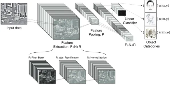
3.1 Architecture of a typical convolutional network for object recognition. This implements a convolutional feature extractor and a linear classifier for generic N-class object recognition. Once trained, the network can be computed on arbitrary large input images, producing a classification map as output. . . 59 3.2 A data-flow computer. A set of runtime configurable processing tiles are

connected on a 2D grid. They can exchange data with their 4 neighbors and with an off-chip memory via global lines. . . 67 3.3 The grid is configured for a complex computation that involves several

tiles: the 3 top tiles perform a 3 × 3 convolution, the 3 intermediate tiles another 3 × 3 convolution, the bottom left tile sums these two convolu-tions, and the bottom centre tile applies a function to the result. . . 71 3.4 Overview of the ConvNet Processor system. A grid of multiple

full-custom Processing Tiles tailored to ConvNet operations, and a fast streaming memory interface (Smart DMA). . . 73 3.5 Scene Parsing on FPGAs . . . 79 3.6 Compute time for a typical ConvNet (as seen in Figure 3.1). . . 82 3.7 Quantization effect on trained networks: the x axis shows the fixed point

position, the y axis the percentage of weights being zeroed after quanti-zation. . . 86

2.1 Performance of our system on the Stanford Background dataset . . . 42 2.2 Performance of our system on the SIFT Flow dataset . . . 42 2.3 Performance of our system on the Barcelona dataset . . . 44 3.1 Average recognition rates on Caltech-101 with 30 training samples per

class. Each row contains results for one of the training protocols (U = unsupervised, X = random, + = supervised fine-tuning), and each column for one type of architecture (F = filter bank, PA = average pooling, PM = max pooling, R = rectification, N = normalization). . . 63 3.2 CN1: base model. N: Local Normalization layer (note: only the Y

channel is normalized, U and V are untouched); C: convolutional layer; P: pooling (max) layer; L: linear classifier. . . 81 3.3 CN2: second model. Filters are increased, which doubles the receptive

field . . . 83 3.4 CN3: a fourth convolutional layer C6 is added, which, again, increases

the receptive field. Note: C6 has sparse connectivity (e.g.each of its 128 outputs is connected to 8 inputs only, yielding 1024 kernels instead of 6144). . . 84 3.5 Percentage of mislabeled pixels on validation set. CN Error is the

pixel-wise error obtained when using the simplest pixelpixel-wise winner, predicted by the ConvNet. CN+MST Error is the pixelwise error obtained by his-togramming the ConvNet’s prediction into connected components (the components are obtained by computing the minimum spanning tree of an edge-weighted graph built on the raw RGB image, and merging its nodes using a surface criterion, in the spirit of (35)). . . 84

3.6 Performance comparison. 1- CPU: Intel DuoCore, 2.7GHz, optimized C code, 2- V6: neuFlow on Xilinx Virtex 6 FPGA—on board power and GOPs measurements; 3- IBM: neuFlow on IBM 45nm process: simulated results, the design was fully placed and routed; 4- mGPU/GPU: two GPU implementations, a low power GT335m and a high-end GTX480. . 85

Introduction

Central to this thesis is the question: how can we enable computers to automatically and efficiently understand images? Understand being an ambiguous term, we start with a few definitions. From the dictionary:

Definition 1 — understand:

(1) to perceive the meaning of; grasp the idea of; comprehend. (2) to assign a meaning to; interpret.

(3) to have a systematic interpretation or rationale, as in a field or area of knowledge. Definition 2 — image:

an optical counterpart or appearance of an object, as is produced by reflection from a mirror, refraction by a lens, or the passage of luminous rays through a small aperture and their reception on a surface.

From these we can provide our own definition: Definition 3 — understand an image:

(1) to perceive the meaning behind the formation of the image

(2) to systematically interpret the causes—the physical objects and events—that resulted in the formation of the image.

This definition is not perfect, but it gives us a scope for this thesis. From this, it is easy to see how vast the task of understanding an image can be. Given the pixels, one would have to infer all the causes that led to this image: lighting conditions, exact list of all objects present in the receptive field, their exact 3D positions, contours, colors, surface normals. . .

In this thesis I focus on a subset of these explaining factors, which is commonly referred to as semantic labeling, or image parsing:

Definition 4 — parse an image:

given an image (an array of pixels), produce a 2D map (in the plane of the image) of objects, with their precise contour, position, and label (from a pre-defined label set).

The task of image parsing is significantly simpler than the task of full image under-standing, and yet captures most of its fundamental problems: representation, recogni-tion, segmentation. . .

The core of my thesis can be broken up into three main contributions:

1. a multiscale deep convolutional network architecture to easily capture long-distance relationships between input variables in image data. This type of model produces invariant yet spatially accurate features, which provide a good basis for image parsing,

2. a tree-based algorithm to efficiently explore multiple segmentation candidates, to produce maximally confident semantic segmentations of images. This type of method is computationally efficient, and provides a simple-to-use post-processing framework for image parsing,

3. a custom dataflow computer architecture optimized for the computation of con-volutional networks, and similarly dense image processing models. This computer is fully implemented and functional.

The goal of this introduction is to put each contribution in perspective, and better understand where they come from, with one section per contribution. I start with a review of representation learning using deep networks. The second section provides context on the problem of structured prediction, and the use of segmentation trees. The third section describes dataflow computers, and why they are particularly well suited compute models for data-intensive tasks such as image parsing.

1.1

Representation Learning with Deep Networks

“Deep learning is just a buzzword for neural nets, and neural nets are just a stack of matrix-vector multiplications, interleaved with some

non-linearities. No magic there.”

— Ronan Collobert, 2011 (24)

One of the key questions of Vision Science (natural and artificial) is how to produce good internal representations of the visual world. What sort of internal representation would allow an artificial vision system to detect and classify objects into categories, independently of pose, scale, illumination, conformation, and clutter? More interest-ingly, how could an artificial vision system learn appropriate internal representations automatically, the way animals and humans seem to learn by simply looking at the world? In the time-honored approach to computer vision (and to pattern recognition in general), the question is avoided: internal representations are produced by a hand-crafted feature extractor, whose output is fed to a trainable classifier. While the issue of learning features has been a topic of interest for many years, considerable progress has been achieved in the last few years with the development of so-called deep learning methods.

Good internal representations are hierarchical. In vision, pixels are assembled into edglets, edglets into motifs, motifs into parts, parts into objects, and objects into scenes. This suggests that recognition architectures for vision (and for other modalities such as audio and natural language) should have multiple trainable stages stacked on top of each other, one for each level in the feature hierarchy. Deep neural networks are particularly well suited to represent hierarchical signals, as the overall function is naturally decomposed into a hierarchy of simpler, linear functions. Convolutional neural networks are an extension of deep neural networks, in which each layer imposes spatial (or temporal) replication of the weights, to exploit the stationarity and locality of the signal at each layer.

1.1.1 Deep Network Architectures

1.1.1.1 Multilayer Perceptrons

The first deep network, or deep learner, was the multilayer perceptron (MLP). An MLP typically consists of multiple layers of nodes arranged in a directed graph, with each layer fully connected to the next one. A node, or neuron at each layer is produced by a non-linear activation function of a linear combination of activations at the previous layer.

Mathematically, an MLP with L layers can be described by these simple equations:

y = f (x; θ) = hL, (1.1)

hl= actl(Wlhl−1+ bl) ∀ l ∈ {1, . . . , L − 1}, (1.2)

h0 = x, (1.3)

with bla vector of trainable bias parameters, Wla matrix of trainable weights, x is the input vector, y is a vector of output units, θ is a vector that represents all the trainable parameters {Wl, bl} ∀ l ∈ {1, . . . , L}, and actl is a non-linear activation function at layer l.

The most commonly used activation function for the hidden units actl ∀ l ∈ {1, . . . , L − 1}) is tanh, but other more exotic transfer functions, such as the rectified linear unit (ReLU) can be used to effectively train deeper architectures. The output activation function actL depends on the problem at hand. For regression problems, it can be a simple linear function, or a log-linear function. For discrimination problems, the softmax function is the most widely used, for its connection to maximum a poste-riori probability (MAP) estimation. The softmax normalizes the output units so that they sum to 1, which turns the MLP into an approximator for the posterior probability P (Y = tn_|xn_{, θ). When using a softmax activation function, the training procedure} becomes analogous to MAP estimation in the sense that we seek the training parameter vector θ that maximizes the likelihood over all training samples {xn, tn}.

Note: some textbooks consider the input vector x as a layer. In this thesis I only count the hidden layers and the output layer. This way, a simple linear model is considered a one-layer model, whereas the smallest MLP is considered a two-layer model (with one hidden layer). Effectively, I’m counting each linear projection as a layer.

1.1.1.2 Convolutional Networks

Many successful object recognition systems use dense features extracted on regularly-spaced patches over the input image. The majority of the feature extraction systems have a common structure composed of a filter bank (generally based on oriented edge detectors or 2D gabor functions), a non-linear operation (quantization, winner-take-all, sparsification, normalization, and/or point-wise saturation) and finally a pooling oper-ation (max, average or histogramming). For example, the scale-invariant feature trans-form (SIFT (73)) operator applies oriented edge filters to a small patch and determines the dominant orientation through a winner-take-all operation. Finally, the resulting sparse vectors are added (pooled) over a larger patch to form local orientation his-tograms. Some recognition systems use a single stage of feature extractors (28, 60, 87). Other models like HMAX-type models (77, 93) and convolutional networks use two or more layers of successive feature extractors.

Put simply, Convolutional Networks (64, 65), or ConvNets are an extension of mul-tilayer perceptrons, where the basic linear layers are replaced by convolutional layers. Non-linear activations are commonly followed by a spatial pooling function, which en-forces low-level shift invariance.

Mathematically, a ConvNet with L layers can be described as an MLP, where we write the states as matrices (or more precisely arrays, or collections of vectors):

Y = f (X; θ) = HL, (1.4)

Hl= pooll(actl(WlHl−1+ bl)) ∀ l ∈ {1, . . . , L − 1}, (1.5)

H0 = X, (1.6)

with bl a vector of trainable bias parameters, Wl a matrix of trainable weights, X is the input array of vectors (an image is an array of pixels), Y is an array of output vectors (each vector encodes a sub-window of the input), θ is a vector that represents all the trainable parameters {Wl, bl} ∀ l ∈ {1, . . . , L}, actl is a non-linear activation function at layer l, and pool_l is a pooling function at layer l.

The major difference with the MLP is that the matrices Wl are Toeplitz matrices, therefore each hidden unit array Hl can be expressed as a regular convolution between kernels from Wl and the previous hidden unit vector Hl−1, squashed through an actl

function, and pooled spatially. More specifically, Hlp = pool(act(blp+

X q∈parents(p)

wlpq∗ Hl−1,q)). (1.7)

The hidden units Hl are commonly called feature vector maps, and Hlp is called a feature map. Concretely, if the input is a color image, each feature map would be a 2D array containing a color channel of the input image (for an audio input each feature map would be a 1D array, and for a video or volumetric image, it would be a 3D array). At the output, each feature map represents a particular feature extracted at all locations on the input.

From the mathematical description above, we can identify three key building blocks of ConvNets: the convolutional layer, or filter bank layer, the activation function, or non-linearity layer, and the pooling function, or feature pooling layer. A typical Conv-Net is composed of one, two or more such 3-layer stages. The output of a ConvConv-Net is usually fed into an simple linear classifier, or, more generally into an MLP. From the training/optimization point of view, the complete stack (ConvNet+MLP) can be treated as an MLP: for discriminative tasks, the usual softmax activation function is used as the output activation module, so that the optimization becomes a MAP esti-mation problem.

We now describe these three building blocks, which are used extensively throughout this thesis (see Figure 1.1):

Filter Bank Layer - F : the input is a 3D array with n1 2D feature maps of size n2× n3. Each component is denoted xijk, and each feature map is denoted xi. The output is also a 3D array, y composed of m1 feature maps of size m2× m3. A trainable filter (kernel) kij in the filter bank has size l1× l2 and connects input feature map xi to output feature map yj. The module computes yj = bj+Pikij∗ xi where ∗ is the 2D discrete convolution operator and bj is a trainable bias parameter. Each filter detects a particular feature at every location on the input. Hence spatially translating the input of a feature detection layer will translate the output but leave it otherwise unchanged. Non-Linearity Layer: In traditional ConvNets this simply consists in a pointwise tanh() sigmoid function applied to each site (ijk). However, recent implementations have used more sophisticated non-linearities. A useful one for natural image recognition is the rectified sigmoid Rabs: abs(gi.tanh()) where gi is a trainable gain parameter. The

■ ✁ ✂ ✄☎ ✆ ✄✆ ❋ ✝✆ ✄✂✞ ✝ P ✟ ✟✠ ✡ ☛ ☞P ▲ ✡ ✝✆✞ ❈✠✆✌ ✌✡✍✡✝ ✞ ❋ ✝✆ ✄✂✞ ✝ ❊✎ ✄✞✆ ✏ ✄✡✟ ☞❋✑✒✑✓ ❋✑✒✑✓ ④ ✔✕✖✗✘ ✐✱✙ ✐✮ ❖ ✚ ✛✝✏ ✄ ❈✆ ✄✝☛ ✟✞✡✝✌ ④ ✔✕✖✗✘ ❥✱✙ ❥✮ ④ ✔✕ ✖✗✘❦✱✙❦✮ ❘✜✢✣✤ ✥❘✦✧ ★✩✪ ✩✧ ✢★✩ ✫✬ ✭✥✭✩✯★✦✰❇✢✬✲ ◆ ✥◆ ✫✰✳ ✢✯✩❧ ✢ ★✩✫✬

Figure 1.1: Common ConvNet Blocks - Architecture of a typical convolutional network for object recognition. This implements a convolutional feature extractor and a linear classifier for generic N-class object recognition. Once trained, the network can be computed on arbitrary large input images, producing a classification map as output.

rectified sigmoid is sometimes followed by a subtractive and divisive local normalization N , which enforces local competition between adjacent features in a feature map, and be-tween features at the same spatial location. The subtractive normalization operation for a given site xijk computes: vijk= xijk−P_ipqwpq.xi,j+p,k+q, where wpq is a normalized truncated Gaussian weighting window (typically of size 9x9). The divisive normaliza-tion computes yijk = vijk/max(mean(σjk), σjk) where σjk = (Pipqwpq.vi,j+p,k+q2 )1/2. The local contrast normalization layer is inspired by visual neuroscience models (74, 87). Feature Pooling Layer: This layer treats each feature map separately. In its simplest instance, called PA, it computes the average values over a neighborhood in each feature map. The neighborhoods are stepped by a stride larger than 1 (but smaller than or equal to the pooling neighborhood). This results in a reduced-resolution output feature map which is robust to small variations in the location of features in the previous layer. The average operation is sometimes replaced by a max PM. Traditional ConvNets use a pointwise tanh() after the pooling layer, but more recent models do not. Some ConvNets dispense with the separate pooling layer entirely, but use strides larger than one in the filter bank layer to reduce the resolution (63, 96). In some recent

versions of ConvNets, the pooling also pools different features at a same location, in addition to the same feature at nearby locations (54).

(A Short History of ConvNets)

ConvNets can be seen as a representatives of a wide class of models that we will call Multi-Stage Hubel-Wiesel Architectures. The idea is rooted in Hubel and Wiesel’s classic 1962 work on the cat’s primary visual cortex. It identified orientation-selective simple cells with local receptive fields, whose role is similar to the ConvNets filter bank layers, and complex cells, whose role is similar to the pooling layers. The first such model to be simulated on a computer was Fukushima’s Neocognitron (38), which used a layer-wise, unsupervised competitive learning algorithm for the filter banks, and a separately-trained supervised linear classifier for the output layer. The innovation in (63, 64) was to simplify the architecture and to use the back-propagation algorithm to train the entire system in a supervised fashion. The approach was very successful for such tasks as OCR and handwriting recognition. An operational bank check reading system built around ConvNets was developed at AT&T in the early 1990’s (65). It was first deployed commercially in 1993, running on a DSP board in check-reading ATM machines in Europe and the US, and was deployed in large bank check reading machines in 1996. By the late 90’s it was reading over 10% of all the checks in the US. This motivated Microsoft to deploy ConvNets in a number of OCR and handwriting recognition systems (18, 19, 96) including for Arabic (1) and Chinese characters (17). Supervised ConvNets have also been used for object detection in images, including faces with record accuracy and real-time performance (40, 80, 84, 101), Google recently deployed a ConvNet to detect faces and license plate in StreetView images so as to protect privacy (37). NEC has deployed ConvNet-based system in Japan for tracking customers in supermarket and recognizing their gender and age. Vidient Technologies has developed a ConvNet-based video surveillance system deployed in several airports in the US. France T´el´ecom has deployed ConvNet-based face detection systems for video-conference and other systems (40). Other experimental detection applications include hands/gesture (82), logos and text (29). A big advantage of ConvNets for detection is their computational efficiency: even though the system is trained on small windows, it suffices to extend the convolutions to the size of the input image and replicate the output layer to compute detections at every location. Supervised ConvNets have also been used for vision-based obstacle avoidance for off-road mobile robots (67). Two participants

in the recent DARPA-sponsored LAGR program on vision-based navigation for off-road robots used ConvNets for long-range obstacle detection (45, 46). In (45), the system is pre-trained off-line using a combination of unsupervised learning (as described in section 3.2.2) and supervised learning. It is then adapted on-line, as the robot runs, using labels provided by a short-range stereovision system (see videos at http:// www.cs.nyu.edu/~yann/research/lagr). Interesting new applications include image restoration (50) and image segmentation, particularly for biological images (81). The big advantage over graphical models is the ability to take a large context window into account. Stunning results were obtained at MIT for reconstructing neuronal circuits from a stack of brain slice images a few nanometer thick (51).

Over the years, other instances of the Multi-Stage Hubel-Wiesel Architecture have appeared that are in the tradition of the Neocognitron: unlike supervised ConvNets, they use a combination of hand-crafting, and simple unsupervised methods to design the filter banks. Notable examples include Mozer’s visual models (75), and the so-called HMAX family of models from T. Poggio’s lab at MIT (77, 93), which uses hard-wired Gabor filters in the first stage, and a simple unsupervised random template selection algorithm for the second stage. All stages use point-wise non-linearities and max pooling. From the same institute, Pinto et al. (87) have identified the most appropriate non-linearities and normalizations by running systematic experiments with a single-stage architecture using GPU-based parallel hardware.

1.1.1.3 Encoders + Decoders = Auto-encoders

Training deep, multi-stage architectures using supervised gradient back propagation requires many labeled samples. However in many problems labeled data is scarce whereas unlabeled data is abundant. Recent research in deep learning (7, 48, 88) has shown that unsupervised learning can be used to train each stage one after the other using only unlabeled data, reducing the requirement for labeled samples significantly.

Learning features in an unsupervised manner (i.e. without labels) can be achieved simply, by using auto-encoders. An auto-encoder is a model that takes a vector input y, maps it into a hidden representation z (code) using an encoder which typically has the form:

where act is a non-linear activation function, We the encoding matrix and bea vector of bias parameters.

The hidden representation z, often called code, is then mapped back into the space of y, using a decoder of this form:

˜

y = Wdz + bz, (1.9)

where Wd is the decoding matrix and bd a vector of bias parameters.

The goal of the auto-encoder is to minimize the reconstruction error, which is rep-resented by a distance between y and ˜y. The most common type of distance is the mean squared error ||y − ˜y||2₂.

The code z typically has less dimensions than y, which forces the auto-encoder to learn a good representation of the data. In its simplest form (linear), an auto-encoder learns to project the data onto its first principal components. If the code z has as many components as y, then no compression is required, and the model could typically end up learning the identity function. Now if the encoder has a non-linear form (using a tanh, or using a multi-layered model), then the auto-encoder can learn a potentially more powerful representation of the data.

Basic auto-encoders require a number of tricks and know how to properly train them, and avoid the pitfall of learning the identity function. In practice, using a code y that is smaller than x is enough to avoid learning the identity, but it remains hard to do much better than PCA. Techniques like the denoising auto-encoder (DAE), introduced in (102) can be useful to avoid that.

Using codes that are over-complete (i.e. with more components than the input) makes the problem even worse. There are different ways that an auto-encoder with an over-complete code may still discover interesting representations. One common way is the addition of sparsity: by forcing units of the hidden representation to be mostly 0s, the auto-encoder has to learn a distributed representation of the data. More advanced methods, such as Predictive Sparse Coding (PSD) (53), involve learning an encoder that approximates the exact result of sparse coding. Sparse Coding can be a bit costly, as it is an iterative procedure, whereas the encoder will predict the sparse code in a feedforward way.

The auto-encoder loss can be used by itself for purely unsupervised pre-training. The parameters are then used to initialize the supervised procedure. It can also be

used in conjunction with the supervised training, to ensure that there is no loss of information at each layer: if the auto-encoder loss is perfectly minimized, it means that the top layer representation contains all the information required to rebuild the input signal. This can be useful for tasks where certain labels have too few training examples, such that it is dangerous to rely on the label information alone.

1.1.2 Learning: Parameter Estimation

In this thesis I focus on deep networks for discriminative tasks. Therefore, I will only consider learning (parameter estimation) for discriminative tasks.

1.1.2.1 Loss Function, Objective

From the point of view of parameter estimation, the architecture of the model can usually be abstracted. In the following, we assume a training set of N training samples {xn, tn}, with xn an input example, and tn a target value, or label, associated to that example; tn_{∈ {1, . . . , K}, with K the number of possible target classes. We can write:} yn= f (xn; θ) ∀ n ∈ {1, . . . , N }, (1.10) l(f ; xn, tn, θ) = l(f (xn; θ), tn) ∀ n ∈ {1, . . . , N } (1.11)

L(f ; x, t, θ) = X n∈{1,...,N }

l(f ; xn, tn, θ) (1.12)

where f is a model with trainable parameters θ, l is a loss function which captures the per-sample objective to be optimized, and L the global loss function which represents the overall objective to be optimized.

As described in Section 1.1.1, the use of a softmax output activation function allows us to turn the learning problem into a likelihood maximization problem, or negative log-likelihood minimization problem, which gives:

l(f (xn; θ), tn) = − log(P (Y = tn|xn, θ)) (1.13)

= − log(f (xn)). (1.14)

There are several other types of possible loss functions, but the negative log-likelihood (NLL) provides a simple and consistent parameter estimation framework, in which the outputs of f are properly calibrated units.

1.1.2.2 Optimization

Once a model f and a loss function l have been chosen, we can define the task of learning, or parameter estimation, as minimizing the loss function L over the training set {xn_{, t}n_{} ∀ n ∈ {1, . . . , N }. If f and l are differentiable, or at least piece-wise} differentiable, this optimization can be cast as a gradient descent procedure.

The most naive way to go about solving this optimization problem is to compute the derivative of the loss function with respect to all the trainable parameters (using the well-known backpropagation algorithm), over the complete training set, and then follow the opposite direction to update the parameters. It is naive for two reasons: (1) it only relies on first order information (the gradient), (2) it relies on the entire dataset to evaluate the gradient (full batch), which is typically extremely inefficient.

The first point can be addressed using parameter normalization, hidden unit nor-malization, (partial) second-order information. . . Different types of normalizations are presented throughout this thesis.

The second point is typically addressed using a stochastic approximation of the gradient, usually referred to as stochastic gradient descent (SGD). The most extreme form of SGD is when a single sample {xn_{, t}n_{} is used to estimate the gradient, and} to update the parameters. We usually use the term mini-batch to describe the set of samples used to evaluate the gradient and update the parameters. The mini-batch size can vary from 1 (pure SGD) to N (batch method, or exact method).

All the algorithms presented in this thesis rely on some form of stochasticity. Several studies (11, 12, 13) have shown that even when f is a convex function with respect to the trainable parameters, SGD yields significantly faster convergence, and when combined to a proper learning rate schedule and/or validation scheme, reaches the same accuracy as exact methods. SGD was used extensively in this thesis.

1.2

Hierarchical Segmentations, Structured Prediction

The focus of this thesis is on image understanding, and more precisely on image parsing, or multi-label segmentation. Although it is theoretically doable to build a deep model f which can remap a raw image signal X into a map of discrete labels, the use of heuristics—candidate segmentations—can greatly speedup the learning process, and the overall consistency of image labelings.

In this section I provide material and context for Chapter 2. I start with an intro-duction on hierarchical segmentations, which are used throughout Chapter 2. I then present the general ideas of structured prediction, a good paradigm for sequence data and spatial data labeling problems.

1.2.1 Hierarchical Segmentations

An image segmentation is a partitioning of an image into regions corresponding to different objects. A hierarchical image segmentation is an ensemble of image segmen-tations where the image segments are arranged in a tree-like structure. The root of the tree is a single segment that spans all the pixels of the image, and the leaves of the tree are the individual pixels (one component per pixel). This type of data structure is particularly useful to explore different levels of candidate segmentations.

In this section, I describe the basics required to build graphs on images, and produce hierarchical segmentations on these graphs.

1.2.1.1 Graph Representation

A graph G is defined by a set of vertices V and a set of edges E that connect the vertices. In this thesis, we use the convention of edge-weighted, undirected graphs, to represent images: a pixel is represented by a vertex, and a link between two pixels is represented by a weighted edge.

A complete graph over an image is defined when each pixel is connected to every other pixel in the image. Such graph is typically very costly to represent in memory, as its number of edges scales quadratically with the number of pixels.

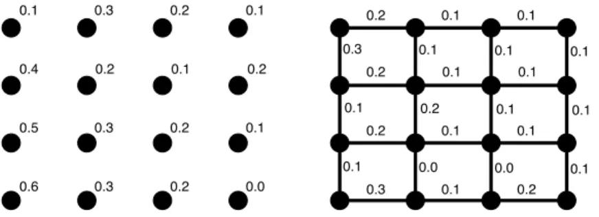
A much more common type of graph is locally connected: each pixel is connected to its most immediate 4 neighbors (4-connexity) or its 8 immediate neighbors (8-connexity), as shown on Figure 1.2.

A very simple and natural kind of graph is a gradient graph: such a graph can be built by setting the connexity to 4, and assigning each edge a weight that is the Eu-clidean distance between its two neighboring vertices. This graph represents a gradient map: each edge encodes a distance between pixels, as shown on Figure 1.3.

Figure 1.2: Graphs with local connectivity - Left: 4-connexity. Right: 8-connexity. 0.1 0.3 0.2 0.1 0.2 0.1 0.2 0.4 0.5 0.3 0.2 0.1 0.6 0.3 0.2 0.0 0.2 0.1 0.1 0.1 0.1 0.1 0.1 0.2 0.2 0.1 0.1 0.1 0.3 0.1 0.2 0.1 0.1 0.0 0.1 0.2 0.0 0.3 0.1 0.1

Figure 1.3: Gradient graph - This type of graph is edge-weighted. Left: vertices, with weights attached. Right: the edge-weighted gradient graph—each edge has a weight associated, which is produced by the distance between its two neighboring vertices.

1.2.1.2 Minimum Spanning Trees

Once a graph is constructed over an image, we can start thinking about trees. A spanning tree of a graph G is itself a graph T , that contains all the vertices of G but a subset of the edges in G that span all the vertices. For a given graph G over an image, there are multiple possible spanning trees. A minimum spanning tree TM ST of an edge-weighted graph G is the subset of edges chosen such that they minimize the sum of the edge weights. A key property of spanning trees is that they contain no loops (which is why they are called trees!).

0.2 0.1 0.1 0.1 0.1 0.1 0.1 0.2 0.2 0.1 0.1 0.1 0.3 0.1 0.2 0.1 0.1 0.0 0.1 0.2 0.0 0.3 0.1 0.1 0.2 0.1 0.1 0.1 0.1 0.1 0.1 0.2 0.1 0.1 0.1 0.0 0.0 0.1 0.1

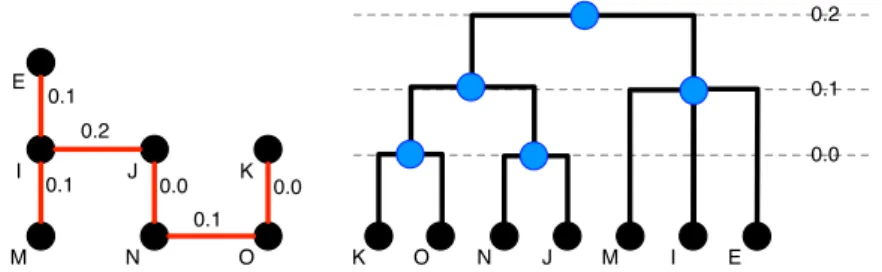
Figure 1.4: Minimum Spanning Tree of a Graph - Left: highlighting a possible MST for the graph in Figure 1.2. Right: pruning the graph to only keep the edges belonging to the MST—these edges cover the graph.

There are multiple well-known algorithms for finding MSTs. One of them is Kruskal’s algorithm (56, 79), which constructs the MST by sorting all the edges by increasing weight, and adds them one by one if they do not create cycles. The algorithm main-tains a list of clusters, and ensures that each time it adds an edge to the MST, the edge fuses two distinct clusters (if the two neighboring vertices already belonged to the same cluster, then adding that extra edge would create a cycle). Thus the only challenge of the Kruskal algorithm is to efficiently keep track of the clusters. Using disjoint sets and path compression, the overall complexity of the algorithm can be kept to O(|E|.α(|E|)), where |E| is the number of edges in the graph, and α(.) is the inverse Ackermann function, a function that grows very slowly with its argument. In other terms, the Kruskal algorithm is roughly linear in the number of edges, when correctly implemented.

This is an important conclusion, as it tells us that we can compute minimum span-ning trees very cheaply.

1.2.1.3 Dendograms

A minimum spanning tree is an efficient data structure to access a grid of pixels, and have them organized by increasing edge weights. But the minimum spanning tree is in fact more informative: it actually captures a full segmentation hierarchy. To see that, the spanning tree must be visualized using a dendogram. A dendogram is a rooted binary tree whose leaf nodes consist of the objects being clustered, in our case the pixels (vertices of the graph). Each internal node of the dendogram represents a cluster corresponding to all its child leaf nodes. These nodes have a one-to-one correspondance with the edges of the MST, and the height of each internal node represents the weight of the edge in the MST! See Figure 1.5.

Concretely, looking at the dendogram of a gradient graph built on an image shows: (1) high nodes corresponding to strong edges in the image, and (2) low nodes corre-sponding to flat areas / edge-free areas in the image.

0.2 0.1 0.0 0.0 0.1 0.1 E I J K M N O K O N J M I 0.1 0.0 0.2 E

Figure 1.5: Dendogram of an MST - Left: a subset of the MST in Figure 1.4. Right: its dendogram. The bottom nodes are the vertices in the original graph; the blue nodes represent merging levels.

1.2.1.4 Segmentations

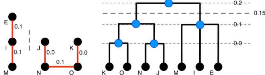
Given a dendogram, a single segmentation of the image can be obtained very easily, by cutting the dendogram at a fixed altitude, or threshold. After cutting the dendogram at a fixed altitude, we are left with a set of subtrees, called connected components. These connected components cover the original image (i.e. each node in the original graph belongs to one and only one component), and represent a possible segmentation of the image. Intuitively, if the original edge weighting function is a simple Euclidean distance between neighbors, that segmentation is very brittle, as it depends on very local edge information.

0.1 0.0 0.0 0.1 0.1 E I J K M N O 0.15 K O N J M I 0.1 0.0 0.2 E

Figure 1.6: Cutting the Dendogram = Segmenting - Left: two connected compo-nents, obtained after thresholding at 0.15. Right: dendogram of MST, any node above the threshold will be removed. the graph.

Alternatively, the dendogram can be filtered, according to criterions that depend on the geometry of the underlying component (surface, volume, . . . ). Felzenszwalb & Huttenlocher (35) proposed an interesting method to produce final components, using a criterion that compares the maximum weight within a component to each edge between any two components, and have an adaptive threshold that depends on this ratio. The method produces balanced segmentations which are robust to local noise. This type of technique effectively performs a non-horizontal cut of the hierarchy, taking into account the local morphology of each subtree.

More advanced forms of thresholding criteria can even involve learning. This can be achieved by defining a function over a neighborhood of pixels, to produce the edge costs in such a way that graph-cut segmentation and similar methods produce the best answer. One such objective function is Turaga’s Maximin Learning (100), which pushes up the lowest edge cost along the shortest path between two points in different segments, and pushes down the highest edge cost along a path between two points in the same segment.

In this thesis I was mostly interested in using segmentation hierarchies to explore a large set of candidate segmentations in an efficient way. The focus of the thesis is thus more on the use of such trees, as complements to feature learners, rather than on their production.

1.2.2 Structured Prediction

Structured prediction is a term that describes techniques that involve predicting struc-tured objects, i.e.considering output labels as inter-dependent, and explicitly modeling this inter-dependence. One of the earliest structured prediction systems was proposed

by LeCun et al. (65), to address the problem of labeling scanned documents. The challenge there is that there is a joint problem of segmentation and recognition: given a long bitmap of characters, one must jointly find the best segmentation into charac-ters and classify each character. Any problem that involves labeling sequence data can be treated with the technique proposed in (65): speech recognition, natural language processing, handwritten text recognition (OCR), music transcription. . .

For sequence data, one can easily produce all possible segmentations, and compute a unary cost for each segment. The Viterbi algorithm can then be used to find the most likely sequence of labels.

For image labeling problems, segmentation becomes problematic, as there is no way to exhaustively explore all possible segmentation candidates: the graph being loopy, decoding has to be done in an approximate way, using techniques like loopy belief-propagation, or graph cuts.

1.2.2.1 Graphical Models

Let us start with a general introduction of undirected graphical models for structured prediction tasks. We assume a graph G = (V, E) with vertices i ∈ V and edges e ∈ E ⊆ V × V . The joint probability of a particular assignment to all the variables xi is represented as a normalized product of a set of non-negative potential functions:

p(x1, x2, . . . , x|V |) = 1 Z Y i∈V φi(xi) Y ejk∈E φejk(xj, xk). (1.15)

There is one node potential function φi for each node i, and one edge potential φe for each edge e. Each edge connects two nodes, ej and ek. In a complete graph, there is one edge between each possible pair of nodes. For common applications, such as computer vision, it’s much more common to have locally connected graphs, i.e. graphs in which only (small) subsets of nodes are connected via edges (see previous section).

The node potential function φi gives a non-negative weight to each possible value of the random variable xi. For example, we might set φi(xi= 0) to 0.75 and φi(xi = 1) to 0.25, which means means that node i has a higher potential of being in state 0 than state 1. Similarly, the edge potential function φejk gives a non-negative weight to all

The normalization constant Z, or partition function, is a scalar value that forces the distribution to sum to one, over all possible joint configurations of the variables:

Z =X x1 X x2 · · ·X x|V | Y i∈V φi(xi) Y ejk∈E φejk(xj, xk). (1.16)

This normalizing constant ensures that the model defines a valid probability distri-bution.

Given a graph G, there are three tasks that are commonly performed:

• parameter estimation (learning): the task of computing the potential functions φ that maximize the likelihood of the training data (or, given a predefined function φ parametrized by W, finding the optimal parameters W);

• inference: the task of estimating the partition function Z as well as the marginal probabilities of each node taking each possible state;

• decoding: the task of finding the most likely joint configuration of the variables (the configuration that has the highest joint probability).

1.2.2.2 Learning: Parameter Estimation

As explained in Section 1.1, if we are only interested in discrimination (classification), Graphical models can be simplified by considering the negative log likelihood, and ig-noring the normalization constant Z (which quickly becomes intractable and/or mean-ingless for large problems). We define the energy E ∝ − log(p):

E(x1, x2, . . . , x|V |) = X i∈V Φi(xi) + X ejk∈E Φejk(xj, xk). (1.17)

We assume that Φi and Φe are predefined functions (a linear model, a multilayer perceptron, or a convolutional network), parametrized by a set of trainable weights w. For stationary data (images, audio. . . ), it is common to have models that are fixed across locations, and that only depend on their input xi and the groundtruth label ti. Since they are constant across locations, we can drop the subscripts i and e, and rename them φ and ψ, which are now functions of xi, ti and w. We can rewrite the energy as: E(x, t; w) =X i∈V Φ(xi, ti; wφ) + X ejk∈E Ψejk(xj, xk, tj, tk; wψ), (1.18)

where x is the vector of input nodes, and t is the vector of groundtruth labels for each node. This energy is also known as the Conditional Random Field (CRF) energy.

The parameter estimation task (learning) becomes a simple minimization problem, similar to that described in Section 1.1. Reusing the same formulation, and assuming a training set of pairs {xn, yn} ∀ n ∈ {1, . . . , N }, we have:

l(φ, ψ; xn, tn, w) = E(xn, tn; w) ∀ n ∈ {1, . . . , N } (1.19) L(φ, ψ; x, t, w) = X

n∈{1,...,N }

l(f ; xn, tn, w). (1.20)

Depending on the forms of φ and ψ, the overall objective L might be convex or not. In the classical CRF literature, the potential functions are usually linear in their parameters, so the overall problem is indeed convex. Optimization details presented in Section 1.1.2.2 also apply here. In particular, stochastically estimating the gradients can tremendously accelerate the learning, as opposed to using more exact methods like L-BFGS.

More generally, the potential functions can be arbitrarily complex non-convex func-tions, for example, in the case of image labeling they could be full-blown convolutional networks, which depend on a neighborhood of input variables. In this case, the over-all objective function becomes non-convex, and the learning problem chover-allenging. A simpler solution is to modularize the process of learning, and do it in two steps: (1) train the unary potentials (the convolutional network) on individual input samples; (2) freeze the unary potential functions, pre-compute them for all images, and learn the CRF parameters (a convex problem). That second approach is the basis of Chapter 2. One of the central results of this thesis is the fact that using a powerful node potential, such as a multiscale convolutional network (as presented in Chapter 2), can greatly reduce the need for a top down, global CRF, as each node potential manages to learn the structure of a large set of input variables.

1.3

Dataflow Computing

The third contribution of this thesis is a custom dataflow computer architecture op-timized for the computation of convolutional networks (such as the model presented in Section 2). Dataflow computers are a particular type of processing architecture, which aim at maximizing the number of effective operations per instruction, which in

turn maximizes the number of operations reachable per second and per watt consumed. They are particularly well fit to the computation of convolutional networks, as these require very little branching logic, and rather require tremendous quantities of basic, redundant arithmetic operations.

In this section I provide a very quick primer on dataflow computing and architec-tures. As I suspect most readers of this thesis will come from a software background, this section is rather high-level, with an emphasis on the compute model rather than on the specific details of implementation. Chapter 3 extensively describes our custom dataflow architecture.

Dataflow architectures are a particular type of computer architecture that directly contrasts the traditional von Neumann architecture or control flow architecture. Data-flow architectures do not have a program counter, or (at least conceptually) the execu-tion of instrucexecu-tions is solely determined based on the availability of input data to the compute elements.

Dataflow architectures have been successfully implemented in specialized hardware such as in digital signal processing (3, 85), network routing (5), graphics processing (71, 92). It is also very relevant in many software architectures today including database engine designs and parallel computing frameworks (9, 10).

Before getting into the details of the dataflow architecture, let us look at the Von Neumann architecture, which should help highlight the fundamental shortcomings of traditional flow control for highly data-driven applications.

In this type of architecture, the control unit, which decodes the instructions and executes them, is the central point of the system. A program (sequence of instructions) is typically stored in external memory, and sequentially read into the control unit. Certain types of instructions involve branching, while others involve reading data from the memory into the arithmetic logic unit (ALU), to transform them, and write them back into external memory.

When executing programs that are highly unpredictable in terms of branching (pro-grams that have many possible execution paths, with an essentially uniform probability distribution), this type of architecture is optimal. The control unit loads one instruc-tion per clock cycle, which either: (1) reads data into the ALU, (2) writes it back to memory, (3) triggers an ALU operation on data that are already in local registers, or

compute logic. When the data streams into the compute logic, computations occur continuously, and the processed data can be saved back into memory. There is no fine grained, cycle-accurate control, rather the flows of data themselves trigger the computations.

The core of the architecture proposed in this thesis relies on this idea of data-driven computations, complemented by a powerful online hardware re-configuration system, and a global, macroscopic control flow unit. Figure 1.8 provides an overview of this architecture.

The most striking aspect of this architecture is the ratio between actual compute logic and control+caching logic. Caching is essentially nil, as the entire architecture is designed to work on streams: as the streams produce the computations, there is no need for caching (there is no latency to hide, as the control unit works asynchronously). The control logic is very sparse in its activity, as it is only here to reconfigure the grid of processing tiles (PTs on the figure): before scheduling any new computation, it configures multiple tiles to perform given operations, and it also configures all the routes/connections between tiles and global data paths. Once the grid is configured, streams of data can come into it, and produce thousands, or millions of results, before a new configuration is required. Configurations can be initiated in parallel with the computations.

The Processing Tiles (PTs) are passive computers. Each tile can be configured to do one of several basic arithmetic tasks (including common DSP functions, like dot products, and convolutions).

❳ ✰ ✪ ▼ ✁✂ ❳ ✰ ✪ ▼ ✁✂ ❳ ✰ ✪ ▼ ✁✂ ❳ ✰ ✪ ▼ ✁✂ ❳ ✰ ✦✄ ✪ ▼ ✁✂ ❳ ✰ ✪ ▼ ✁✂ ❳ ✰ ✪ ▼ ✁✂ ❳ ✰ ✪ ▼ ✁✂ ❳ ✰ ✪ ▼ ✁✂ ❈☎ ✆✝✞☎ ✟ ✥❈☎ ✆✠✡☛ ❙☞✌✞✝✍▼ ✎ ✏✑ ✒ ✓✔ ✕ ✖✗ ✘ ✙✚ ✛✜✑✖✢✛ ●✚ ✑ ✙✘✚✣✘ ✢ ✘▲✔ ✒✛s ✜ ✖ ✒✢ ✔ ❘✛✏✑✒✓✔ ✕✤ ✖s ❖ ✠✠❢✧ ★✡ ✩ ▼ ✫ ☞☎✞✬ ✭ ✮✯ ✦✄ ✭ ✮✯ ✦✄ ✭✮✯ ✦✄ ✭ ✮✯ ✦✄ ✭ ✮✯ ✦ ✄ ✭✮✯ ✦✄ ✭✮✯ ✦✄ ✭✮✯ ✦✄ ✭ ✮✯ ❆✱✉♥ t✐♠ ❡✱❡❝ ♦♥✲✐ ❣✉ r❛❜ ❧❡❉❛ t❛✲ ❧♦✇❆ r❝ ❤✐t❡❝t✉ r❡ P ✳ P ✳ P ✳ P✳ P ✳ P ✳ P ✳ P ✳ P ✳

Figure 1.8: Our Proposed Dataflow Architecture - Diagram of our dataflow archi-tecture.

Image Understanding: Scene

Parsing

2.1

Introduction

Image understanding is a task of primary importance for a wide range of practical applications. One important step towards understanding an image is to perform a full-scene labeling also known as a full-scene parsing, which consists in labeling every pixel in the image with the category of the object it belongs to. After a perfect scene parsing, every region and every object is delineated and tagged. One challenge of scene parsing is that it combines the traditional problems of detection, segmentation, and multi-label recognition in a single process.

There are two questions of primary importance in the context of scene parsing: how to produce good internal representations of the visual information, and how to use contextual information to ensure the self-consistency of the interpretation.

2.2

A Model for Scene Understanding

2.2.1 Introduction

This chapter presents a scene parsing system that relies on deep learning methods to approach both questions. The main idea is to use a convolutional network (65) operating on a large input window to produce label hypotheses for each pixel location. The convolutional net is fed with raw image pixels (after band-pass filtering and contrast

normalization), and trained in supervised mode from fully-labeled images to produce a category for each pixel location. Convolutional networks are composed of multiple stages each of which contains a filter bank module, a non-linearity, and a spatial pooling module. With end-to-end training, convolutional networks can automatically learn hierarchical feature representations.

Unfortunately, labeling each pixel by looking at a small region around it is difficult. The category of a pixel may depend on relatively short-range information (e.g. the presence of a human face generally indicates the presence of a human body nearby), but may also depend on long-range information. For example, identifying a grey pixel as belonging to a road, a sidewalk, a gray car, a concrete building, or a cloudy sky requires a wide contextual window that shows enough of the surroundings to make an informed decision. To address this problem, we propose to use a multi-scale convo-lutional network, which can take into account large input windows, while keeping the number of free parameters to a minimum.

Common approaches to scene parsing first produce segmentation hypotheses using graph-based methods. Candidate segments are then encoded using engineered features. Finally, a conditional random field (or some other type of graphical model), is trained to produce labels for each candidate segment, and to ensure that the labelings are globally consistent.

A striking characteristic of the system proposed here is that the use of a large con-textual window to label pixels reduces the requirement for sophisticated post-processing methods that ensure the consistency of the labeling.

More precisely, the proposed scene parsing architecture is depicted on Figure 2.1. It relies on two main components:

1) Multi-scale, convolutional representation: our multi-scale, dense feature extractor produces a series of feature vectors for regions of multiple sizes centered around every pixel in the image, covering a large context. The multi-scale convolutional net contains multiple copies of a simple network (all sharing the same weights) that are applied to different scales of a Laplacian pyramid version of the input image. For each pixel, the networks collectively encode the information present in a large contextual window around the given pixel (184 × 184 pixels in the system described here). The convolutional network is fed with raw pixels and trained end to end, thereby alleviating

2.b. Conditional random field over superpixels: a conditional random field is defined over a set of superpixels. Compared to the previous, simpler method, this post-processing models joint probabilities at the level of the scene, and is useful to avoid local aberrations (e.g. a person in the sky). That kind of approach is widely used in the computer vision community, and we show that our learned multiscale feature representation essentially makes the use of a global random field much less useful: most scene-level relationships seem to be already captured by it.

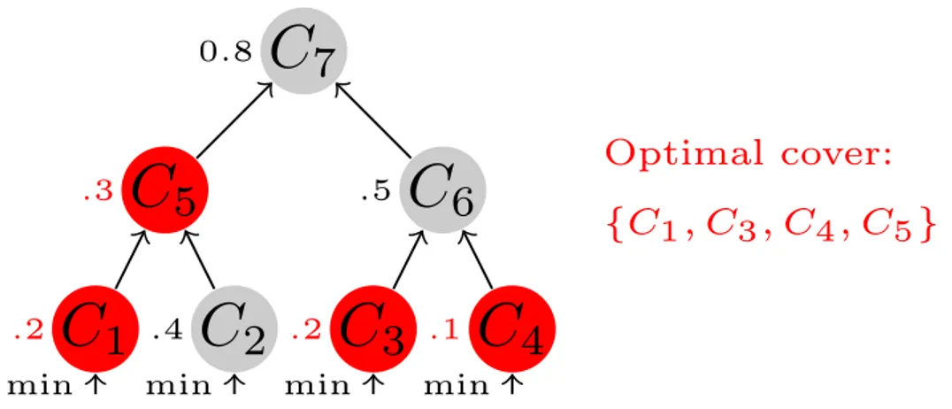
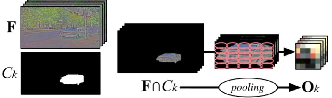
2.c. Multilevel cut with class purity criterion: A family of segmentations is constructed over the image to analyze the scene at multiple levels. In the simplest case, this family might be a segmentation tree; in the most general case it can be any set of segmentations, for example a collection of superpixels either produced using the same algorithm with different parameter tunings or produced by different algorithms. Each segmentation component is represented by the set of feature vectors that fall into it: the component is encoded by a spatial grid of aggregated feature vectors. The ag-gregated feature vector of each grid cell is computed by a component-wise max pooling of the feature vectors centered on all the pixels that fall into the grid cell. This pro-duces a scale-invariant representation of the segment and its surrounding. A classifier is then applied to the aggregated feature grid of each node. This classifier is trained to estimate the histogram of all object categories present in the component. A subset of the components is then selected such that they cover the entire image. These com-ponents are selected so as to minimize the average “impurity” of the class distribution in a procedure that we name “optimal cover”. The class “impurity” is defined as the entropy of the class distribution. The choice of the cover thus attempts to find a con-sistent overall segmentation in which each segment contains pixels belonging to only one of the learned categories. This simple method allows us to consider full families of segmentation components, rather than a unique, predetermined segmentation (e.g. a single set of superpixels).

All the steps in the process have a complexity linear (or almost linear) in the num-ber of pixels. The bulk of the computation resides in the convolutional network feature extractor. The resulting system is very fast, producing a full parse of a 320 × 240 image in less than a second on a conventional CPU, and in less than 100ms using dedicated

hardware, opening the door to real-time applications. Once trained, the system is pa-rameter free, and requires no adjustment of thresholds or other knobs.

An early version of this work was first published in (34). This journal version reports more complete experiments, comparisons and higher results.

2.2.2 Multiscale feature extraction for scene parsing

The model proposed in this chapter, depicted on Figure 2.1, relies on two complemen-tary image representations. In the first representation, an image patch is seen as a point in RP, and we seek to find a transform f : RP → RQ that maps each patch into RQ, a space where it can be classified linearly. This first representation typically suffers from two main problems when using a classical convolutional network, where the image is divided following a grid pattern: (1) the window considered rarely contains an object that is properly centered and scaled, and therefore offers a poor observation basis to predict the class of the underlying object, (2) integrating a large context in-volves increasing the grid size, and therefore the dimensionality P of the input; given a finite amount of training data, it is then necessary to enforce some invariance in the function f itself. This is usually achieved by using pooling/subsampling layers, which in turn degrades the ability of the model to precisely locate and delineate objects. In this chapter, f is implemented by a multiscale convolutional network, which allows integrating large contexts (as large as the complete scene) into local decisions, yet still remaining manageable in terms of parameters/dimensionality. This multiscale model, in which weights are shared across scales, allows the model to capture long-range in-teractions, without the penalty of extra parameters to train. This model is described in Section 2.2.2.1.

In the second representation, the image is seen as an edge-weighted graph, on which one or several over-segmentations can be constructed. The components are spatially ac-curate, and naturally delineate the underlying objects, as this representation conserves pixel-level precision. Section 2.2.3 describes multiple strategies to combine both repre-sentations. In particular, we describe in Section 2.2.3.3 a method for analyzing a family of segmentations (at multiple levels). It can be used as a solution to the first problem exposed above: assuming the capability of assessing the quality of all the components

in this family of segmentations, a system can automatically choose its components so as to produce the best set of predictions.

2.2.2.1 Scale-invariant, scene-level feature extraction

Good internal representations are hierarchical. In vision, pixels are assembled into edglets, edglets into motifs, motifs into parts, parts into objects, and objects into scenes. This suggests that recognition architectures for vision (and for other modalities such as audio and natural language) should have multiple trainable stages stacked on top of each other, one for each level in the feature hierarchy. Convolutional Networks (ConvNets) provide a simple framework to learn such hierarchies of features.

Convolutional Networks (64, 65) are trainable architectures composed of multiple stages. The input and output of each stage are sets of arrays called feature maps. For example, if the input is a color image, each feature map would be a 2D array containing a color channel of the input image (for an audio input each feature map would be a 1D array, and for a video or volumetric image, it would be a 3D array). At the output, each feature map represents a particular feature extracted at all locations on the input. Each stage is composed of three layers: a filter bank layer, a non-linearity layer, and a feature pooling layer. A typical ConvNet is composed of one, two or three such 3-layer stages, followed by a classification module. Because they are trainable, arbitrary input modalities can be modeled, beyond natural images.

Our feature extractor is a three-stage convolutional network. The first two stages contain a bank of filters producing multiple feature maps, a point-wise non-linear map-ping and a spatial pooling followed by subsampling of each feature map. The last layer only contains a bank of filters. The filters (convolution kernels) are subject to training. Each filter is applied to the input feature maps through a 2D convolution operation, which detects local features at all locations on the input. Each filter bank of a convo-lutional network produces features that are equivariant under shifts, i.e. if the input is shifted, the output is also shifted but otherwise unchanged.

While convolutional networks have been used successfully for a number of image labeling problems, image-level tasks such as full-scene understanding (pixel-wise label-ing, or any dense feature estimation) require the system to model complex interactions at the scale of complete images, not simply within a patch. To view a large contextual