Laboratoire d'Analyse et Modélisation de Systèmes pour l'Aide à la Décision CNRS UMR 7024
CAHIER DU LAMSADE
290
Decembre 2009
The two-machine flow-shop serial-batching
scheduling problem with limited batch size
M. A. ALOULOU, A. BOUZAIENE, N. DRIDI,
D. VANDERPOOTEN
The two-machine flow-shop serial-batching scheduling problem
with limited batch size
Mohamed Ali Aloulou1, Afef Bouzaiene1,2, Najoua Dridi2, and Daniel Vanderpooten1 1LAMSADE, Universit´e Paris Dauphine, France
(aloulou,bouzaiene,vdp)@lamsade.dauphine.fr 2OASIS - Ecole Nationale d’Ing´enieurs de Tunis, Tunisia
Abstract
We consider the the two-machine flow-shop serial-batching scheduling problem where the batches have limited size. Two criteria are considered here. The first criterion is to minimize the number of batches. This criterion reflects situations where processing of any batch induces a fixed cost, which leads to a total cost proportional to the number of batches. The second criterion is the makespan. We study the complexity of the problem and propose polynomial-time algorithms for some particular cases and an approximation algorithm with a guaranteed performance for the general case.
Keywords: two-machine flow-shop, serial batching, limited batch size, makespan, batch cost.
1
Problem formulation and motivation
The following two-machine flow-shop scheduling problem is considered. We have a set of n jobs to be processed. Each job i, i = 1, . . . n, is made up of two operations. The first operation is handled on machine M1 and its processing time is denoted by ai. The second operation is
handled on machine M2 and its processing time is denoted by bi. M1 and M2 are two
serial-batch (or sum-serial-batch) machines with a limited capacity, denoted by c, in terms of the number of jobs (each job i has a unit size si= 1). The following assumptions are made: (i) preemption
is not allowed, (ii) each batch in both machines does not contain more than c operations, (iii) operations within a batch can be processed in any order, (iv) the total processing time of a batch is equal to the sum of the processing times of the operations in the batch, (v) an operation is assumed to be completed if all the operations in its batch are completed (batch availability constraint). Two criteria are considered here. The first criterion is to minimize the number of batches #batch. This criterion reflects situations where processing of any batch induces a fixed cost, which leads to a total cost proportional to #batch. The second criterion is the makespan Cmax, i.e. the completion time of the last job on machine M2. This bicriteria
scheduling problem is denoted by F 2|sum-batch, c|(#batch, Cmax).
Our model can be seen as a generalization of the model proposed by [1], where the authors studied the problem of finding group-schedules for problem F 2||Cmax. A group-schedule is
conflicting criteria are of interest: flexibility of a solution and its makespan. The flexibility is measured by the number of batches in the solution and the makespan is computed as for serial-batch models. The only difference with our model is that the number of jobs in a batch is not limited, i.e. c = n. Referring to previous results of [2] for F 2|sum-batch|Cmax (with
setup times), they conclude that the constrained problems F 2|sum-batch, Cmax ≤ α|#batch
and F 2|sum-batch, #batch = k|Cmax are NP-hard in the strong sense. When k is fixed,
the second problem is NP-hard in the ordinary sense. They also provide polynomial-time approximation algorithms for these problems. Unfortunately, these algorithms cannot be extended to our model.
If the number of jobs n is a multiple of c, i.e. n = ch, then the solution with a minimum number of batches contains exactly h full batches. Here, a batch is called full if it contains exactly c jobs. The lexicographic bicriteria problem F 2|sum-batch, c|Lex(#batch, Cmax) is
equivalent to problem F 2|sum-batch, c-in-1|Cmax, where notation c-in-1 imposes to have
ex-actly c jobs in a batch insuring that the number of batches is minimum. This notation has been first introduced by [3] for single-machine batch scheduling. The authors considered prob-lem 1|sum-batch, c-in-1, wi = pi|P wiCi and proved that it is NP-hard in the strong sense
when c ≥ 3 and polynomially solvable when c = 2. They also provide a polynomial time algorithm when the jobs are inversely agreeable, i.e. pi< pj implies wi ≥ wj.
If the number of jobs is not multiple of c, we can add c × dnce − n dummy jobs with zero processing times in both machines and solve problem F 2|sum-batch, c-in-1|Cmaxto determine
the solution minimizing the makespan under the constraint that the number of batches is minimum. By the same way, if we impose a number of batches #b ∈ {dnce, . . . , n}, in order to determine a solution with minimum makespan, we add c × #b − n dummy jobs with zero processing time in both machines and solve problem F 2|sum-batch, c-in-1|Cmax. Hence,
solving (n − dBne + 1) times problem F 2|sum-batch, c-in-1|Cmax allows us to solve problem F 2|sum-batch, c|(#batch, Cmax).
In this paper, we first study the complexity of problem F 2|sum-batch, c-in-1|Cmax. Then
we propose polynomitime algorithms for some particular cases and an approximation al-gorithm with a guaranteed performance for the general case.
2
Complexity
Theorem 1 Problem F 2|sum-batch, c-in-1|Cmax is NP-hard in the strong sense for c ≥ 3,
even if ai= bi for all i = 1, . . . , n.
Proof : First remark that in this case all batches have the same duration on both machines and consequently if the batches are formed the makespan of any batch sequence is equal to the sum of ai, i = 1, . . . , n plus the duration of the largest batch. Hence to solve problem
F 2|sum-batch, c-in-1, ai = bi|Cmax, we only have to constitute the batches such that the
duration of the largest one is minimum.
We use a polynomial transformation from the 3-Partition problem: Given 3m + 1 positive integers c1, . . . , c3m and C such that C/4 < cj < C/2, j = 1, . . . , 3m, and P3mj=1cj = mC, is
there a partition of the set {1, . . . , 3m} into m subsets X1, . . . , Xm, for which Pj∈Xlcj = C,
l = 1, . . . , m? Given an instance of this problem, construct the following instance of our problem. There are 3m jobs i such that ai = bi = ci. We show that 3-partition problem
has a solution if, and only if, there exists a solution to the constructed instance such that #batch = m and Cmax≤ y := (m + 1)C.
Suppose that 3-partition problem has a solution X = {X1, . . . , Xm}. Constitute m batches
according to solution X. The makespan of any batch sequence is equal to P
j=1,...,mXj +
maxj=1,...,mXj = mC + C = (m + 1)C.
Assume now that there exists a schedule such that #batch = m and Cmax≤ (m+1)C. Let
X1, . . . , Xm be the duration of the corresponding batches. We have Cmax= Pj=1,...,mXj+
maxj=1,...,mXj = mC + maxj=1,...,mXj ≤ (m + 1)C. Then maxj=1,...,mXj = C and X1 =
. . . = Xm= C, which means that X = {X1, . . . , Xm} is solution to 3-partition problem.
However, problem F 2|sum-batch, 2-in-1|Cmax is open.
3
Polynomial-time cases
Solving the batching problem for a given job sequence: Given a job sequence π, we propose a polynomial-time dynamic-programming algorithm, named DP 1(π), allowing us to solve the bicriteria problem F 2|sum-batch, c|(#batch, Cmax), i.e. determine the Pareto
optimal solutions set Eπ subject to the constraint that the jobs follow sequence π. We first
renumber the jobs according to sequence π. For each partial solution in which we have already scheduled i jobs, we associate a state(i, k, q), where k is the total number of jobs in the last batch and q is the number of batches. Let C(i, k, q) denote the minimum makespan among all partial solutions corresponding to the same state state(i, k, q). Algorithm DP 1(π) recursively calculates values C(.). The initialization is given by :
C(i, k, q) = ∞ (i = 0, ..., n; k = 0, ..., n, q = 0, ..., n.) and C(0, 0, 0) = 0. The recursion for i = 1, ..., n, k = 1, ..., i and q = 1, ..., i is given by: C(i, k, q) = ∞, if k > c, max(C(i − 1, k − 1, q) −Pk−1 j=1bi−j, Pi j=1aj) + Pk−1 j=0bi−j, if 1 < k ≤ c,
minp=0,...,i−1{max(C(i − 1, p, q − 1),Pij=1aj)) + bi}, if k = 1.
In order to enumerate all Pareto optimal solutions following the given sequence, we determine, for each value q ∈ {1, ..., n}, the optimal makespan, which is given by mink=1,...,nC(n, k, q). The corresponding solutions are obtained by backtracking. The
run-ning time of algorithm DP 1(π) can be evaluated as O(n3).
Equal processing times and batches of size two: We consider here the problem F 2|sum-batch, 2 − in − 1, ai= bi|Cmax. First renumber the jobs such that a1 ≤ a2 ≤ ... ≤ an.
We have the following results.
Lemma 1 If n is even, then there exists an optimal solution for problem F 2|sum-batch, 2-in-1, ai = bi|Cmax in which jobs i and (n − i + 1), for i = 1, . . . , n/2,
are in the same batch.
Proof : Consider an optimal solution π characterized by batches B1, . . . , Bh (with h = n/2).
Suppose that jobs 1 and n are not in the same batch, i.e. job 1 is with some job j1 in a
batch Bk and job n is with another job j2 in a batch Bl. Construct a new solution π0 in
which jobs 1 and n are in the same batch Bk0, jobs j1 and j2 are in the same batch Bl0, and
the other batches are the same as in π. Denote by p(Br) =Pi∈Brai, r = 1, . . . , h. We have
p(B0k) = a1+ an≤ aj2+ an= p(Bl) and p(B
0
maxr=1,...,hp(Br0) ≤ maxr=1,...,hp(Br) and we have Cmax(π0) ≤ Cmax(π), which means that π0
is also optimal. By repeating the same procedure at most n/2 times, we obtain a solution satisfying the property.
If the number of jobs is odd, we can easily prove that job n is alone on a batch and jobs i and (n − i), for i = 1, . . . , bn/2c, are in the same batch. Hence, we get the following result. Theorem 2 Problem F 2|sum-batch, 2-in-1, ai = bi|Cmax can be solved in O(n log n) time.
As a consequence, problem F 2|sum-batch, c = 2, ai = bi|(#batch, Cmax) can be solved
in O(n2) time by adding some dummy jobs and solve O(n) 2-in-1 problems. Remark that imposing a number of batches #b, n/2 ≤ #b ≤ n, implies that there are (2 × #b − n) batches with one job each and (n − #b) batches containing each 2 jobs. In an optimal solution, the latter batches will contain the jobs with largest processing time, i.e. jobs (2n−2#b+1), . . . , n, and the former batches are constructed according to lemma 1. Consequently, we have the following result.
Corollary 1 The bicriteria problem F 2|sum-batch, c = 2, ai = bi|(#batch, Cmax) can be
solved in O(n2) time.
Constant processing time for the first or the second machine: We can prove the following result by the job interchange argument.
Lemma 2 Any Pareto optimal solution of problem F 2|sum-batch, c, ai = a|(#batch, Cmax)
can be transformed into a solution with the same performance measure values such that the jobs are processed in LPT order with respect to their processing times on machine M2.
Using algorithm DP 1(πLP T (M2)), we get the following result.
Theorem 3 F 2|sum-batch, c, ai = a|(#batch, Cmax) can be solved in O(n3) time.
Similarly, we can prove that any Pareto optimal solution of problem F 2|sum-batch, c, bi=
b|(#batch, Cmax) can be transformed into a solution with the same performance measure
values such that the jobs are processed in SPT order with respect to their processing times on machine M1. Using algorithm DP 1(πSP T (M1)) allows to solve the problem.
Theorem 4 F 2|sum-batch, c, bi = b|(#batch, Cmax) can be solved in O(n3) time.
4
A polynomial-time approximation algorithm
We consider here that the number of jobs n is such that n = ch, h > 0. Otherwise, we add (ch − bn/cc) dummy jobs with zero processing times in both machines. We propose an approximation algorithm, named A(c), to solve problem F 2|sum-batch, c-in-1|Cmax in
polynomial time when c is constant. In this algorithm, batches are formed according to Johnson sequence. When the condition in instruction 6 is not verified, and when h ≥ 2c − 2, jobs of batch Bk are separated and mixed with the jobs of the following (or previous) c − 1
Algorithm 1: Algorithm A(c)
Number the jobs according to Johnson sequence πJ = (1, 2, . . . ch)
1
Compute CmaxJ the optimal makespan of the F 2||Cmax problem 2
Group jobs into h batches of c jobs according to sequence πJ to form solution
3
S = (B1, . . . , Bh)
Compute the makespan Cmax(S) of solution S 4
Identify a batch Bk such thatPcki=1ai+Pchi=c(k−1)+1bi = Cmax(S) 5
if min0≤t≤c−1{Pcki=c(k−1)+2+tai+Pc(k−1)+ti=c(k−1)+1bi} ≤ C
J max 2 then 6 Return solution S 7 else 8 if h ≥ 2c − 2 then 9 if 1 ≤ k ≤ c − 1 then 10 for r ← 0 to c − 1 do 11
Replace batch Bk+r by batch Bk+r0 = (c(k − 1) + 1 + r, i2r, . . . , icr) where 12
ilr= c(k + r) − r − 1 + l, l = 2, . . . , c Return the resulting solution
13 S0 = (B1, . . . , Bk−1, Bk0, . . . , Bk+c−10 , Bk+c, . . . , Bh) else 14 for r ← 0 to c − 1 do 15
Replace batch Bk−c+1+r by batch 16
Bk−c+1+r00 = (c(k − 1) + 1 + r, jr2, . . . , jrc) where jrl = c(k − c + r) − r − 1 + l, l = 2, . . . , c Return the resulting solution
17
S00= (B1, . . . , Bk−c, Bk−c+100 , . . . , Bk00, Bk+1, . . . , Bh)
else
18
Select and return a best solution among all possible solutions
19
Theorem 5 Algorithm A(c) is a polynomial-time approximation algorithm for problem F 2|sum-batch, c-in-1|Cmax with tight approximation ratio ρ = 32 when c is constant.
Proof : Denote by Cmax∗b the optimal makespan for problem F 2|sum-batch, c-in-1|Cmax.
In algorithm A(c) batch Bk defines Cmax(S), then we have Cmax(S) =
Pck i=1ai +
Pch
i=c(k−1)+1bi that can be rewritten, for all t = 0, . . . , c − 1,
Cmax(S) = c(k−1)+1+t X i=1 ai+ ch X i=c(k−1)+1+t bi+ ck X i=c(k−1)+2+t ai+ c(k−1)+t X i=c(k−1)+1 bi. (1) Hence, we have
Cmax(S) ≤ CmaxJ +t=0,...,c−1min { ck X i=c(k−1)+2+t ai+ c(k−1)+t X i=c(k−1)+1 bi}. (2)
Consequently, if min t=0,...,c−1{ ck X i=c(k−1)+2+t ai+ c(k−1)+t X i=c(k−1)+1 bi} ≤ 1 2C J max,
then Cmax(S) ≤ 32CmaxJ ≤ 32C ∗b
max. (instructions 6 and 7 in the algorithm).
Otherwise, since CmaxJ ≥Pl
i=1ai+ Pch i=lbi, l = 1, . . . , ch, we get ∀l = 1, . . . , c(k − 1) + 1, ck, . . . , ch, l X i=1 i6∈Bk\{c(k−1)+1} ai+ ch X i=l i6∈Bk\{ck} bi < 1 2C J max. (3)
We distinguish two cases:
1. Case where 1 ≤ k ≤ c − 1. Algorithm A(c) provides solution S0 (see instructions 11-13). Let Bl0 be the batch determining the makespan of solution S0. Then:
• if l < k or l ≥ k + c then Cmax(S0) = cl X i=1 ai+ ch X i=c(l−1)+1 bi = cl X i=1 ai+ ch X i=cl bi+ cl−1 X i=c(l−1)+1 bi
According to equations (3), we have Pcl−1
i=c(l−1)+1bi < 12CmaxJ . Then,
Cmax(S0) ≤ 32CmaxJ ≤ 32C ∗b max. • if k ≤ l ≤ k + c − 1, let l = k + r, 0 ≤ r ≤ c − 1. We have Cmax(S0) = c(k−1) X i=1 ai + ac(k−1)+1+ ai2 0 + . . . + ai c 0 + . . . + ac(k−1)+1+r + ai2 r + . . . + aicr + bc(k−1)+1+r+ bi2 r+ . . . + bicr + . . . + bck+ bi2 c−1 + . . . + bi c c−1 + ch X i=c(k+c−1)+1 bi
Hence, we have the following Cmax(S0) = c(k−1)+1+r X i=1 ai+ ic r X i=i2 0 ai+ ch X i=c(k−1)+1+r bi− icr−1 X i=i2 0 bi. (4)
According to equations (3), we have Picr
i=i2 0ai <
1
2CmaxJ . Then, Cmax(S0) ≤ 3 2C J max≤ 32C ∗b max.
2. Case where k ≥ c. Algorithm A(c) provides solution S00(see instructions 15-17) Let B00l be the batch determining the makespan of solution S00. Then:
• if l ≤ k − c or l > k then Cmax(S00) = cl X i=1 ai+ ch X i=c(l−1)+1 bi = cl X i=1 ai+ ch X i=cl bi+ cl−1 X i=c(l−1)+1 bi
According to equations (3), we have Pcl−1
i=c(l−1)+1bi < 12CmaxJ . Then,
Cmax(S00) ≤ 32CmaxJ ≤ 32C ∗b max. • if k − c + 1 ≤ l ≤ k, let l = k − c + 1 + r, 0 ≤ r ≤ c − 1. We have Cmax(S00) = c(k−c) X i=1 ai + ac(k−1)+1+ aj2 0 + . . . + aj c 0 + . . . + ac(k−1)+1+r+ aj2 r + . . . + ajrc + bc(k−1)+1+r+ bj2 r + . . . + bjrc + . . . + bck+ bj2 c−1+ . . . + bj c c−1 + ch X i=ck+1 bi
Hence, we have the following Cmax(S00) = c(k−1)+1+r X i=1 ai+ ch X i=c(k−1)+1+r bi+ jc c−1 X i=j2 r bi− jc c−1 X i=j2 r+1 ai. (5)
According to equations (3), we have Pjcc−1
i=j2 rbi <
1
2CmaxJ . Then, Cmax(S00) ≤ 3
2CmaxJ ≤ 32C ∗b max.
If h < 2c − 2, then we select a best solution, with makespan equal to Cmax∗b among all possible solutions (instruction 19 in the algorithm). The number of all possible solutions is less than (2c(c − 1))! that is polynomial since c is constant.
To summarize, in all cases algorithm A(c) provides a solution with a makespan less or equal to 32Cmax∗b .
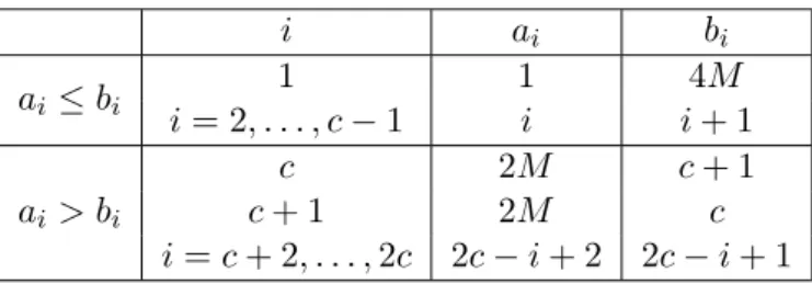
Table 1: An example with a ratio equal to 3/2 i ai bi ai ≤ bi 1 1 4M i = 2, . . . , c − 1 i i + 1 ai > bi c 2M c + 1 c + 1 2M c i = c + 2, . . . , 2c 2c − i + 2 2c − i + 1
In order to prove that the approximation ratio is tight, consider the following instance composed of n = 2c jobs and described in table 1. Johnson order is πJ = (1, 2, . . . , 2c) and CmaxJ = 4M + (c + 1)2− 2. Algorithm A(2) provides a solution S = (B1, B2) such that B1=
(1, . . . , c) and B2 = (c+1, . . . , 2c). We have Cmax(S) = 6M +(c+1)2+c(c−1)2 −3. The optimal
solution S∗ = (B1∗, B∗2) is such that batch B∗1 = (1, . . . , c−1, 2c) and B2∗= (c, c+1, . . . , 2c−1). We have Cmax∗b = 4M + (c + 1)2+c(c−1)2 − 1. Consequently, we get:
Cmax(S) Cmax∗b = 6M + (c + 1)2+c(c−1)2 − 3 4M + (c + 1)2+c(c−1) 2 − 1 −→ 3 2 when M tends to ∞
5
Future research
The following questions are yet to be answered: (1) What is the complexity of problem F 2|sum-batch, 2-in-1|Cmax? (2) Can we extend algorithm A(c) when c is part of the problem
input ? (3) In practice, is it difficult to solve this strong NP-hard problem ?
References
[1] Esswein C., J.C. Billaut and V.A. Strusevich, 2005 “Two machine shop scheduling : compromise between flexibility and makespan value”, European Journal of Operational Research, Vol. 167(3), pp. 796-809.
[2] Glass C.A., C.N. Potts and V.A. Strusevich, 2001 “Scheduling batches with sequential job processing for two-machine flow and open shops”, INFORMS Journal on Computing, Vol. 13(2), pp. 120-137.
[3] Yuan J.J., Y.X. Lin , T.C.E. Cheng and C.T. Ng , 2007 “Single machine serial-batching scheduling problem with a common batch size to minimize total weighted completion time”, International Journal of Production Economics, Vol. 105(2), pp. 402-406.