arXiv:1609.01510v1 [cs.DM] 6 Sep 2016
Upper Domination:
towards a dichotomy through boundary properties
∗Hassan AbouEisha† Shahid Hussain‡ Vadim Lozin§
J´erˆome Monnot¶ Bernard Riesk Viktor Zamaraev∗∗
Abstract
An upper dominating set in a graph is a minimal (with respect to set inclusion) dominating set of maximum cardinality. The problem of finding an upper dominating set is generally NP-hard. We study the complexity of this problem in classes of graphs defined by finitely many forbidden induced subgraphs and conjecture that the prob-lem admits a dichotomy in this family, i.e. it is either NP-hard or polynomial-time solvable for each class in the family. A helpful tool to study the complexity of an algo-rithmic problem on finitely defined classes of graphs is the notion of boundary classes. However, none of such classes has been identified so far for the upper dominating set problem. In the present paper, we discover the first boundary class for this problem and prove the dichotomy for classes defined by a single forbidden induced subgraph.
1
Introduction
In a graph G = (V, E), a dominating set is a subset of vertices D ⊆ V such that any vertex outside of D has a neighbour in D. A dominating set D is minimal if no proper subset of D is dominating. An upper dominating set is a minimal dominating set of maximum cardinality. The upper dominating set problem (i.e. the problem of finding an upper dominating set in a graph) is generally NP-hard [9]. Moreover, the problem is difficult from a parameterized perspective (it is W[2]-hard [6]) and from an approximation point of view (for any ε > 0, the problem is not n1−ε
-approximable, unless P = N P [7]). On the other hand, in some particular graph classes the problem can be solved in polynomial time, which is the case for bipartite graphs [10], chordal graphs [15], generalized series-parallel graphs [14], graphs of bounded clique-width [11], etc. We contribute to this topic in several ways.
First, we prove two new NP-hardness results: for complements of bipartite graphs and for planar graphs of vertex degree at most 6 and girth at least 6. This leads to a complete dichotomy for this problem in the family of minor-closed graph classes. Indeed,
∗
The results of this paper previously appeared as extended abstracts in proceedings of the 8th International Conference on Combinatorial Optimization and Applications, COCOA 2014 [1] and the 27th International Workshop on Combinatorial Algorithms, IWOCA 2016 [2].
†
King Abdullah University of Science and Technology, Thuwal, Saudia Arabia. Email: [email protected] ‡
Habib University, Karachi, Pakistan. Email: [email protected] §
Mathematics Institute, University of Warwick, Coventry, CV4 7AL, UK. Email: [email protected]
¶Universit´e Paris-Dauphine, PSL Research University, CNRS, LAMSADE, 75016 Paris, France. Email: [email protected]
k
University of Fribourg, Department of Informatics, Bd de P´erolles 90, 1700 Fribourg, Switzerland. Email: [email protected]
∗∗
if a minor-closed class X contains all planar graphs, then the problem is NP-hard in X. Otherwise, graphs in X have bounded tree-with [27] (and hence bounded clique-width), in which case the problem can be solved in polynomial time. Whether this dichotomy can be extended to the family of all hereditary classes is a challenging open question. We conjecture that the classes defined by finitely many forbidden induced subgraphs admit such a dichotomy and prove several results towards this goal. For this, we employ the notion of boundary classes that has been recently introduced to study algorithmic graph problems. The importance of this notion is due to the fact that an algorithmic problem Π is NP-hard in a class X defined by finitely many forbidden induced subgraphs if and only if X contains a boundary class for Π. Unfortunately, no boundary class is known for the upper dominating set problem. In the present paper, we unveil this uncertainty by discovering the first boundary class for the problem. We also develop a polynomial-time algorithm for upper domination in the class of 2K2-free graphs. Combining various
results of the paper, we prove that the dichotomy holds for classes defined by a single forbidden induced subgraph.
The organization of the paper is as follows. In Section 2, we introduce basic definitions, including the notion of a boundary class, and prove some preliminary results. In Section 3, we prove two NP-hardness results. Section 4 is devoted to the first boundary class for the problem. In Section 5, we establish the dichotomy for classes defined by a single forbidden induced subgraph. Finally, Section 6 concludes the paper with a number of open problems.
2
Preliminaries
We denote by G the set of all simple graphs, i.e. undirected graphs without loops and multiple edges. The girth of a graph G ∈ G is the length of a shortest cycle in G. As usual, Kn, Pn and Cn stand for the complete graph, the chordless path and the chordless
cycle with n vertices, respectively. Also, G denotes the complement of G, and 2K2 is the
disjoint union of two copies of K2. A star is a connected graph in which all edges are
incident to the same vertex, called the center of the star.
Let G = (V, E) be a graph with vertex set V and edge set E, and let u and v be two vertices of G. If u is adjacent to v, we write uv ∈ E and say that u and v are neighbours. The neighbourhood of a vertex v ∈ V is the set of its neighbours; it is denoted by N (v). The degree of v is the size of its neighbourhood. If the degree of each vertex of G equals 3, then G is called cubic.
A subgraph of G is spanning if it contains all vertices of G, and it is induced if two vertices of the subgraph are adjacent if and only if they are adjacent in G. If a graph H is isomorphic to an induced subgraph of a graph G, we say that G contains H. Otherwise we say that G is H-free. Given a set of graphs M , we denote by Free(M ) the set of all graphs containing no induced subgraphs from M .
A class of graphs (or graph property) is a set of graphs closed under isomorphism. A class is hereditary if it is closed under taking induced subgraphs. It is well-known (and not difficult to see) that a class X is hereditary if and only if X = Free(M ) for some set M . If M is a finite set, we say that X is finitely defined, and if M consists of a single graph, then X is monogenic.
induced). Clearly, every monotone class is hereditary.
In a graph, a clique is a subset of pairwise adjacent vertices, and an independent set is a subset of vertices no two of which are adjacent. A graph is bipartite if its vertices can be partitioned into two independent sets. It is well-known that a graph is bipartite if and only if it is free of odd cycles, i.e. if and only if it belongs to Free(C3, C5, C7, . . .). We say
that a graph G is co-bipartite if G is bipartite. Clearly, a graph is co-bipartite if and only if it belongs to Free(C3, C5, C7, . . .).
We say that an independent set I is maximal if no other independent set properly contains I. The following simple lemma connects the notion of a maximal independent set and that of a minimal dominating set.
Lemma 1. Every maximal independent set is a minimal dominating set.
Proof. Let G = (V, E) be a graph and let I be a maximal independent set in G. Then every vertex u 6∈ I has a neighbour in I (else I is not maximal) and hence I is dominating. The removal of any vertex u ∈ I from I leaves u undominated. Therefore, I is a minimal dominating set.
Definition 1. Given a dominating set D and a vertex x ∈ D, we say that a vertex y 6∈ D is a private neighbour of x if x is the only neighbour of y in D.
Lemma 2. Let D be a minimal dominating set in a graph G. If a vertex x ∈ D has a neighbour in D, then it also has a private neighbour outside of D.
Proof. If a vertex x ∈ D is adjacent to a vertex in D and has no private neighbour outside of D, then D is not minimal, because the set D − {x} is also dominating.
Lemma 3. Let G be a connected graph and D a minimal dominating set in G. If there are vertices in D that have no private neighbour outside of D, then D can be transformed in polynomial time into a minimal dominating set D′ with |D′| ≤ |D| in which every vertex
has a private neighbour outside of D′.
Proof. Assume D contains a vertex x which has no private neighbours outside of D. Then xis isolated in D (i.e. it has no neighbours in D) by Lemma 2. On the other hand, since Gis connected, x must have a neighbour y outside of D. As y is not a private neighbour of x, it is adjacent to a vertex z in D. Consider now the set D0 = (D − {x}) ∪ {y}. Clearly, it
is a dominating set. If it is a minimal dominating set in which every vertex has a private neighbour outside of the set, then we are done. Otherwise, it is either not minimal, in which case we can reduce its size by deleting some vertices, or it has strictly fewer isolated vertices than D. Therefore, by iterating the procedure, in at most |V (G)| steps we can transform D into a minimal dominating set D′ with |D′| ≤ |D| in which every vertex has a private neighbour outside of the set.
2.1 Boundary classes of graphs
The notion of boundary classes of graphs was introduced in [3] to study the maximum independent setproblem in hereditary classes. Later this notion was applied to some other problems of both algorithmic [4, 5, 18, 22] and combinatorial [19, 20, 24] nature.
Assuming P 6= N P , the notion of boundary classes can be defined, with respect to algo-rithmic graph problems, as follows.
Let Π be an algorithmic graph problem, which is generally NP-hard. We will say that a hereditary class X of graphs is Π-tough if the problem is NP-hard for graphs in X and Π-easy, otherwise. We define the notion of a boundary class for Π in two steps. First, let us define the notion of a limit class.
Definition 2. A hereditary class X is a limit class for Π if X is the intersection of a sequence X1 ⊇ X2 ⊇ X3 ⊇ . . . of Π-tough classes, in which case we also say that the
sequence converges to X.
Example. To illustrate the notion of a limit class, let us quote a result from [26] stating that the maximum independent set problem is NP-hard for graphs with large girth, i.e. for (C3, C4, . . . , Ck)-free graphs for each fixed value of k. With k
tending to infinity, this sequence converges to the class of graphs without cycles, i.e. to forests. Therefore, the class of forests is a limit class for the maximum independent set problem. However, this is not a minimal limit class for the problem, which can be explained as follows.
The proof of the NP-hardness of the problem for graphs with large girth is based on a simple fact that a double subdivision of an edge in a graph G increases the size of a maximum independent set in G by exactly 1. This operation applied sufficiently many (but still polynomially many) times allows to destroy all small cycles in G, i.e. reduces the problem from an arbitrary graph G to a graph G′ of girth at least
k. Obviously, if G is a graph of vertex degree at most 3, then so is G′, and since the problem is NP-hard for graphs of degree at most 3, we conclude that it is also NP-hard for for (C3, C4, . . . , Ck)-free graphs of degree at most 3. This shows that
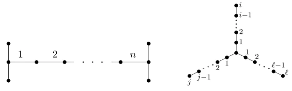
the class of forests of vertex degree at most 3 is a limit class for the the maximum independent setproblem. However, it is still not a minimal limit class, because by the same operation (double subdivisions of edges) one can destroy small induced copies of the graph Hn shown on the left of Figure 1. Therefore, the maximum
independent setproblem is NP-hard in the following class for each fixed value of k:
Zk is the class of (C3, . . . , Ck, H1, . . . , Hk)-free graphs of degree at most 3.
It is not difficult to see that the sequence Z3 ⊃ Z4 ⊃ . . . converges to the class of
forests every connected component of which has the form Si,j,ℓ represented on the
right of Figure 1, also known as tripods. Throughout the paper we denote this class by S, i.e.
S is the intersection of the sequence Z3 ⊃ Z4 ⊃ . . ..
The above discussion shows that S is a limit class for the maximum independent setproblem. Moreover, in [3] it was proved that S is a minimal limit class for this problem.
s s s ❵ ❵ ❵ s s s s s s 1 2 n s s s s s ❵ ❵ ❵ s s s s ❵ ❵ ❵ ✟ ✟ ✟ s s s s ❵ ❵ ❵ ❍❍ ❍ 1 2 i−1 i 1 2 j−1 j 1 2 ℓ−1 ℓ
Figure 1: Graphs Hn (left) and Si,j,ℓ (right).
Definition 3. A minimal (with respect to set inclusion) limit class for a problem Π is called a boundary class for Π.
The importance of the notion of boundary classes for NP-hard algorithmic graph prob-lems is due to the following theorem proved originally for the maximum independent set problem in [3] (can also be found in [4] in a more general context).
Theorem 4. If P 6= NP, then a finitely defined class X is Π-tough if and only if X contains a boundary class for Π.
In Section 4, we identify the first boundary class for the upper dominating set problem. To this end, we need a number of auxiliary results. The first of them is the following lemma dealing with limit classes, which was derived in [3, 4] as a step towards the proof of Theorem 4.
Lemma 4. If X is a finitely defined class containing a limit class for an NP-hard problem Π, then X is Π-tough.
The next two results were proved in [17] and [4], respectively.
Lemma 5. The minimum dominating set problem is NP-hard in the class Zk for each
fixed value of k.
Theorem 5. The class S is a boundary class for the minimum dominating set problem.
3
NP-hardness results
In this section, we prove two NP-hardness results about the upper dominating set problem in restricted graph classes.
3.1 Planar graphs of degree at most 6 and girth at least 6
Theorem 6. The upper dominating set problem restricted to the class of planar graphs with maximum vertex degree 6 and girth at least 6 is NP-hard.
Proof. We use a reduction from the maximum independent set problem (IS for short) in planar cubic graphs, where IS is NP-hard [13]. The input of the decision version of IS consists of a simple graph G = (V, E) and an integer k and asks to decide if G contains an independent set of size at least k.
Let G = (V, E) and an integer k be an instance of IS, where G is a planar cubic graph. We denote the number of vertices and edges of G by n and m, respectively. We build an instance G′ = (V′, E′) of the upper dominating set problem by replacing each edge e = uv ∈ E with two induced paths u − ve− ue− v and u − v′e− u′e− v, as shown in
Figure 2. t t t t t t t t ❅❅ ❅❅ u e v u v ve ue v′e u′e −→
Figure 2: Replacement of an edge by two paths
Clearly, G′ can be constructed in time polynomial in n. Moreover, it is not difficult to see that G′ is a planar graph with maximum vertex degree 6 and girth at least 6.
We claim that G contains an independent set of size at least k if and only if G′ contains a minimal dominating set of size at least k + 2m.
Suppose G contains an independent set S with |S| ≥ k and without loss of generality assume that S is maximal with respect to set-inclusion (otherwise, we greedily add vertices to S until it becomes a maximal independent set). Now we consider a set D ⊂ V′ containing
• all vertices of S,
• vertices ve and v′e for each edge e = uv ∈ E with v ∈ S,
• exactly one vertex in {ue, ve} (chosen arbitrarily) and exactly one vertex in {u′e, v′e}
(chosen arbitrarily) for each edge e = uv ∈ E with u, v 6∈ S.
It is not difficult to see that D is a maximal independent, and hence, by Lemma 2, a minimal dominating, set in G′. Moreover, |D| = |S| + 2m ≥ k + 2m.
To prove the inverse implication, we first observe the following:
• Every minimal dominating set in G′ contains either exactly two vertices or no vertex in the set {ue, ve, u′e, v′e} for every edge e = uv ∈ E. Indeed, assume a minimal
dominating set D in G′contains at least three vertices in {ue, ve, u′e, v′e}, say ue, ve, u′e.
But then D is not minimal, since uecan be removed from the set. If D contains one
vertex in {ue, ve, u′e, ve′}, say ue, then both u and v must belong to D (otherwise it
is not dominating), in which case it is not minimal (ue can be removed).
• If a minimal dominating set D in G′ contains exactly two vertices in {u
e, ve, u′e, v′e},
then
– one of them belongs to {ue, ve} and the other to {u′e, ve′}. Indeed, if both vertices
belong to {ue, ve}, then both u and v must also belong to D (to dominate u′e, ve′),
– at most one of u and v belongs to D. Indeed, if both of them belong to D, then Dis not minimal dominating, because u and v dominate the set {ue, ve, u′e, v′e}
and any vertex of this set can be removed from D.
Now let D ⊆ V′ be a minimal dominating set in G′ with |D| ≥ k + 2m. If D contains exactly two vertices in the set {ue, ve, u′e, v′e} for every edge e = uv ∈ E, then, according
to the discussion above, the set D ∩ V is independent in G and contains at least k vertices, as required.
Assume now that there are edges e = uv ∈ E for which the set {ue, ve, u′e, v′e} contains
no vertex of D. We call such edges D-clean. Obviously, both endpoints of a D-clean edge belong to D, since otherwise this set is not dominating. To prove the theorem in the situation when D-clean edges are present, we transform D into another minimal dominating set D′ with no D′-clean edges and with |D′| ≥ |D|. To this end, we do the
following. For each vertex u ∈ V incident to at least one D-clean edge, we first remove u from D, and then for each D-clean edge e = uv ∈ E incident to u, we introduce vertices ve, ve′ to D. Under this transformation vertex v may become redundant (i.e. its removal
may result in a dominating set), in which case we remove it. It is not difficult to see that the set D′ obtained in this way is a minimal dominating set with no D′-clean edges and with |D′| ≥ |D|. Therefore, D′∩ V is an independent set in G of cardinality at least k.
3.2 Complements of bipartite graphs
To prove one more NP-hardness result for the upper dominating set problem, let us introduce the following graph transformations. Given a graph G = (V, E), we denote by S(G) the incidence graph of G, i.e. the graph with vertex set V ∪ E, where V and E are
independent sets and a vertex v ∈ V is adjacent to a vertex e ∈ E in S(G) if and only if v is incident to e in G. Alternatively, S(G) is obtained from G by subdividing each edge e by a new vertex ve. According to this interpretation, we call E the set
of new vertices and V the set of old vertices. Any graph of the form S(G) for some Gwill be called a subdivision graph.
Q(G) the graph obtained from S(G) by creating a clique on the set of old vertices and a clique on the set of new vertices. We call any graph of the form Q(G) for some G a Q-graph.
The importance of Q-graphs for the upper dominating set problem is due to the following lemma, where we denote by Γ(G) the size of an upper dominating set in G and by γ(G) the size of a dominating set of minimum cardinality in G.
Lemma 6. Let G be a graph with n vertices such that Γ(Q(G)) ≥ 3. Then Γ(Q(G)) = n− γ(G).
Proof. Let D be a minimum dominating set in G, i.e. a dominating set of size γ(G). Without loss of generality, we will assume that D satisfies Lemma 3, i.e. every vertex of D has a private neighbour outside of D. For every vertex u outside of D, consider exactly one edge, chosen arbitrarily, connecting u to a vertex in D and denote this edge by eu. We claim that the set D′ = {veu : u 6∈ D} is a minimal dominating set in Q(G).
D, assume by contradiction that a vertex w ∈ D is not dominated by D′ in Q(G). By Lemma 3 we know that w has a private neighbour u outside of D. But then the edge e= uw is the only edge connecting u to a vertex in D. Therefore, ve necessarily belongs
to D′and hence it dominates w, contradicting our assumption. In order to show that D′ is a minimal dominating set, we observe that if we remove from D′a vertex v
euwith eu = uw,
u6∈ D, w ∈ D, then u becomes undominated in Q(G). Finally, since |D′| = n − |D|, we
conclude that Γ(Q(G)) ≥ n − |D| = n − γ(G).
Conversely, let D′ be an upper dominating set in Q(G), i.e. a minimal dominating set of size Γ(Q(G)) ≥ 3. Then D′ cannot intersect both V and E, since otherwise it contains exactly one vertex in each of these sets (else it is not minimal, because each of these sets is a clique), in which case |D′| = 2.
Assume first that D′ ⊆ V . Then V − D′ is an independent set in G. Indeed, if G contains an edge e connecting two vertices in V − D′, then vertex v
e is not dominated by
D′in Q(G), a contradiction. Moreover, V −D′ is a maximal (with respect to set-inclusion) independent set in G, because D′ is a minimal dominating set in Q(G). Therefore, V − D′ is a dominating set in G of size n − Γ(Q(G)) and hence γ(G) ≤ n − Γ(Q(G)).
Now assume D′ ⊆ E. Let us denote by G′ the subgraph of G formed by the edges
(and all their endpoints) e such that ve∈ D′. Then:
• G′ is a spanning forest of G, because D′ covers V (else D′ is not dominating in
Q(G)) and G′ is acyclic (else D′ is not a minimal dominating set in Q(G)).
• G′ is P4-free, i.e. each connected component of G′ is a star, since otherwise D′ is
not a minimal dominating set in Q(G), because any vertex of D′ corresponding to
the middle edge of a P4 in G′ can be removed from D′.
Let D be the set of the centers of the stars of G′. Then D is dominating in G (since
D′ covers V ) and |D| = n − |D′|, i.e. γ(G) ≤ n − Γ(Q(G)), as required.
Since the minimum dominating set problem is NP-hard and Q(G) is a co-bipartite graph, Lemma 6 leads to the following conclusion.
Theorem 7. The upper dominating set problem restricted to the class of complements of bipartite graphs is NP-hard.
4
A boundary class for upper domination
Since the upper dominating set problem is NP-hard in the class of complements of bipartite graphs, this class must contain a boundary class for the problem. An idea about the structure of such a boundary class comes from Theorem 5 and Lemma 6 and can be roughly described as follows: a boundary class for upper domination consists of graphs Q(G) obtained from graphs G in S. In order to transform this idea into a formal proof, we need more notations and more auxiliary results.
For an arbitrary class X of graphs, we denote S(X) := {S(G) : G ∈ X} and Q(X) := {Q(G) : G ∈ X}. In particular, Q(G) is the set of all Q-graphs, where G is the class of all simple graphs. We observe that an induced subgraph of a Q-graph is not necessarily a Q-graph. Indeed, in a Q-graph every new vertex is adjacent to exactly
two old vertices. However, by deleting some old vertices in a Q-graph we may obtain a graph in which a new vertex is adjacent to at most one old vertex. Therefore, Q(X) is not necessarily hereditary even if X is a hereditary class. We denote by Q∗(X) the hereditary closure of Q(X), i.e. the class obtained from Q(X) by adding to it all induced subgraphs of the graphs in Q(X). Similarly, we denote by S∗(X) the hereditary closure of S(X).
With the above notation, our goal is proving that Q∗(S) is a boundary class for the upper dominating setproblem. To achieve this goal we need the following lemmas. Lemma 7. Let X be a monotone class of graphs such that S 6⊆ X, then the clique-width of the graphs in Q∗(X) is bounded by a constant.
Proof. In [21], it was proved that if S 6⊆ X, then the clique-width is bounded for graphs in X. It is known (see e.g. [12]) that for monotone classes, the clique-width is bounded if and only if the tree-width is bounded. By subdividing the edges of all graphs in X exactly once, we transform X into the class S(X), where the tree-width is still bounded, since the subdivision of an edge of a graph does not change its tree-width. Since bounded tree-width implies bounded clique-width (see e.g. [12]), we conclude that S(X) is a class of graphs of bounded clique-width. Now, for each graph G in S(X) we create two cliques by complementing the edges within the sets of new and old vertices. This transforms S(X) into Q(X). It is known (see e.g. [16]) that local complementations applied finitely many times do not change the clique-width “too much”, i.e they transform a class of graphs of bounded clique-width into another class of graphs of bounded clique-width. Therefore, the clique-width of graphs in Q(X) is bounded. Finally, the clique-width of a graph is never smaller than the clique-width of any of its induced subgraphs (see e.g. [12]). Therefore, the clique-width of graphs in Q∗(X) is also bounded.
Lemma 8. Let X ⊆ Q∗(G) be a hereditary class. The clique-width of graphs in X is bounded by a constant if and only if it is bounded for Q-graphs in X.
Proof. The lemma is definitely true if X = Q∗(Y ) for some class Y . In this case, by definition, every non-Q-graph in X is an induced subgraph of a Q-graph from X. However, in general, X may contain a non-Q-graph H such that no Q-graph containing H as an induced subgraph belongs to X. In this case, we prove the result as follows.
First, we transform each graph H in X into a bipartite graph H′ by replacing the two
cliques of H (i.e. the sets of old and new vertices) with independent sets. In this way, X transforms into a class X′ which is a subclass of S∗(G). As we mentioned in the proof of Lemma 7, this transformation does not change the clique-width “too much”, i.e. the clique-width of graphs in X is bounded if and only if it is bounded for graphs in X′.
By definition, H ∈ X is a Q-graph if and only if H′ is a subdivision graph, i.e. H′ = S(G) for some graph G. Therefore, we need to show that the clique-width of graphs in X′ is bounded if and only if it is bounded for subdivision graphs in X′. In one
direction, the statement is trivial. To prove it in the other direction, assume the clique-width of subdivision graphs in X′ is bounded. If H′ is not a subdivision, it contains new vertices of degree 0 or 1. If H′ contains a vertex of degree 0, then it is disconnected, and
if H′ contains a vertex x of degree 1, then it has a cut-point (the neighbour of x). It is well-known that the clique-width of graphs in a hereditary class is bounded if and only if it is bounded for connected graphs in the class. Moreover, it was shown in [23] that the
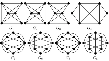
G1 G2 G3 G4
G5 G6 G7 G8
Figure 3: Forbidden graphs for Q∗(G)
clique-width of graphs in a hereditary class is bounded if and only if it is bounded for 2-connected graphs (i.e. 2-connected graphs without cut-points) in the class. Since 2-connected graphs without cut-points in X′ are subdivision graphs, we conclude that the clique-width
is bounded for all graphs in X′.
Finally, to prove the main result of this section, we need to show that Q∗(G) is a finitely
defined class. To show this, we first characterize graphs in Q∗(G) as follows: a graph G belongs to Q∗(G) if and only if the vertices of G can be partitioned into two (possibly empty) cliques U and W such that
(a) every vertex in W has at most two neighbours in U ,
(b) if x and y are two vertices of W each of which has exactly two neighbours in U , then N(x) ∩ U 6= N (y) ∩ U .
In the proof of the following lemma, we call any partition satisfying (a) and (b) nice. Therefore, Q∗(G) is precisely the class of graphs admitting a nice partition. Now we characterize Q∗(G) in terms of minimal forbidden induced subgraphs.
Lemma 9. Q∗(G) = Free(N ), where N is the set of eleven graphs consisting of C3, C5,
C7 and the eight graphs shown in Figure 3.
Proof. To show the inclusion Q∗(G) ⊆ Free(N ), we first observe that C
3, C5 and C7 are
forbidden in Q∗(G), since every graph in this class is co-bipartite, while C3, C5, C7 are
not co-bipartite. Each of the remaining eight graphs of the set N is co-bipartite, but none of them admits a nice partition, which is a routine matter to check.
To prove the inverse inclusion Free(N ) ⊆ Q∗(G), let us consider a graph G in Free(N ). By definition, G contains no C3, C5, C7. Also, since G1 is an induced subgraph of Ci
with i ≥ 9, we conclude that G contains no complements of odd cycles of length 9 or more. Therefore, G is co-bipartite. Let V1∪ V2 be an arbitrary bipartition of V (G) into
two cliques. In order to show that G belongs to Q∗(G), we split our analysis into several cases.
Case 1: G contains a K4 induced by vertices x1, y1 ∈ V1 and x2, y2 ∈ V2. To analyze
this case, we partition the vertices of V1 into four subsets with respect to x2, y2as follows:
A1 is the set of vertices of V1 adjacent to x2 and non-adjacent to y2,
B1 is the set of vertices of V1 adjacent to x2 and to y2,
C1 is the set of vertices of V1 adjacent to y2 and non-adjacent to x2,
D1 is the set of vertices of V1 adjacent neither to x2 nor to y2.
We partition the vertices of V2 with respect to x1, y1 into four subsets A2, B2, C2, D2
analogously. We now observe the following.
(1) For i ∈ {1, 2}, either Ai = ∅ or Ci = ∅, since otherwise a vertex in Ai and a vertex
in Ci together with x1, y1, x2, y2 induce G2.
According to this observation, in what follows, we may assume, without loss of generality, that
• C1 = ∅ and C2 = ∅.
We next observe that
(2) Either A1 = ∅ or A2 = ∅, since otherwise a vertex a1 ∈ A1 and a vertex a2 ∈ A2
together with x1, y1, x2, y2 induce either G1 (if a1 is not adjacent to a2) or G2 (if a1
is adjacent to a2).
Observation (2) allows us to assume, without loss of generality, that • A2 = ∅.
We further make the following conclusions:
(3) For i ∈ {1, 2}, |Di| ≤ 1, since otherwise any two vertices of Di together with
x1, x2, y1, y2 induce G3.
(4) If D1 = {d1} and D2 = {d2}, then d1 is adjacent to d2, since otherwise d1, d2, x1, x2,
y1, y2 induce G4.
(5) If A1 ∪ D1 ∪ D2 6= ∅, then every vertex of B1 is adjacent to every vertex of B2.
Indeed, assume, without loss of generality, that z ∈ A1∪ D1 and a vertex b1∈ B1 is
not adjacent to a vertex b2 ∈ B2. Then the vertices z, b1, b2, x1, x2, y1 induce either
G1 (if z is not adjacent to b2) or G2 (if z is adjacent to b2).
(6) Either A1= ∅ or D1= ∅, since otherwise a vertex in A1 and a vertex in D1 together
with x1, y1, x2, y2 induce G1.
According to (6), we split our analysis into three subcases as follows.
Case 1.1: D1 = {d1}. Then A1 = ∅ (by (6)) and every vertex of B1 is adjacent to
every vertex of B2 (by (5)). If D2 = ∅, then U = D1 and W = B1∪ B2 is a nice partition
Now assume D2 = {d2} and denote by B 0
1 the vertices of B1 nonadjacent to d2 and
by B1
1 the vertices of B1 adjacent to d2. Similarly, we denote by B 0
2 the vertices of B2
nonadjacent to d1 and by B21 the vertices of B2 adjacent to d1. Then |B11∪ B 1
2| ≤ 1, since
otherwise any two vertices of B1 1 ∪ B
1
2 together with x1, x2, d1, d2 induce G2. But then
U = D1∪ D2 and W = B1∪ B2 is a nice partition of G.
Case 1.2: A1 6= ∅. Then D1 = ∅ (by (6)) and every vertex of B1 is adjacent to every
vertex of B2 (by (5)). In this case, we claim that
(7) every vertex of B2 is either adjacent to every vertex of A1or to none of them. Indeed,
assume a vertex b2 ∈ B2 has a neighbour a′ ∈ A1 and a non-neighbour a′′ ∈ A1.
Then b2, a′, a′′, x1, y1, y2 induce G1.
We denote by B0
2 the subset of vertices of B2 that have no neighbours in A1 and by B 1 2
the subset of vertices of B2 adjacent to every vertex of A1. Then
• either |A1| = 1 or |B 0
2| = 1, since otherwise any two vertices of A1 together with any
two vertices of B0
2 and any two vertices of B1 induce G3.
• if D2 = {d2}, then |B21| = 1, since otherwise any two vertices of B 1
2 together with
d2, x1, y2 and any vertex a in A1 induce either G1 (if a is not adjacent to d2)) or G2
(if a is adjacent to d2)).
• if D2 = {d2}, then d2 has no neighbours in B1. Indeed, if d2has a neighbour b1 ∈ B1,
then vertices b1, d2, x1, x2, y2 together with any vertex a1 ∈ A1 induce either G1 (if
d2 is not adjacent to a1) or G2 (if d2 is adjacent to a1).
Therefore, either U = A1∪D2, W = B1∪B2(if |A1| = 1) or U = B 0 2∪D2, W = A1∪B1∪B 1 2 (if |B0 2| = 1) is a nice partition of G.
Case 1.3: A1 = ∅ and D1 = ∅. In this case, if D2 6= ∅, then U = D2, W = B1∪ B2
is a nice partition of G, since B1 ∪ B2 is a clique (by (5)). Assume now that D2 = ∅.
If B1∪ B2 is a clique, then G has a trivial nice partition. Suppose next that B1∪ B2 is
not a clique. If all non-edges of G are incident to a same vertex, say b (i.e. b is incident to all the edges of G), then U = {b}, W = (B1 ∪ B2) − {b} is a nice partition of G.
Otherwise, G contains a pair of non-edges b′
1b′2 6∈ E(G) and b′′1b′′2 6∈ E(G) with all four
vertices b′1, b′′1 ∈ B1, b′2, b′′2 ∈ B2 being distinct (i.e. b′1b′2 and b′′1b′′2 form a matching in
G). We observe that {b′1, b′′1, b′2, b′′2} ∩ {x1, y1, x2, y2} = ∅, because by definition vertices
x1, y1, x2, y2 dominate the set B1∪ B2. But then b′1, b′′1, b′2, b′′2, x1, y1 induce either G2 (if
both b′1b′′2 and b′2b′′1 are edges in G) or G1 (if exactly one of b′1b′′2 and b′2b′′1 is an edge in G)
or G3 (if neither b′1b′′2 nor b′2b′′1 is an edge in G). This completes the proof of Case 1.
Case 2: G contains no K4 with two vertices in V1 and two vertices in V2. We claim
that in this case V1∪ V2 is a nice partition of G. First, the assumption of case 2 implies
that that no two vertices in the same part of the bipartition V1 ∪ V2 have two common
neighbours in the opposite part, verifying condition (b) of the definition of nice partition. To verify condition (a), it remains to prove that one of the parts V1 and V2 has no vertices
with more than two neighbours in the opposite part. Assume the contrary and let a1∈ V1
First, suppose a1 is adjacent to a2. Denote by b2, c2 two other neighbours of a1 in V2
and by b1, c1 two other neighbours of a2in V1. Then there are no edges between b1, c1 and
b2, c2, since otherwise we are in conditions of Case 1. But now a1, b1, c1, a2, b2, c2 induce a
G3.
Suppose now that a1 is not adjacent to a2. We denote by b2, c2, d2 three neighbours of
a1 in V2 and by b1, c1, d1 three neighbours of a2 in V1. No two edges between b1, c1, d1 and
b2, c2, d2 (if any) share a vertex, since otherwise we are in conditions of Case 1. But then
a1, b1, c1, d1, a2, b2, c2, d2induce either G5 or G6 or G7 or G8. This contradiction completes
the proof of the lemma.
Now we are ready to prove the main result of the section.
Theorem 8. If P 6= NP, then Q∗(S) is a boundary class for the upper dominating set problem.
Proof. From Lemmas 5 and 6 we know that upper domination is NP-hard in the class Q∗(Zk) for all values of k ≥ 3. Also, it is not hard to verify that the sequence of classes
Q∗(Z1), Q∗(Z2) . . . converges to Q∗(S). Therefore, Q∗(S) is a limit class for the upper
dominating set problem. To prove its minimality, assume there is a limit class X which is properly contained in Q∗(S). We consider a graph F ∈ Q∗(S) − X, a graph
G ∈ Q(S) containing F as an induced subgraph (possibly G = F if F ∈ Q(S)) and a graph H ∈ S such that G = Q(H). From the choice of G and Lemma 9, we know that X ⊆ Free(N ∪ {G}), where N is the set of minimal forbidden induced subgraphs for the class Q∗(G). Since the set N is finite (by Lemma 9), we conclude with the help of Lemma 4 that the upper dominating set problem is NP-hard in the class Free(N ∪{G}). To obtain a contradiction, we will show that graphs in Free(N ∪ {G}) have bounded clique-width.
Denote by M the set of all graphs containing H as a spanning subgraph. Clearly Free(M ) is a monotone class. More precisely, it is the class of graphs containing no H as a subgraph (not necessarily induced). Since Free(M ) is monotone and S 6⊂ Free(M) (as H∈ S), we know from Lemma 7 that the clique-width is bounded in Q∗(Free(M )).
To prove that graphs in Free(N ∪ {G}) have bounded clique-width, we will show that Q-graphs in this class belong to Q∗(Free(M )). Let Q(H′) be a Q-graph in Free(N ∪ {G}).
Since the vertices of Q(H′) represent the vertices and the edges of H′ and Q(H′) does not contain G as an induced subgraph, we conclude that H′ does not contain H as a subgraph. Therefore, H′ ∈ Free(M ), and hence Q(H′) ∈ Q(Free(M )). By Lemma 8, this
implies that all graphs in Free(N ∪ {G}) have bounded clique-width. This contradicts the fact that the upper dominating set problem is NP-hard in this class and completes the proof of the theorem.
5
A dichotomy in monogenic classes
The main goal of this section is to show that in the family of monogenic classes the upper dominating setproblem admits a dichotomy, i.e. for each graph H, the problem is either polynomial-time solvable or NP-hard for H-free graphs. We start with polynomial-time results.
5.1 Polynomial-time results
As we have mentioned in the introduction, the upper dominating set problem can be solved in polynomial time for bipartite graphs [10], chordal graphs [15] and generalized series-parallel graphs [14]. It also admits a polynomial-time solution in any class of graphs of bounded clique-width [11]. Since P4-free graphs have clique-width at most 2 (see e.g.
[8]), we make the following conclusion.
Proposition 1. The upper dominating set problem can be solved for P4-free graphs in
polynomial time.
In what follows, we develop a polynomial-time algorithm to solve the problem in the class of 2K2-free graphs.
We start by observing that the class of 2K2-free graphs admits a polynomial-time
solution to the maximum independent set problem (see e.g. [25]). By Lemma 2 every maximal (and hence maximum) independent set is a minimal dominating set. These observations allow us to restrict ourselves to the analysis of minimal dominating sets X such that
• X contains at least one edge, • |X| > α(G),
where α(G) is the independence number, i.e. the size of a maximum independent set in G.
Let G be a 2K2-free graph and let ab be an edge in G. Assuming that G contains a
minimal dominating set X containing both a and b, we first explore some properties of X. In our analysis we use the following notation. We denote by
• N the neighbourhood of {a, b}, i.e. the set of vertices outside of {a, b} each of which is adjacent to at least one vertex of {a, b},
• A the anti-neighbourhood of {a, b}, i.e. the set of vertices adjacent neither to a nor to b,
• Y := X ∩ N ,
• Z := N (Y ) ∩ A, i.e. the set of vertices of A each of which is adjacent to at least one vertex of Y .
Since a and b are adjacent, by Lemma 2 each of them has a private neighbour outside of X. We denote by
• a∗ a private neighbour of a,
• b∗ a private neighbour of b.
By definition, a∗and b∗belong to N −Y and have no neighbours in Y . Since G is 2K2-free,
we conclude that
Claim 1. A is an independent set.
We also derive a number of other helpful claims. Claim 2. Z ∩ X = ∅ and A − Z ⊆ X.
Proof. Assume a vertex z ∈ Z belongs to X. Then X − {z} is a dominating set, because z does not dominate any vertex of A (since A is independent) and it is dominated by its neighbor in Y . This contradicts the minimality of X and proves that Z ∩ X = ∅. Also, by definition, no vertex of A − Z has a neighbour in Y ∪ {a, b}. Therefore, to be dominated A− Z must be included in X.
Claim 3. If |X| > α(G), then |Y | = |Z| and every vertex of Z is a private neighbor of a vertex in Y .
Proof. Since every vertex y in Y belongs to X and has a neighbour in X (a or b), by Lemma 2 y must have a private neighbor in Z. Therefore, |Z| ≥ |Y |. If |Z| is strictly greater than |Y |, then |X| ≤ |A ∪ {a}| ≤ α(G) (since A is independent), which contradicts the assumption |X| > α(G). Therefore, |Y | = |Z| and every vertex of Z is a private neighbor of a vertex in Y .
Claim 4. If |Y | > 1 and |X| > α(G), then Y ⊆ N (a) ∩ N (b).
Proof. Let y1, y2 be two vertices in Y and let z1, z2 be two vertices in Z which are private
neighbours of y1 and y2, respectively.
Assume a is not adjacent to y1, then b is adjacent to y1 (by definition of Y ) and a∗
is adjacent to z1, since otherwise the vertices a, a∗, y1, z1 induce a 2K2 in G. Also, a∗ is
adjacent to z2, since otherwise a 2K2 is induced by a∗, z1, y2, z2. But now the vertices
a∗, z2, b, y1 induce a 2K2. This contradiction shows that a is adjacent to y1. Since y1 has
been chosen arbitrarily, a is adjacent to every vertex of Y , and by symmetry, b is adjacent to every vertex of Y .
Claim 5. If |Y | > 1 and |X| > α(G), then a∗ and b∗ have no neighbours in Z.
Proof. Assume by contradiction that a∗ is adjacent to a vertex z1 ∈ Z. By Claim 3, z1 is
a private neighbour of a vertex y1 ∈ Y . Since |Y | > 1, there exists another vertex y2 ∈ Y
with a private neighbor z2∈ Z. From Claim 4, we know that b is adjacent to y2. But then
the set {b, y2, a∗, z1} induces a 2K2. This contradiction shows that a∗ has no neighbours
in Z. By symmetry, b∗ has no neighbours in in Z.
The above series of claims leads to the following conclusion, which plays a key role for the development of a polynomial-time algorithm.
Lemma 10. If |X| > α(G), then |Y | = 1 and Y ⊆ N (a) ∩ N (b).
Proof. First, we show that |Y | ≤ 1. Assume to the contrary that |Y | > 1. By definition of a∗ and Claim 2, vertex a∗has no neighbours in A−Z, and by Claim 5, a∗has no neighbours in Z. Therefore, A ∪ {a∗, b} is an independent set of size |X| = |Y | + |A − Z| + 2. This contradicts the assumption that |X| > α(G) and proves that |Y | ≤ 1.
Suppose now that |Y | = 0. Then, by Claim 3, |Z| = 0 and hence, by Claim 2, X = A ∪ {a, b}. Also, by definition of a∗, vertex a∗ has no neighbours in A. But then A∪ {a∗, b} is an independent set of size |X|, contradicting that |X| > α(G).
From the above discussion we know that Y consists of a single vertex, say y. It remains to show that y is adjacent to both a and b. By definition, y must be adjacent to at least
one of them, say to a. Assume that y is not adjacent to b. By definition of a∗, vertex a∗ has no neighbours in {y} ∪ (A − Z), and by definition of Z, vertex y has no neighbours in A− Z. But then (A − Z) ∪ {a∗, b, y} is an independent set of size |X| = |Y | + |A − Z| + 2.
This contradicts the assumption that |X| > α(G) and shows that y is adjacent to both a and b.
Corollary 1. If a minimal dominating set in a 2K2-free graph G is larger than α(G),
then it consists of a triangle and all the vertices not dominated by the triangle.
In what follows, we describe an algorithm A to find a minimal dominating set M with maximum cardinality in a 2K2-free graph G in polynomial time. In the description of
the algorithm, given a graph G = (V, E) and a subset U ⊆ V , we denote by A(U ) the anti-neighbourhood of U , i.e. the subset of vertices of G outside of U none of which has a neighbour in U .
Algorithm A
Input: A 2K2-free graph G = (V, E).
Output: A minimal dominating set M in G with maximum cardinality. 1. Find a maximum independent set M in G.
2. For each triangle T in G: • Let M′:= T ∪ A(T ).
• If M′ is a minimal dominating set and |M′| > |M |, then M := M′. 3. Return M .
Theorem 9. Algorithm A correctly solves the upper dominating set problem for 2K2
-free graphs in polynomial time.
Proof. Let G be a 2K2-free graph with n vertices. In O(n2) time, one can find a maximum
independent set M in G (see e.g. [25]). Since M is also a minimal dominating set (see Lemma 1), any solution of size at most α(G) can be ignored.
If X is a solution of size more than α(G), then, by Corollary 1, it consists of a triangle T and its anti-neighbourhood A(T ). For each triangle T , verifying whether T ∪ A(T ) is a minimal dominating set can be done in O(n2
) time. Therefore, the overall time complexity of the algorithm can be estimated as O(n5
).
5.2 The dichotomy
In this section, we summarize the results presented earlier in order to obtain the following dichotomy.
Theorem 10. Let H be a graph. If H is a 2K2 or P4 (or any induced subgraph of 2K2
or P4), then the upper dominating set problem can be solved for H-free graphs in
polynomial time. Otherwise the problem is NP-hard for H-free graphs.
• either by Theorem 6 if k ≤ 5, because in this case the class of H-free graphs contains all graphs of girth at least 6,
• or by Theorem 7 if k ≥ 6, because in this case the class of H-free graphs contains the class of K3-free graphs and hence all complements of bipartite graphs.
Assume now that H is acyclic, i.e. a forest. If it contains a claw (a star whose center has degree 3), then the problem is NP-hard for H-free graphs by Theorem 7, because in this case the class of H-free graphs contains all K3-free graphs and hence all complements of
bipartite graphs.
If H is a claw-free forest, then every connected component of H is a path. If H contains at least three connected components, then the class of H-free graphs contains all K3-free
graphs, in which case the problem is NP-hard by Theorem 7. Assume H consists of two connected components Pk and Pt.
• If k + t ≥ 5, then the class of H-free graphs contains all K3-free graphs and hence
the problem is NP-hard by Theorem 7.
• If k + t ≤ 3, then the class of H-free graphs is a subclass of P4-free graphs and hence
the problem can be solved in polynomial time in this class by Proposition 1. • If k + t = 4, then
– either k = t = 2, in which case H = 2K2 and hence the problem can be solved
in polynomial time by Theorem 9,
– or k = 4 and t = 0, in which case H = P4 and hence the problem can be solved
in polynomial time by Proposition 1,
– or k = 3 and t = 1, in which case the class of H-free graphs contains all K3-free
graphs and hence the problem is NP-hard by Theorem 7.
6
Conclusion
In this paper, we identified the first boundary class for the upper dominating set problem and proved that the problem admits a dichotomy for monogenic classes, i.e. classes defined by a single forbidden induced subgraph. We conjecture that this dichotomy can be extended to all finitely defined classes. By Theorem 4, the problem is NP-hard in a finitely defined class X if and only if X contains a boundary class for the problem. In the present paper, we made the first step towards the description of the family of boundary classes for upper domination. Since the problem is NP-hard in the class of triangle-free graphs (Theorem 6), there must exist at least one more boundary class for the problem. We believe that this is again the class S of tripods. This class was proved to be boundary for many algorithmic graph problems, which is typically done by showing that a problem is NP-hard in the class Zk for any fixed value of k. We believe that the same is true for
upper domination, but this question remains open.
One more open question deals with Lemma 6 of the present paper. It shows a rela-tionship between minimum dominating set in general graphs and upper dominating
set in co-bipartite graphs. For the first of these problems, three boundary classes are available [4]. One of them was transformed in the present paper to a boundary class for upper domination. Whether the other two can also be transformed in a similar way is an interesting open question, which we leave for future research.
Acknowledgements
Vadim Lozin and Viktor Zamaraev gratefully acknowledge support from EPSRC, grant EP/L020408/1.
Part of this research was carried out when Vadim Lozin was visiting the King Abdullah University of Science and Technology (KAUST). This author thanks the University for hospitality and stimulating research environment.
References
[1] H. AbouEisha, S. Hussain, V. Lozin, J. Monnot, B. Ries, A dichotomy for upper domination in monogenic classes, Lecture Notes in Computer Science, 8881, 258–267 (2014)
[2] H. AbouEisha, S. Hussain, V. Lozin, J. Monnot, B. Ries, V. Zamaraev, A boundary property for upper domination, Lecture Notes in Computer Science, 9843, 229–240 (2016)
[3] V.E. Alekseev, On easy and hard hereditary classes of graphs with respect to the independent set problem, Discrete Applied Mathematics, 132, 17–26 (2003)
[4] V.E. Alekseev, D.V. Korobitsyn, V.V. Lozin, Boundary classes of graphs for the dominating set problem, Discrete Mathematics. 285, 1–6 (2004)
[5] V.E. Alekseev, R. Boliac, D.V. Korobitsyn, V.V. Lozin, NP-hard graph problems and boundary classes of graphs, Theoretical Computer Science. 389, 219–236 (2007) [6] C. Bazgan, L. Brankovic, K. Casel, H. Fernau, K. Jansen, K.-M. Klein, M. Lampis,
M. Liedloff, J. Monnot, V.Th. Paschos, Algorithmic Aspects of Upper Domination: A Parameterised Perspective, Lecture Notes in Computer Science, 9778, 113–124 (2016) [7] C. Bazgan, L. Brankovic, K. Casel, H. Fernau, K. Jansen, K.-M. Klein, M. Lampis, M. Liedloff, J. Monnot, V.Th. Paschos, Upper Domination: Complexity and Approx-imation, Lecture Notes in Computer Science, 9843, 241–252 (2016)
[8] A. Brandst¨adt, J. Engelfriet, H.-O. Le, V.V. Lozin, Clique-width for 4-vertex forbid-den subgraphs, Theory of Computing Systems 39(4), 561–590 (2006)
[9] G.A. Cheston, G. Fricke, S.T. Hedetniemi, D.P. Jacobs, On the computational com-plexity of upper fractional domination, Discrete Applied Mathematics. 27(3), 195–207 (1990)
[10] E.J. Cockayne, O. Favaron, C. Payan, A.G. Thomason, Contributions to the theory of domination, independence and irredundance in graphs, Discrete Mathematics. 33(3), 249–258 (1981)
[11] B. Courcelle, J.A. Makowsky, U. Rotics, Linear time solvable optimization problems on graphs of bounded clique-width, Theory of Computing Systems. 33(2), 125–150 (2000)
[12] B. Courcelle, S. Olariu, Upper bounds to the clique-width of a graph, Discrete Applied Mathematics. 101, 77-114 (2000)
[13] M.R. Garey, D.S. Johnson, L.J. Stockmeyer, Some Simplified NP-Complete Graph Problems, Theoretical Computer Science. 1(3), 237–267 (1976)
[14] E.O. Hare, S.T. Hedetniemi, R.C. Laskar, K. Peters, T. Wimer, Linear-time com-putability of combinatorial problems on generalized-series-parallel graphs, In D. S. Johnson et al., editors, Discrete Algorithms and Complexity (Academic Press, New York), 437–457, 1987.
[15] M.S. Jacobson, K. Peters, Chordal graphs and upper irredundance, upper domination and independence, Discrete Mathematics. 86(1-3), 59–69 (1990)
[16] M. Kami´nski, V. Lozin, M. Milaniˇc, Recent developments on graphs of bounded clique-width, Discrete Applied Mathematics. 157, 2747–2761 (2009)
[17] D.V. Korobitsyn, On the complexity of determining the domination number in mono-genic classes of graphs, Diskretnaya Matematika. 2(3), 90–96 (1990) (in Russian, translation in Discrete Math. Appl. 2 (1992), no. 2, 191-199).
[18] N. Korpelainen, V.V. Lozin, D.S. Malyshev, A. Tiskin, Boundary Properties of Graphs for Algorithmic Graph Problems, Theoretical Computer Science. 412, 3545– 3554 (2011)
[19] N. Korpelainen, V. Lozin, I. Razgon, Boundary properties of well-quasi-ordered sets of graphs, Order. 30, 723-735 (2013)
[20] V.V. Lozin, Boundary classes of planar graphs, Combinatorics, Probability and Com-puting. 17, 287–295 (2008)
[21] V. Lozin, M. Milaniˇc, Critical properties of graphs of bounded clique-width, Discrete Mathematics. 313, 1035-1044 (2013)
[22] V. Lozin, C. Purcell, Boundary properties of the satisfiability problems, Information Processing Letters. 113, 313-317 (2013)
[23] V. Lozin, D. Rautenbach, On the band-, tree- and clique-width of graphs with bounded vertex degree, SIAM J. Discrete Mathematics. 18, 195-206 (2004)
[24] V. Lozin, V. Zamaraev, Boundary properties of factorial classes of graphs, J. Graph Theory. 78, 207–218 (2015)
[25] V.V. Lozin, R. Mosca, Independent sets in extensions of 2K2-free graphs, Discrete
Applied Mathematics. 146(1), 74–80 (2005)
[26] O.J. Murphy, Computing independent sets in graphs with large girth, Discrete Applied Mathematics. 35, 167–170 (1992)
[27] N. Robertson, P.D. Seymour, Graph minors. V. Excluding a planar graph. J. Combin. Theory Ser. B. 41, no. 1, 92–114 (1986)