Modelling a manufacturing line using extended object oriented bayesian network

Open Archive Toulouse Archive Ouverte (OATAO)

OATAO is an open access repository that collects the work of some Toulouse

researchers and makes it freely available over the web where possible.

This is

version published in:

Official URL :

https://doi.org/10.1016/j.ifacol.2017.08.1011

To cite this version :

Any correspondence concerning this service should be sent to the repository administrator: [email protected]

Liu, Quan and Tchangani, Ayeley and Pérès, François Modelling a manufacturing line

using extended object oriented bayesian network. (2017) IFAC-PapersOnLine, 50 (1).

6196-6201. ISSN 2405-8963

OATAO

10.1016/j.ifacol.2017.08.1011

Modelling a Manufacturing Line usi g

Extended Object Oriented Bayesian

Network

y

E

d O j

O

d B y

Extended Ob ect Or e ted Bay ia

N t o

∗_{Universit´e F´ed´erale Toulouse Midi-Pyr´en´ees - Laboratoire G´enie de}

Production, INP-ENIT, 65016 France (e-mail: quan.liu@ enit.fr).

∗∗_{Universit´e F´ed´erale Toulouse Midi-Pyr´en´ees - Laboratoire G´enie de}

Production, INP-ENIT, 65016 France (e-mail: ayeley.tchangani@ iut-tarbes.fr).

∗∗∗_{Universit´e F´ed´erale Toulouse Midi-Pyr´en´ees - Laboratoire G´enie de}

Production, INP-ENIT, 65016 France (e-mail: francois.peres@ enit.fr).

Extended Object Oriented Bay sian

Network

U e Fede l To l d e e Ge d

Pr ducti I P E IT 65016 Franc e mail quan li @ en t fr)

Univers te Federale To l use Mid P renees Lab rat ire e ie de

Pr duct I P E IT 5016 Fra ce e mail a eley tchangani@

iut tarbes r

Uni e si e Fede ale To l use M d P e ees La a i e Ge ie de

Pr d ct n I P E IT 65016 Fran e e mail ra c is peres@ enit r)

Abstract: Bayesian Network (BN) is a widely used modelling tool in probabilistic reasoning; however it turns out to be difficult to use this tool to model a large scale complex system such as a manufacturing line due to the number of parameters when the system exceeds a certain amount of components. Motivated by the necessity to both reduce the complexity of the model while increasing the capacity of integrating a large number of parameters, this communication ambitions to propose a new modelling approach, called Extended Object Oriented Bayesian Network (EOOBN). The EOOBN is an underlying mathematical tool which has much more flexibility than classical Bayesian Networks. The main aim of the communication is then to present a methodology dedicated to EOOBN construction. After having introduced the main concepts and described the EOOBN building principles, an industrial application is proposed to illustrate the developments.

M d lli

M

i

Li

i

E

d d

j

i

d B y i

N

k

Q. Liu∗ _{A. Tchangani}∗∗ _F.P´er`es∗∗∗

U s ´ F´ed´e le To louse Mid y ´e ´ a ir G´e i d

io I P E IT, 6 F ce (e il q li ni f )

U i si ´ F´ed´e le To lo e Mi i y ´e ´ L oi ´ ie

i I E IT 6 F c ( il l i

i bes )

U i e it´ F´d´e le Toul u e Midi y ´ ´ La i ´ni

i I E IT F ( il i p

i )

Abstract Bayesian N twork (BN i a wide y us d model ng too in p obabilis c reasoning

how ver it turns ou to be d fficult o use th ool to mod a la ge sca e complex y t m such

as a manu acturing lin due to the number o parameters when he y tem exc ed a ertain amount of c mpone ts Moti ated by the nec ssi y to both reduce the complex ty of the model

while incr as ng the c pacity of integra ing a larg numb r of parameters, is communication

ambition to propo a new mode ing pproach, called Extended Ob ect O ient d Ba esian

Netw rk EOO N) Th EOOB is an un rlying ma hemat cal ool which has uch m re

flexibili y than classic Bayesian N tw rks The main aim o the communication s then to

p esent a me hodology ded cated to EOOBN cons ructi n. Af er having in roduc d the main concepts and desc ibed the E

Keywords: complex system, modelling, Extended Object Oriented Bayesian Network, risk management

1. INTRODUCTION

Due to dynamic evolution of industrial production systems and the multiplicity of interactions among its constitutive elements, an abnormality or a component failure may result in a cascade phenomenon that can lead to unaccept-able risks or to the collapse of such networked systems. Within this framework an efficient tool is required to assist decision-makers. The modelling tool should simulate the system’s behaviour by considering all together the character dynamic and uncertain associated with the big amount of variables related to complex systems. Supplying such a decision support system becomes a challenge for researchers. Modelling risks requires indeed considering the nature of the relationships (influence, causality, etc.), the related uncertainties (about the existence of a rela-tionship, of its intensity or even about the delimitation of the system under consideration), the evolution dynamic (modification over the time of the model structure and/or parameters) Kamissoko et al. (2011), Godichaud et al. (2012a),Bouzarour-Amokrane et al. (2015). Taking into account of all these characteristics, is likely to result to a complex and large scale system P´er`es and Grenouilleau (2002),Godichaud et al. (2011). In this communication, we attempt to model such a system through an exten-sion of Bayesian Network techniques subsequently referred as Extended Object Bayesian networks (EOOBN) based

on components sharing a same structure. The main idea is first to use Bayesian networks properties to describe elementary components characterized by uncertainties of interactions among their constitutive variables. Then the whole system will be described by associating these compo-nents through object oriented mechanisms. This modelling approach will help monitoring and measuring the evolution of the system for a better understanding and control-ling of its behaviour. The communication is structured as follows. Section 2 gives a brief overview of complex systems and Bayesian Networks. Section 3 presents the Extended Object Oriented Bayesian Networks (EOOBN) and its application in modelling a manufacturing line. Simulation results are provided. Finally, a conclusion and some perspectives are presented in the last section.

2. COMPLEX SYSTEMS AND BAYESIAN NETWORKS

2.1 Complex systems

A complex system is composed of a large number of components. These components are often interconnected through uncertain and dynamic relationships. The goal of this communication is to propose a new modelling approach for the characterization of these complex sys-tems in order to evaluate the resulting performance when one or several components are either destabilized by an

ff ff ff ff ff ff

external event or affected by an internal issue. Such kind of model can be used to assess some key indicators and assist the decision making process. It can be applied to different domains such as economy, medicine, production and many other fields. In Amaral and Ottino (2004), the author points out issues related to classical modelling methods based on assumptions which eventually can skew the results by ignoring the aspects of interdependency, dynamic and size of the system. Finding another ap-proach to simulate these complex systems when avoiding a great number of hypothesis is worth of research. Bayesian Networks are very efficient for modelling uncertainties. Meanwhile Dynamic Bayesian Network may be used when there is a temporal dimension in the system behaviour Murphy (2002). In the case of system with a huge number of components, a possibility to reduce this complexity is to use the so called Object Oriented Bayesian Networks (OOBN) in order to exploit possibilities offered by this modelling technique. The idea of modelling repeatable systems by object oriented techniques has been already considered in a certain number of studies such as Jaeger (2000),Weber and Jouffe (2006) to mention just a few. In the following paragraph, we introduce basics of static and dynamic Bayesian network characteristics.

2.2 Bayesian Networks

A Bayesian Network is a directed acyclic graph (DAG) that represents a certain relationships (in general causal relationships) between variables in a certain knowledge domain; each node represents a random variable associated with a conditional probability table (CPT) characterizing its parameters. Bayes theorem is the central theory in the mechanism of inference in Bayesian Networks. It permits to propagate some local observations through the graph in order to update a priori knowledge about the state of other nodes Nielsen and Jensen (2009), Pearl (1988). Figure 1 shows an example of a Bayesian Network which has three nodes A, B and C. The nodes A and B are the parents of C. There are two types of probability tables in a BN Godichaud et al. (2012b): prior probabilities tables for root variables (variables without parents) like A and B and conditional probabilities tables for variables with parents like C Godichaud et al. (2012a),Godichaud et al. (2012b). Indeed, a BN model is not only a static representation of knowledge but also a tool for the evidence inference which updates the probabilities in the network and enables the refinement of the results according to the observed situation Ben Hassen et al. (2013).

Fig. 1. Bayesian Network

Dynamic Bayesian Network In order to take into

ac-count of possible dynamic behaviour of systems, dynamic

Bayesian networks (DBN), are introduced as a possible extension of a BN. The DBN is a series of time-slice BN corresponding to a Hidden Markov Model (HMM) Rabiner and Juang (1986),Murphy (2002). In the former example of Fig.1, if we assume that B evolves over time, so that the node B becomes a dynamic node then Fig.2 shows the corresponding DBN model with 2 time-slices, where the

dynamic node is Bti. The communication between

time-slices uses the transition model determined by a transition matrix A as:

• the transition model: A = P (Bti|Bti−1)

• the intial state: π = P (Bt0)

Fig. 2. Dynamic Bayesian Network with two time slices

Object Oriented Bayesian Network Using BN techniques

for modelling risk assessment processes becomes all the time more complex when the size of the system increases. For a large scale system with many interacting elements, constructing a BN to represent its functioning behaviour may be very challenging. Meanwhile, when the size of network grows, the model visibility reduces and the update of parameter becomes burdensome. For this reason, an object oriented techniques might be an alternative to reduce the complexity by highlighting a generic pattern representative of the various dimensions of the problem. An object oriented Bayesian network (OOBN), is a direct application of the object paradigm Bangsø and Wuillemin (2000), Koller and Pfeffer (1997). The basic element is the class, fragment of a Bayesian network who has three sets of nodes: input, output and internal nodes see Figure 3. The input and output nodes are the interface of a class which can be seen from the outside.

Fig. 3. Object Oriented Bayesian Network

The OOBN takes advantage of classic BN but introduces the concept of instance nodes. An instance node is an abstraction of a part of a network which can be used as an elementary component to represent the whole structure. The notion of encapsulation allows the transmission of all properties of the network fragment. An object oriented network can be viewed as a hierarchical description/model of a problem. This makes the modelling process easier since the OOBN-fragments at different levels of abstraction are more readable. An OOBN model can be built through expertise or by using learning techniques. In Langseth and Nielsen (2003) and Wuillemin and Torti (2012), the

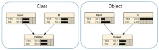
Tra11sitio11model: P(Be,IBi,_,)

Class Object

...

...

/

authors give some insights into OOBN structure learn-ing. The construction of such a model can be facilitated by ontology representation Liu et al. (2015). Once the structure of the system is defined, the Conditional Prob-ability Tables (CPTs, also called parameters) have to be parametrized. In Langseth and Bangsø (2001) the author extend the parameter learning algorithm to the objects who have the same structure based on OO assumption. The parameters being identical, this reduces the number of parameters to be specified or learnt. Modelling a complex system by an OOBN allows reducing the design work. However, most of existing works dealing with this topic consider that parameters do not change from an object to another which may not be a realistic assumption in a real world problem modelling context. As our main goal is to use OOBN for the representation of a large, repeatable and inherited system, this shortcoming must be remedied. In the next part, we will introduce an Extended Object Oriented Bayesian Network or EOOBN Liu et al. (2016).

3. EXTENDED OBJECT ORIENTED BAYESIAN NETWORKS

The Extended Object Oriented Bayesian Network was first introduced in Liu et al. (2016). Because decision-makers require both flexibility in parameter variation as well as the capacity of their tools to consider dynamic evolution, we propose here to deal with a methodology making easier the construction work of a model characterizing a large repeatable system.

The construction of EOOBN begins by defining the struc-ture through the notion of class, as specified below. Class: A class (C) is the structure part (S) in a BN independently of the CPT parameter values. It has three kinds of nodes namely: input nodes, output nodes and internal nodes. Only the input and output nodes are visible from outside the class.

The instantiation (specifying modalities and parameters of nodes defined in the class) of classes give rise to the object.

Object: An object (O{S, P }) in an OOBN is an

instan-tiation of the corresponding class. There are two parts in an object, the structure (S) which inherits from the class and the parameters (P ) which will be defined by experts or learning processes.

Distinguishing class and object permits the parameter variation, in the sense that objects will not have the same parameters as it is usually assumed in the literature. Al-though in Bangsø and Wuillemin (2000) a DBN simulation approach is given based on a self-reference node in an object, a confusion might appear when trying to add the dynamic part within a large OOBN. To overcome this issue, we introduce the virtual nodes in the EOOBN to simulate the dynamic part. We then obtain a dynamic EOOBN which herein after referred to as a DOOBN. We call input and output nodes as communication channel for the class/object entity because they are in charge of exchanging information for the class/object. Here are some conditions that must be satisfied Liu et al. (2016):

• Input nodes cannot have parents inside the class

• An input node is a reference node which is the projection of an output or a normal upstream node • Internal nodes cannot have neither parents nor

chil-dren outside the class

• Output nodes cannot have child inside the class These conditions help the designer to build the class/object more easily and make the model much more understand-able. At the same time each object remains independent which will turn out to be helpful when developing the relative inference techniques.

With the purpose of introducing the dynamic evolution into the EOOBN, we propose the concept of virtual node enabling the communication between time-slices.

Virtual node: The virtual node is a communication channel for the class/object. It usually stands for the dynamic node.

• The virtual node is either an input node or an output node in the class/object

• It is added for dynamic node in the class/object as a communication channel with other time-slices • The transition model represents the parameters

be-tween the virtual input and the dynamic node. Con-ditional probabilities between a dynamic node and its virtual output are equalled to 1

The virtual node encapsulates the dynamic evolution infor-mation into the class/object which keeps the independency between the objects. In the meantime, using the virtual node helps us to build the dynamic development clearly.

Construction method

The construction of a dynamic EOOBN can be done by carrying out the following steps:

(1) Formalize the structure S of a system (by splitting the system into different classes C)

(2) Design the structure of each class (C) with respect to S and without considering the dynamic part

(3) Identify the dynamic nodes in the class Nti and add

the virtual input and output nodes around these dynamic nodes

(4) Instantiate the classes by introducing the parameters corresponding to the object

(5) Connect the objects through their communication channels

From the construction method, we first build the model without considering the dynamic evolution because of the virtual nodes. By using the virtual nodes, the designer could treat the dynamic evolution as an independent part in the system. The modification of the model is then much more flexible since the designer has the possibility to add the dynamic information at any time. Virtual nodes can not only help us building a dynamic model (2d modelling), but also allow the introduction of as many other dimensions as needed. Moreover through the definition of virtual nodes, the designer and user could easily find out which part is the dynamic part which makes the model much more understandable.

6199

4. IMPLEMENTING AN EOOBN

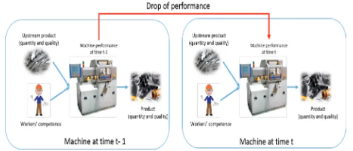
In this part, we will use an industrial example to present how the EOOBN can be used for modelling a large and repeatable system. The construction process follows five main steps which we will be successively described. The case study is a production workshop, composed of many machines or work centres (Figure 4). Within this organization, a machine receives products from upstream production work centres. Two dimensions are taken into account in this case. First, each machine brings an added value whose quality depends mainly on the quality of the input as well as the transformation which will be applied by the process. The latter rely itself on the machine performance as well as the worker skill (Figure 5). The second particularity of our case consists in assuming a gradual drop of performance of a machine over time due to weir and fatigue phenomena (Figure 6).

Fig. 4. Machine output influent parameters

Fig. 5. Machine communication

Fig. 6. Machine performance degradation

The main objective here is to simulate the drop of per-formance related to degradation due to ageing process of a three machine manufacturing line. Regarding a single machine, the good running will obviously depend on many variables such as upstream product quantity and quality, workers skills, as well as local machine characteristics. All

these variables interact to lower progressively the theoret-ical performance. The modelling procedure will follow the steps described in the above sections.

4.1 Formalize the structure of a system

In the manufacturing process which is composed by a production chain, the machine performance is the basic elements that may influence the productivity. Meantime the evolution mechanism (ageing for instance) of a pro-duction machine is a dynamic procedure. A propro-duction chain is built by a set of local machines. To simulate the productivity for a machine, we should consider not only the local machine performance but also the corresponding raw material or semi-finished product coming out from the preceding work centre. However we could construct a general model for all the machines which could present the performance evaluation mechanism of a production machine.

4.2 Design the structure of each class without considering the dynamic part

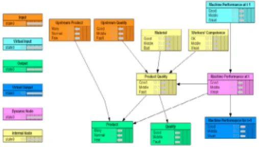
Following the construction method of the EOOBN and after analyzing the system, the structure of each class has now to be designed. In this case we have only one class, which is related to the machine performance. In Figure 7, we present the common structure for machine performance assessment. The basic elements in this class are:

• Input nodes: Upstream Product Quantity and Up-stream Product Quality

• Internal nodes: Material, Workers’ competence, Prod-uct quality and Machine Performance

• Output nodes: Product Quantity and Product Qual-ity

Fig. 7. Class: Representation of machine performance The upstream product quantity is an input node repre-senting the number of intermediate product which comes from the preceding work centre while the upstream quality shows the quality of the corresponding intermediate prod-uct. The output nodes correspond to the machine outcome which are the product quantity and quality. The internal elements in the class are characterized by the quality of the raw material and the aptitude of the worker to make his job properly.

4.3 Identify the dynamic variables and add the virtual nodes

For a local machine post, the machine performance which is an internal node in Figure 7 has to be considered as a dy-namic variable evolving with time. Consequently, a virtual Upstream product

(quantity and quality)

r

Workers' competence

Upstream product (quantity and quality)

I Workers'comp€tence Upstream product (quantity and quality) I Workers'competence Machine performance attimet Machine 1 MJchi~perfc.-m:in<e attimHI Machine at time t-1 Machine performance attimet Product (quant1tyandqua!1ty) Upstream product (quantity and quality)

I

Workers'competence

Drop of performance Up~treamproduct (quantity and quality)

I

Workers'competence

Product

(quantity and quality)

Machine performance attimet Machine 2 Machinepe,form.lnce attimet Machine at time t ls~eoqxrt!d ~ ~ 0

input characterizing the parent of machine performance at time t is added as well as a virtual output representing the communication channel with next time slice (Figure 8).

• Dynamic node: Machine performance at time t • Virtual nodes: Machine performance at time t − 1 as

the virtual input and Machine performance for time t + 1 as the virtual output

Fig. 8. Class: Representation of dynamic machine perfor-mance

Here we have two types of communication channel: the machine communication channel which is in charge of the information exchange from one product post to other one and the dynamic communication channel which is in charge of information exchange between time-slices for one machine post. In this case study, we suppose that the machine performance at time t depends only

on time t_{− 1. In case of more time-dependent variables,}

virtual inputs associated with the corresponding dynamic variables can be added as needed. These extra virtual inputs allws keeping the global network in a uniform representation (Figure 9). Table 1 presents the machine dynamic performance. The data is just for the simulation which is not from the real case.

4.4 Instantiate the class by introducing the parameters corresponding to the object

The parameters associated with the class are then to be set up to give rise to the corresponding objects. In Figure 8 the production line made of three machine posts is represented by an EOOBN model. Each object has one dynamic variable. The Quality variable has four parents and each parent has three states. The conditional probability table

of Quality has 34 _{= 81 raws with, for each one has three}

probability values.

4.5 Connect the objects through their communication channels

This step makes appear a 2 dimensional problem with first the machine connection characterizing the production flow and second the temporal connection representing the evolution of the dynamic variables. In the EOOBN infor-mation propagation, we should first connect the machine posts to have the whole production line and then consider the dynamic evolution see Figure 9.

4.6 Simulation results

The simulation is based on system made of three machines and twenty time-slices. There are ten nodes (variables) in

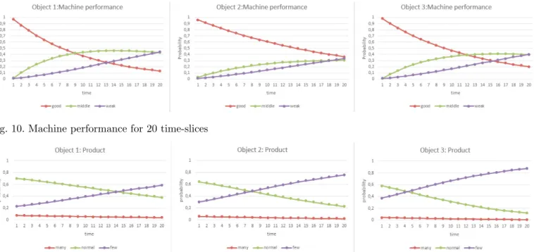
Fig. 9. An EOOBN model based dynamic production line each object, that is 30 variable in total for the description of the production line. Multiplied by 20 time-slices, this would lead to 600 variables in a classical Dynamic Bayesian Network. Through the EOOBN modelling, each object can be processed separately, keeping the computation size at 10 variables independently of the number of machines involved in the production line, Figure 10 and 11 show the simulation results related to the performance of the case study as well as the product generated by the system in the absence of maintenance. One can see clearly for each machine the gradual degradation of productivity and machine performance.

5. CONCLUSION AND PERSPECTIVES In this communication, we presented the construction method of a new modelling technique for complex systems with an Extended Object Oriented Bayesian Network as underlying tool. An EOOBN has been proposed to tackle modelling challenges raised by large scale and complex real world systems. An EOOBN turns out to be more powerful than classical OOBN by its capacity to both simplify the graphical representation of a system and reduce the com-putation size. Indeed, distinguishing classes and objects gives more flexibility for variation of parameters required for the representation of real systems. When a repetitive structure allows the use of such Object Oriented represen-tation, an EOOBN is undoubtedly suitable for modelling complex situations encountered in risk management frame-work. At the same time an EOOBN uses the virtual nodes to introduce the dynamic part into the class/object. An illustrative application in an industrial process has been used to show the interest of such modelling technique. In a future work, the inference algorithm will be used in a real world application and the learning techniques associated with such modelling will be considered.

REFERENCES

Amaral, L.A. and Ottino, J.M. (2004). Complex networks. The European Physical Journal B-Condensed Matter and Complex Systems, 38(2), 147–162.

Bangsø, O. and Wuillemin, P.H. (2000). Object oriented bayesian networks a framework for topdown specifica-tion of large bayesian networks and repetitive structures. Ben Hassen, W., Auzanneau, F., Incarbone, L., P´eres, F., and Tchangani, A.P. (2013). Omtdr using ber estima-tion for ambiguities cancellaestima-tion in ramified networks di-agnosis. In Intelligent Sensors, Sensor Networks and In-formation Processing, 2013 IEEE Eighth International Conference on, 414–419. IEEE.

Bouzarour-Amokrane, Y., Tchangani, A., and Peres, F. (2015). A bipolar consensus approach for group decision

Axis 1: Production Line

P (M Pt|MPt−1) machine 1 performance machine 2 performance machine 3 performance

good middle weak good middle weak good middle weak

good 90% 9% 0% 95% 4% 1% 92% 7% 1%

middle 0% 95% 5% 0% 95% 5% 0% 95% 5%

weak 0% 0% 100% 0% 0% 100% 0% 0% 100%

Table 1. Conditional probability table for the machine dynamic performance

Fig. 10. Machine performance for 20 time-slices

Fig. 11. Production for 20 time-slices

making problems. Expert Systems with Applications, 42(3), 1759–1772.

Godichaud, M., P´er`es, F., Gonzalez, V., Tchangani, A.,

Crespo, A., and Villeneuve, E. (2011). Integration

of warranty as a decision variable in the process of recertification of parts resulting from end-of-life system dismantling. In Quality and Reliability (ICQR), 2011 IEEE International Conference on, 156–160. IEEE. Godichaud, M., P´er`es, F., and Tchangani, A. (2012a).

Optimising end-of-life system dismantling strategy. In-ternational journal of production research, 50(14), 3738– 3754.

Godichaud, M., Tchangani, A., P´er`es, F., and Iung, B. (2012b). Sustainable management of end-of-life systems. Production Planning & Control, 23(2-3), 216–236. Jaeger, M. (2000). On the complexity of inference about

probabilistic relational models. Artificial Intelligence, 117(2), 297–308.

Kamissoko, D., P´er`es, F., and Zarat´e, P. (2011). Infras-tructure network vulnerability. In International con-ference on collaboration technologies and infrastructures (WETICE), 2011, pp–305.

Koller, D. and Pfeffer, A. (1997). Object-oriented bayesian networks. In Proceedings of the Thirteenth conference on Uncertainty in artificial intelligence, 302–313. Morgan Kaufmann Publishers Inc.

Langseth, H. and Bangsø, O. (2001). Parameter learning in object-oriented bayesian networks. Annals of Mathe-matics and Artificial Intelligence, 32(1-4), 221–243. Langseth, H. and Nielsen, T.D. (2003). Fusion of domain

knowledge with data for structural learning in object oriented domains. The Journal of Machine Learning

Research, 4, 339–368.

Liu, Q., Tchangani, A., and P´er`es, F. (2016).

Mod-elling complex large scale systems using object oriented bayesian networks (oobn). IFAC-PapersOnLine, 49(12), 127 – 132.

Liu, Q., Tchangani, A., Kamsu-Foguem, B., and P´er`es,

F. (2015). Modelling a large scale system for risk

assessment. In Industrial Engineering and Systems

Management (IESM), 2015 International Conference on, 203–208. IEEE.

Murphy, K.P. (2002). Dynamic bayesian networks: repre-sentation, inference and learning. Ph.D. thesis, Univer-sity of California, Berkeley.

Nielsen, T.D. and Jensen, F.V. (2009). Bayesian networks and decision graphs. Springer Science & Business Media.

Pearl, J. (1988). Probabilistic reasoning in intelligent

systems: networks of plausible inference. Morgan Kauf-mann.

P´er`es, F. and Grenouilleau, J.C. (2002). Initial spare parts supply of an orbital system. Aircraft Engineering and Aerospace Technology, 74(3), 252–262.

Rabiner, L. and Juang, B.H. (1986). An introduction to hidden markov models. ASSP Magazine, IEEE, 3(1), 4–16.

Weber, P. and Jouffe, L. (2006). Complex system relia-bility modelling with dynamic object oriented bayesian

networks (doobn). Reliability Engineering & System

Safety, 91(2), 149–162.

Wuillemin, P.H. and Torti, L. (2012). Structured proba-bilistic inference. International Journal of Approximate Reasoning, 53(7), 946–968. 1 0,9 0,8 Z: 0,7 :2i 0,6 ] 0,5 e o,4 o.. 0,3 0,2 0,1 0,8

i

i

II

I

I

II

I

I

II

I

Object 1:Machine performance

1 2 3 4 5 6 7 8 9 ill 1112 D M 15 ffi U 18 D m

time

- - -good - . - .mddle - . - .weak

Object 1: Product

1 2 3 4 5 6 7 8 9 W 11 U UM 15 16 17 18 D W

time

Object 2:Machine performance

1

~:

~

~

~::

i

1 2 3 4 5 6 7 8 9 ill 11 ll U 14 15 ffi 17 ffi H m

time

- . -good - . - .middle - . -weak

Object 2: Product 1 2 3 4 5 6 7 8 9 W 1112 13 M 15 16 17 18 D W time 1 0,9 0,8 Z: 0,7 :5 0,6 ~ 0,5 e o,4 o.. 0,3 0,2 0,1

Object 3:Machine performance

1 2 3 4 5 6 7 8 9 W 11 U 13 14 B 16 17 IB H m

time

- . -good ----middle - . -weak

Object 3: Product

1 2 3 4 5 6 7 8 9 ill ll U D M B ffi U IB D ~

time