Intergranular stress corrosion cracking of ion irradiated 304L stainless steel in PWR environment

(1)

DOCTORAT DE L'UNIVERSITÉ DE TOULOUSE

Délivré par :

Institut National Polytechnique de Toulouse (INP Toulouse) Discipline ou spécialité :

Science et Génie des Matériaux

Présentée et soutenue par :

Mme JYOTI GUPTA

le jeudi 7 avril 2016

Titre :

Unité de recherche : Ecole doctorale :

INTERGRANULAR STRESS CORROSION CRACKING OF ION

IRRADIATED 304L STAINLESS STEEL IN PWR ENVIRONMENT

Sciences de la Matière (SDM)

Centre Interuniversitaire de Recherche et d'Ingénierie des Matériaux (C.I.R.I.M.A.T.) Directeur(s) de Thèse :

M. ERIC ANDRIEU MME LYDIA LAFFONT

Rapporteurs :

M. JÉROME CREPIN, MINESPARISTECH

M. VIVEKANAND KAIN, ATOMIC RESEARCH CENTRE MUMBAI Membre(s) du jury :

1 M. PHILIPPE PAREIGE, UNIVERSITE DE ROUEN, Président

2 M. BENOIT TANGUY, CEA SACLAY, Membre

2 M. ERIC ANDRIEU, INP TOULOUSE, Membre

2 M. JOËL ALEXIS, ECOLE NATIONALE D'INGENIEUR DE TARBES, Membre

2 Mme LYDIA LAFFONT, INP TOULOUSE, Membre

(2)

(3)

Firstly, I would like to express my sincere gratitude to my advisors Prof. Eric Andrieu, Prof. Lydia Laffont and Dr. Benoit Tanguy for providing me the opportunity to work on such an interesting topic. I would like to thank Dr. Jérémy Hure for showing interest in my work and providing necessary guidance in times of hardship. I could not have imagined having better mentors for my PhD study. Their continuous support, patience, immense knowledge and motivation have helped me in all the time of research and writing of this thesis.

I would like to thank Prof. Philippe Pareige for accepting to head my dissertation committee. I would like to extend my gratitude to all the members of committee, Dr. Jérôme Crepin, Prof. Vivekanand Kain, Prof. Joël Alexis and Stéphane Perrin not only for their time and patience, but also for their insightful comments and encouragement which contributed to my development as a scientist.

During the thesis, I got the opportunity of working in Toulouse (CIRIMAT) as well as in Paris (CEA Saclay). I am glad that I got the chance to meet many people with varied skills at both places. I would like to thank all my colleagues of CIRIMAT and CEA for their encouragement and assistance. Special thanks to Clement Berne, Deni Ferdian, Tristant Jezequel and Vincent Mcdonalds for bearing me and answering all my relevant or irrelevant questions patiently. For their assistance during irradiation campaign, I would like to thank Yves Serruys, Eric Bordas and team JANNuS (DMN/SRMP/JANNUS). I am indepted to Marie-Christine Lafont, who taught me about the TEM sample preparation techniques and spent numerous hours on TEM to get beautiful pictures of “defects” for my thesis. I would also like to acknowledge Matthias Rousseau and Holande Aurore (DPC/LECA) for carrying out the mechanical tests. I would like to thank Sylvie Poissonnet (DMN/SRMP) and Joël Alexis (INP-Tarbes) for conducting nano-hardness tests. For his supervision and guidance during FIB sessions, I would like to acknowledge Mickel Jublot (DMN/LM2E). I would like to thank Francoise Barcelo (DMN/SRMA) for conducting EBSD analysis. I would also like to thank team MEMO of CIRIMAT, SEMI of CEA.

Last but not the least, I would like to express my heartfelt gratitude to my parents (Mukesh Kumar and Hemlata Gupta) and brother (Pulkit Gupta) for their confidence and continuous support. Finally, there are my friends (Neetu Gupta and Nitendra Singh) with whom I was able to talk happily and endlessly about anything other than my research. Thanks for being that “zaroori” friend.

(4)

(5)

Dedicated to Mumma, Papa,

Pulkit and boss

(6)

2.2.3. MICROSTRUCTURE ... 78 2.2.3.1. EBSD ANALYSIS ... 79 2.2.3.2. TEM OBSERVATIONS ... 83 2.2.4. MECHANICAL PROPERTIES ... 87 2.2.4.1. HARDNESS ... 87 2.2.4.2. TENSILE PROPERTIES ... 91 2.3. IRRADIATED MATERIAL ... 92 2.3.1. IRRADIATION CONDITIONS ... 92 2.3.1.1. PROTON IRRADIATION ... 93

2.3.1.2. SELF ION IRRADIATION ... 95

2.3.2. MICROSTRUCTURE CHARACTERIZATION ... 98

2.3.2.1. PROTON IRRADIATION ... 99

2.3.2.2. SELF ION IRRADIATION ... 101

2.3.3. HARDNESS ... 104

2.3.3.1. NANO-HARDNESS ... 106

2.3.4. COMPARISON WITH LITERATURE ... 112

2.4. CONCLUSIONS ... 116

CHAPTER 3. IMPACT OF IRRADIATION ON IGSCC OF AUSTENITIC STAINLESS STEEL ... 121

3.1. INTRODUCTION ... 121

3.2. CRACKING OF ION IRRADIATED AUSTENITIC STAINLESS STEEL ... 122

3.2.1. QUALITATIVE ANALYSIS ... 123

3.2.2. QUANTITATIVE ANALYSIS ... 127

3.2.2.1. LOCALIZED DEFORMATION ... 131

3.2.2.2. CHARACTERIZATION OF OXIDE FORMED ON TENSILE SAMPLES ... 136

3.3. OXIDATION OF IRRADIATED AUSTENITIC STAINLESS STEEL ... 139

3.3.1. EFFECT OF IRRADIATION ON OXIDE FORMED ON AUSTENITIC STAINLESS STEEL .. 140

3.3.2. IMPACT OF VOLUME OF CORROSIVE MEDIUM ... 147

3.4. INFLUENCE OF DEFORMATION MECHANISM ON CRACKING MECHANISM OF IRRADIATED AUSTENITIC STAINLESS STEEL ... 149

3.4.1. MORPHOLOGY OF THE CRACKS OBSERVED... 149

3.4.2. VALIDATION OF CRITERION PROPOSED FOR INTERGRANULAR CRACKING ... 152

3.5. DISCUSSIONS ... 159

3.6. CONCLUSIONS ... 165

CHAPTER 4. EFFECT OF SURFACE FINISH ON THE CRACKING SUSCEPTIBILITY ... 170

4.1. INTRODUCTION ... 170

4.2. IMPACT ON CRACKING SUSCEPTIBILITY ... 171

(8)

4.2.3. LOCALIZED DEFORMATION... 176

4.3. OXIDATION KINETICS ... 178

4.3.1. IMPACT OF SURFACE FINISH ON THE OXIDATION OF AUSTENITIC STAINLESS STEEL 179 4.3.2. IMPACT OF IRRADIATION ON OXIDATION OF MECHANICALLY POLISHED AUSTENITIC STAINLESS STEEL ... 182

4.4. DISCUSSION ... 184

4.5. CONCLUSIONS ... 188

CHAPTER 5. IMPACT OF LOADING CONDITIONS ON IGSCC OF IRRADIATED AUSTENITIC STAINLESS STEEL IN PWR ENVIRONMENT ... 192

5.1. INTRODUCTION ... 192

5.2. IMPACT OF LOADING CONDITIONS ON CRACKING ... 194

5.2.1. QUALITATIVE ANALYSIS ... 196

5.2.3. LOCALIZED DEFORMATION... 199

5.3. DISCUSSIONS ... 201

5.4. CONCLUSIONS ... 204

CONCLUSIONS AND FUTURE PERSPECTIVES ... 207

APPENDIX 1: SAMPLE MACHINING AND PREPARATION ... 211

A.1.1. MACHINING ... 211

A.1.2. SAMPLE PREPARATION ... 212

A.1.2.1. IRRADIATION ... 212

A.1.2.2. TRANSMISSION ELECTRON MICROSCOPE (TEM) ... 213

A.1.2.2.1. MICROSTRUCTURAL CHARACTERIZATION ... 213

(9)

Figure 1: a) Diagramme représentant la contribution des différentes ressources d'énergie dans la production totale d'énergie en France. b) Schéma illustrant la manière dont les cloisons sont reliées aux renforts par l'intermédiaire des vis. ··· xix Figure 2: Profil de dureté montrant la comparaison de la dureté obtenue pour les échantillons non irradiées (bleu), 5 dpa - Fe (en rouge) et 10 dpa - Fe (en vert) en utilisant les essais de nano indentation. ··· xxiii Figure 3: Augmentation de la dureté tracée en fonction de la densité des boucles de Frank pour toutes les doses d'irradiation ··· xxiv Figure 4: image MEB de la région irradiée de l’échantillon 5 dpa - Fe après l’essai SSRT réalisé en milieu REP. La direction de chargement est indiquée sur l'image. ··· xxv Figure 5: Image MEB dans la région irradiée de l’échantillon 5 dpa – Fe après l’essai de corrosion dans un environnement inerte jusqu'à la déformation plastique de 4%. La présence de lignes de glissement sur la surface de l'échantillon est clairement visible. Certains des joints de grains sont marqués par une ligne noire (en pointillés). La direction de chargement est indiquée dans l'image. ··· xxvii Figure 6 : Schémas illustrant la profondeur de la zone irradiée dans les échantillons 10 dpa - Fe et 10 dpa - Fe (mech.). Le profil de dommage est représenté en pointillé rouge et les joints de grains en bleu. ··· xxxi Figure 7: Images en champ clair obtenues au MET montrant les défauts d'irradiation observés dans l’ échantillon a) vibro-poli b) poli mécaniquement après l'irradiation au fer à une dose de 10 dpa. ··· xxxi Figure 8 : Micrographes MEB des échantillons non irradiés oxydés en autoclave pendant 360 h en milieu REP a) vibro-poli b) poli mécaniquement. ··· xxxiv Figure 9: a) Schéma illustrant le cycle de température pendant le fonctionnement normal et la période de maintenance (source EDF). b) Graphique de la contrainte en fonction du temps pour les conditions de chargement cycliques (en trait plein rouge) et constant (en traits pointillés bleu) utilisés. Pré-déformation appliqué avant le chargement est représenté en pointillé rouge. ··· xxxvi Figure 10: Baffle former assembly locations and views for a CP0 900 MWe PWR [4]. ··· 1 Figure 11: Intergranular cracks (indicated by arrows) observed on the neutron irradiated baffle former bolts of the PWRs [source EDF]. ··· 2 Figure 12: Summary of the inspection results for baffle bolts of CP0 PWRs that have been confirmed detective [6]. 3 Figure 13: Few modifications incorporated in the design of baffle bolts to suppress cracking in PWR environment [7]. ··· 3 Figure 14: Venn diagram of the factors contributing to the Irradiation Assisted Stress Corrosion Cracking of the material [3]. ··· 4 Figure 1-1 : Venn diagram to represent the different factors contributing in the IGSCC of material [25]. ··· 6 Figure 1-2 : Schematic depicting all possible mechanistic issues believed to influence crack advance during IASCC of austenitic stainless steels in LWRs [6]. ··· 6 Figure 1-3 : Conditions necessary for Stress Corrosion Cracking [7]. ··· 7 Figure 1-4 : Schaeffler – DeLong diagram [1]. ··· 10 Figure 1-5 : Schematics representing the evolution of outer and inner oxide of 316 SS in PWR environment with time of exposure [28]. ··· 14 Figure 1-6 : a) Oxide thickness (for polished surface) plotted as a function of exposure time [29] b) effect of crystallographic orientation apparent on 316 L samples after an oxidation of 24 h in PWR environment [28]. 14 Figure 1-7 : Schematics illustrating the oxide formed on 304 L sample under simulated PWR primary water at 340 °C for 500 hours: a) polished surface b) ground surface [30]. ··· 15 Figure 1-8 : Evolution of inner oxide thickness as a function of cumulated deformation [32]. ··· 16 Figure 1-9 : SEM image of a) the crack observed b) zoomed image indicating the slip step like pattern observed in SUS 316 SS post to CERT in PWR environment [24]. ··· 18 Figure 1-10 : Fission spectrum in a Pressurized Water Reactor [41]. ··· 21 Figure 1-11 : Defects in the lattice structure of materials that can change their mechanical properties [44]. ··· 23 Figure 1-12 : Defects reported to be observed in austenitic stainless steel as a function of irradiation dose and temperature [6]. ··· 24 Figure 1-13 : a) Diffraction condition to obtain rel –rod image of one of the families of the Frank loops [55] b) A typical TEM Dark Field micrograph of the family of the Frank loops observed in SA 304L irradiated to 36 dpa at 390 °C in PHENIX Fast Breeder reactor (FBR) [55]. ··· 26 Figure 1-14 : Evolution of faulted Frank loops density with irradiation temperature in a neutron irradiated austenitic stainless steel [49]. ··· 27

(10)

Figure 1-15 : Evolution of Frank loops density with dose in neutron irradiated austenitic stainless steel for different irradiation temperatures [6, 49 - 53]. ··· 28 Figure 1-16 : Frank loop size distribution in a) 304 SS b) 316 SS for different doses irradiated at an in-core position at 275 °C in the Barsebäck BWR [50]. ··· 28 Figure 1-17 : Evolution of Frank loops density with dose for an irradiation temperature range of about 290 – 360 °C in different neutron irradiated austenitic stainless steel [6, 49, 50, 52 - 60]. ··· 29 Figure 1-18 : Evolution of Frank loops size with dose for an irradiation temperature range of about 290 – 360 °C in different neutron irradiated austenitic stainless steel [6, 49, 50, 52 - 58]. ··· 29 Figure 1-19 : a) A typical TEM image of the cavities observed in baffle former bolt of Tihange - 1 PWR [55] b) Effect of neutron irradiation temperature on the cavity density observed in austenitic stainless steel [49]. ··· 31 Figure 1-20 : a) TEM lattice image of SFE observed in high purity 304SS neutron irradiated at 1.2 dpa at 275 °C in Barsebäck BWR reactor [58]. b) Size distribution of Frank loops (dotted line) and SFTs (solid line) observed in SA 304L irradiated in BOR 60 FBR at 320 °C with a dose rate of 9.4 x 10-7 dpa/s at different doses [72]. ··· 32 Figure 1-21 : Schematics showing the flow of defects and changes in composition at sink for a) Interstitial association Segregation b) Inverse Kirkendall Segregation mechanisms of irradiation induced segregation [6]. 34 Figure 1-22 : Concentration Profile plotted as a function of distance from grain boundary observed in a baffle former bolt taken from Tihange PWR and irradiated to a dose of 10 dpa [50, 76]. ··· 35 Figure 1-23 : Concentration profile of a) Cr b) Ni of grain boundary in irradiated stainless steel plotted as a function of dose [76, 77]. ··· 35 Figure 1-24 : Enrichment of Cr, Ni and Si from matrix level at edge on Frank loops in PWR irradiated CW 316 SS [60]. ··· 36 Figure 1-25 : a) Temperature and dose regime where precipitation is observed in SA 316 irradiated in Fast neutron fission reactor [49]. b) BF TEM image of observed in a CW 316 baffle former bolt irradiated at 8.5 dpa at 300 °C in Tihange – 1 PWR [57]. ··· 37 Figure 1-26 : Evolution of Yield strength and total elongation with dose for solution annealed stainless steels neutron irradiated at 270 – 380 °C [77]. ··· 39 Figure 1-27 : Deformation mode map for 316 and 316 LN stainless steels in true stress – dose space [16]. ··· 41 Figure 1-28 : a) Dark Field image of coarse dislocation channels observed b) Average step spacing distribution obtained in 35 dpa neutron irradiated SUS 316 austenitic steel deformed at slow strain rate to 13 % plastic strain [89]. ··· 42 Figure 1-29 : Average step height in the slip channels in alloys with different SFE at two doses and strain levels [90].

··· 43 Figure 1-30 : Dependence of average channel height on a) dislocation loop density b) void density for different doses and strain rates [95]. ··· 43 Figure 1-31 : Comparison of the morphology of the outer oxide observed in a) unirradiated b) proton irradiated austenitic stainless steel after corrosion for 1024 h in simulated PWR primary water [23]. ··· 44 Figure 1-32 : Comparison of morphology of outer oxide (a – c) and thickness of inner oxide (d – f) in unirradiated, proton and xenon irradiated 316 L after corrosion for 600 h in simulated PWR primary water [98]. ··· 45 Figure 1-33 : Dependence of intergranular stress corrosion cracking in neutron-irradiated 304 SS and 316 SS as a function of neutron fluence in high dissolved oxygen water [77]. ··· 46 Figure 1-34 : Stress as percent of the irradiated yield stress vs. a) time b) dose for IASCC initiation in austenitic stainless steels in a PWR environment [extracted from 77]. ··· 47 Figure 1-35 : Stress vs. dose curve for IASCC initiation in austenitic stainless steels in a PWR environment indicating the different threshold stress curve for BFBs and FTTs [101]. ··· 48 Figure 1-36 : Schematic showing the increase in RIS, Frank Loop line length, hardness and SCC susceptibility with dose in PWR [33, 95]. ··· 49 Figure 1-37 : Removal of RIS, dislocation microstructure (measured by loop line length) and hardness as a function of iron diffusing distance (Dt). The data for the graph was taken from different studies conducted on neutron (BWR and PWR environment) and proton irradiated stainless steel (tested in BWR environment) [104]. ··· 50 Figure 1-38 : a) Cracks observed on in-service bolt b) Discontinuous cracking mechanism in PWR baffle bolt proposed by Thomas et al.. Crack proceeds in steps of brittle cracking along metal grain boundary followed by oxide formation to fill crack [82]. ··· 51 Figure 1-39 : Schematics illustrating a) rapidly growing crack in hydrogenated and oxygenated conditions b) arrested subcrack in deaerated conditions [108]. ··· 52 Figure 1-40 : Contribution of SFE, RIS, Hardness and Localized deformation to IASCC initiation. [95]. ··· 53

(11)

Figure 1-42 : Schematics representing the transfer of slip by dislocation channel to grain boundary resulting in the rupture of oxide film at the grain boundary and causing IGSCC [33]. ··· 54 Figure 1-43 : a) crack observed along a grain boundary with slip discontinuity in 73 dpa neutron irradiated austenitic stainless steel [106] b) schematic illustrating the interaction between dislocation channels and grain boundaries [89]. ··· 55 Figure 1-44 : Schematic representation of the Schmid law [18]. ··· 55 Figure 1-45 : Comparison of irradiation depth profile in austenitic stainless steel of Heavy ions and protons with neutron [112]. ··· 58 Figure 1-46 : Comparison of the dose dependence of a) Frank Loop density and b) size for austenitic stainless steel irradiated with neutrons at 270 – 340 °C and with protons at 360 – 400 °C and heavy ions at 300 – 500 °C [6, 47- 55, 65, 94, 95, 114 - 119]. ··· 61 Figure 1-47 : Comparison of grain boundary composition profile for CP 304L post to 5.5 dpa neutron irradiation in BOR-60 fast reactor (solid line) and 5.5 dpa proton irradiation at 360 °C (dashed line) [65]. ··· 61 Figure 1-48 : Comparison of the dose dependence of irradiation hardening for austenitic stainless steel irradiated with neutrons at 270 – 340 °C, and with protons at 360 °C and iron ions at 200 – 350 °C[61, 66, 119–124]. ·· 62 Figure 1-49 : a) Surface slip step morphology b) Average step height and spacing as a function of irradiation dose reported in SUS 304 after 2 MeV proton irradiation to 2.5 dpa at 300 °C and straining in argon at 300 °C to 2 % [121]. ··· 62 Figure 1-50 : Schematics representing the consequences of coupling of various parameters. Coupling of all four parameters i.e. susceptible material, irradiation, stress state and corrosive environment leads to IASCC. ··· 64 Figure 2-1: Comparison of the increase in hardness observed in 304 SS and 316 SS post neutron irradiation in a BWR at 275 °C [2]. ··· 75 Figure 2-2: Schematic to illustrate the original position of parallelepiped used to make samples (blue dashed parallelepiped) and orientation of sample machined along RT and TR directions from the parallelepiped in the 304L SS plate. ··· 78 Figure 2-3: IPF cartography indicating the austenite grain orientation along with ferrite phase (in black) in the SS 304L under study. ··· 79 Figure 2-4: View of the 3 faces indicating the anisotropic distribution of δ ferrite in the material used [4]. ··· 80 Figure 2-5: Estimation of the amount of ferrite using revised Schaeffler diagram (1990) [8]. The black circle indicates the SS 304 L grade under study [4]. ··· 80 Figure 2-6: Schematic illustrating the misorientation between two grains. ··· 81 Figure 2-7: Grain boundaries misorientation profile for virgin material obtained using EBSD analysis. ··· 82 Figure 2-8: EBSD image (post treatment with HKL software) indicating the presence of CSL boundaries in the material. In red are Ʃ3, in pink are Ʃ9 types (marked by black arrows) of CSL boundaries. Black dashed contours represent the δ ferrite and rests are the austenite grains. ··· 82 Figure 2-9 : BF TEM images of the ferrite with a) elongated b) ovoid morphology along with associated diffraction pattern. ··· 83 Figure 2-10 : BF TEM images (with associated diffraction pattern in inset) of Cr7C3 carbides (outlined using white

dashed lines) observed in the material. ··· 84 Figure 2-11 : BF TEM image of MnS precipitate (with associated diffraction pattern in inset) observed in the material. ··· 84 Figure 2-12 : a) Bright Field b) Dark Field TEM image (along with diffraction pattern) of mechanically polished sample indicating the presence of nanograins in the subsurface of the material. ··· 85 Figure 2-13: a) Austenite grains b) twins observed in the vibratory polished virgin material. ··· 86 Figure 2-14: a) Schematic to illustrate the placement of indents on the samples b) Example of Load – displacement profiles obtained for various indents made during nano indentation test. ··· 87 Figure 2-15: Examples of a) Hardness profile b) Corresponding Hardness² versus 1/d (or Nix – Gao) graph illustrating the estimation of extrapolated value, plotted for indents made on sample during nano indentation test. ··· 88 Figure 2-16: Nix and Gao plot of the vibro-polished material obtained from nano-indentation hardness tests performed on different machines. Value obtained from conventional Vickers test (after converting it to berkovich hardness value) is indicated as star in the figure. ··· 89 Figure 2-17: a) Hardness profile b) Nix and Gao plot showing the comparison of values obtained for mechanically polished (blue) and vibratory polished (red) materials using nano indentation test. ··· 90

(12)

Figure 2-18: Comparison of Cauchy stress – cumulative plastic strain graphs of initial material at 20°C and 340°C in air and at 340 °C in PWR environment. ··· 91 Figure 2-19: a) Samples placed on the copper stage during 2 dpa – H+ irradiation. Irradiation zone is indicated by yellow dashed square. b) Temperature profile for one of the sample obtained during the irradiation indicating the control of temperature within ± 10 °C. ··· 94 Figure 2-20: Damage profile for 2 dpa H+ irradiation (using 2 MeV, in blue) and for 1 dpa H+ irradiation (using 3.2 MeV, in red) in SS 304L obtained using SRIM-2011 under K-P approximation and using threshold displacement energy of 40 eV for Fe, Cr and Ni [15]. The irradiation dose at the 10 µm (indicated by arrow) was considered as the damage at irradiated surface.··· 95 Figure 2-21: a) Samples placed on the irradiation stage during Fe5+ irradiation at JANNuS Saclay. Irradiation zone is indicated by yellow dashed square and thermocouples are indicated by red arrows. b) Infra-red heat map indicating the temperature profile during the Fe irradiation ··· 96 Figure 2-22: Damage profile for 10 dpa (mech), 10 dpa Fe5+ irradiation (in blue) and for 5 dpa Fe5+ irradiation (in green) in SS 304L obtained using SRIM-2011 under K-P approximation and using threshold displacement energy of 40 eV [15]. ··· 97 Figure 2-23: Appm/dpa (KP) profile along with Damage profile for 10 MeV Fe ions and 1 MeV He ions in SS 304L obtained using SRIM-2011 under K-P approximation and using threshold displacement energy of 40 eV [15]. 98 Figure 2-24: Four families of Frank loops observed at a depth of 30 µm (~18 dpa K-P) on 1.0 dpa-H proton irradiated TENUPOL prepared sample along with diffraction pattern. ··· 100 Figure 2-25: a) Dark Field image of the Frank loops observed at the irradiation surface (~ 1 dpa K-P) b) cavities observed at the irradiation peak (~18 dpa K-P) in the 1 dpa-H proton irradiated sample. ··· 100 Figure 2-26: Bright Field TEM images showing a) the nano martensite grains (marked as M and Cr23C6 carbides

marked as X) along with associated diffraction pattern b) Irradiation induced defects observed in few nano austenite grains in the 10 dpa Fe (mech) irradiated samples. ··· 102 Figure 2-27 : a) Rel-rod DF TEM image b) High resolution BF TEM image along with Fourier transform (inset) of Frank loops observed in 5 dpa Fe sample. ··· 103 Figure 2-28: a) Bright Field TEM image indicating the size of few Frank loops observed b) size distribution of the Frank loops observed in 5 dpa Fe sample. ··· 103 Figure 2-29: BF TEM image of a) cavities observed in a nano austenite grain b) carbides (marked as C) with associated diffraction pattern which indexed it as Cr23C6. ··· 104

Figure 2-30: Schematic to show the position of the irradiation zone in the resin. ··· 105 Figure 2-31: a) Schematic to represent the indents made on the sample b) Actual image of the indents made during the nano indentation test to trace the irradiation damage profile. ··· 105 Figure 2-32: Comparison of proton irradiation damage profile traced by continuous stiffness measurement – nano indentation test performed on 1 dpa H sample at a depth of 500 nm with SRIM calculations. ··· 106 Figure 2-33: Comparison of Hardness profile for unirradiated and 1 dpa – H samples along with fitting lines to assess extrapolated values (black dashed lines) obtained using nano-hardness test. ··· 107 Figure 2-34: a) Image of the nano indent matrix in the unirradiated region obtained using optical microscope b) Evolution of the load as a function of indent penetration depth during nanoharness indentation tests. ··· 107 Figure 2-35: Comparison of Hardness profile of 2 dpa H and un-irradiated samples along with fitting lines to assess extrapolated values (black dashed lines) obtained using nano-hardness test. ··· 108 Figure 2-36: Hardness profile showing the comparison of hardness obtained for unirradiated (blue), 5 dpa – Fe (in red) and 10 dpa – Fe (in green) materials using nano indentation test. ··· 109 Figure 2-37: Comparison of Nix Gao plots of a) 5 dpa Fe, 10 dpa Fe b) unirradiated and 10 dpa Fe (mech.) samples obtained using nano-hardness test. ··· 110 Figure 2-38: Increase in hardness plotted as a function of density of Frank loops for all irradiation doses. ··· 111 Figure 2-39: Comparison of the Frank loops a) density b) size observed for proton (this study – red star) and iron irradiated (this study – blue stars) samples with neutron, proton and iron literature [9, 17 – 19, 20 – 37]. ··· 113 Figure 2-40: Comparison of the irradiation hardening observed in proton (this study – yellow star) and iron irradiated (this study – blue stars) samples with neutron, proton and iron literature [31, 35 – 40]. ··· 115 Figure 3-1 : Schematics to represent the irradiated area in the samples and bars. ··· 121 Figure 3-2 : Surface appearance of irradiated region of 5 dpa – Fe sample after SSRT test conducted in a) argon environment b) PWR environment. Loading direction is indicated on the image. ··· 123 Figure 3-3 : Surface morphology of a) unirradiated region b) irradiated region of 10 dpa – Fe sample and c) unirradiated region d) irradiated region of 2 dpa – H sample after SSRT test conducted in PWR environment.

(13)

Figure 3-4 : Surface cartography of irradiated areas of 5 dpa – Fe samples obtained using FSE depicting the intergranular nature of the cracks. Few cracks are marked by yellow arrows. Loading direction is indicated on the image. ··· 125 Figure 3-5 : Images to describe the FIB lift out sample preparation procedure used. a) Selecting a crack to be investigated and coating it with Pt deposit b) Milling the trenches on both sides of the crack c) Lifting the FIB prepared sample and gluing it on the TEM sample holder d) thinning of the sample using Ga ion beam. ··· 126 Figure 3-6 : a) SEM image prior to thinning b) EBSD phase orientation map of the FIB sample prepared from 5 dpa – Fe sample. Green indicated the FCC phase while red indicates the BCC phase. Grain boundaries are marked with white dashed lines and crack in b) is marked by black dotted line. Yellow dashed line (in a)) indicates the unirradiated – irradiated interface. Loading direction is indicated in the image. ··· 127 Figure 3-7 : SEM images of the same area of the irradiated zone of strained 5 dpa – Fe sample taken under a) SE mode b) BSE mode. The cracks in the region are marked by white arrows in both images. Loading direction is indicated in the image. ··· 128 Figure 3-8 : a) Schematics to demonstrate the preparation of the photomontage from the SEM images taken in the irradiated region of the strained samples b) Image to illustrate the criteria chosen to measure the crack length. ··· 128 Figure 3-9 : Crack length distributions obtained for unirradiated (in red) and irradiated (in blue) region of 5 dpa – Fe samples. Mean crack length is indicated by dashed line. ··· 129 Figure 3-10 : Crack length distributions obtained for 5 dpa – Fe (in blue), 10 dpa – Fe (in green), and 2 dpa – H (in red) samples. Mean crack length for each case is indicated by dashed line. ··· 131 Figure 3-11 : BSE-SEM image of the irradiated region of a) 5 dpa – Fe sample b) 2 dpa – H sample following straining in simulated PWR primary water upto 4 % plastic strain. The presence of slip lines on the surface of the sample is clearly visible. Some of the grain boundaries are marked by white dashed line. Loading direction is indicated in the image. ··· 132 Figure 3-12 : a) SEM images of slip lines observed in a) unirradiated region b) irradiated region of 5 dpa – Fe sample post to 4% plastic straining. The distance measured between two consecutive slip lines was considered as slip line spacing. Spacing between few slip lines is shown by green arrow in the images. ··· 133 Figure 3-13 : Slip line spacing distribution obtained for unirradiated (in red) and irradiated regions (in blue) of 5 dpa – Fe samples. The mean spacing for each case is indicated by dashes lines. ··· 133 Figure 3-14 : Slip line spacing distribution obtained for 5 dpa – Fe sample - tested in PWR environment (in blue) and tested in argon environment (in green). The mean spacing for each case is indicated by dashed line. ··· 134 Figure 3-15 : Comparison of slip line spacing distribution obtained for 5 dpa - Fe (in red), 10 dpa – Fe (in blue) and 2 dpa – H (in green) samples following straining in corrosive environment. The mean spacing for each case is indicated by dashed line. ··· 135 Figure 3-16 : Illustration of effect of irradiation depth on slip line morphologies. Red region represents the irradiated region of the grain. Red arrows point to the slip lines which originated in unirradiated matrix but were blocked by the irradiation damage [extracted from 9]. ··· 136 Figure 3-17 : Optical microscope image illustrating the difference in oxide formed on unirradiated and irradiated region of the strained sample. Blue arrow indicates the unirradiated – irradiated interface of the sample. ··· 137 Figure 3-18 : a) Bright Field (BF) TEM image of the oxide layers and substrate observed in unirradiated region of the strained 5 dpa – Fe sample. The inner layer is marked by white dashed line and the outer oxide crystallites are outlined in black dashed line. b) EDX Composition profile of Fe, Cr, Ni and O observed in the inner oxide and the substrate (along the red line in a) in the unirradiated region of strained 5 dpa – Fe sample. ··· 138 Figure 3-19 : a) BF TEM image of the oxide layers and substrate observed in irradiated region of the strained 5 dpa – Fe sample. b) EDX Composition profile of Fe, Cr, Ni and O observed in the outer oxide, inner oxide and the substrate (along the white line in a)) c) HRTEM images of one of the outer oxide crystallite along with Fourier Transform (in inset). d) HRTEM images of the inner oxide layer. The inner layer is marked by white dashed line and the outer oxide crystallites are outlined in black dashed line. ··· 139 Figure 3-20 : a) Schematics to show the hole made on the bars b) Photograph to illustrate the suspension of bars via zirconium wire. The samples were hanged on two different probes using screw. ··· 140 Figure 3-21 : SEM images of the surface of a) unirradiated b) 5 dpa – Fe irradiated c) 5 dpa – FeHe samples demonstrating the effect of irradiation on the morphology of oxide crystallites. ··· 141 Figure 3-22 : SEM image indicating the plausible impact of grain orientation (in the irradiated region) on the morphology of outer oxide crystallites formed on 5 dpa – Fe sample. ··· 142

(14)

Figure 3-23 : a) BF TEM images of oxide layer observed in unirradiated area b) and of one outer oxide crystallite (marked in red in a)) with the associated SAED pattern along the [011] zone axis. c) HRTEM image of the inner oxide and associated Fourier transform along the [011] axis. Inner oxide is marked by white dashed lines in b) and c). ··· 143 Figure 3-24 : a) Bright field image of the oxide layer observed on the 5 dpa – Fe sample. The two areas used to obtain HRTEM and BF STEM images are marked in red. b) HRTEM image showing the smaller crystallite of the outer oxide (in black dotted line) and the inner oxide (in white dashed line). c) BF STEM images combined with the EDX map analysis of c1) O c2) Cr, c3) Fe and c4) Ni showing the enrichment at the interface

oxide/substrate d) EDX profile of the O, Cr, Fe and Ni in the oxide layers and substrate of the sample. ··· 144 Figure 3-25 : a) Irradiation induced defects observed in the matrix of the oxidized 5 dpa – Fe sample. b) HRTEM image of the defects observed along the [011] axis within the austenite grain of the material. Some of the defects observed are indicated by white arrow and inner layer in b) is marked by black dashed line. ··· 145 Figure 3-26 : a) BF TEM image b) Zoomed image (red rectangle zone) of the oxides formed on the 5 –dpa FeHe sample. c) HRTEM image of inner layer combined with the Fourier transform (in inset) along the [011] zone axis. The inner layer was indexed to be spinel of type Fe, NiCr2O4. Outer layer is marked by black dotted line

and inner layer by white dashed line. ··· 145 Figure 3-27 : SEM images of the unirradiated region of 5 dpa – FeHe sample post to 360 hours oxidation in simulated PWR primary water environment in a) small b) big autoclave. ··· 147 Figure 3-28 : SEM images of the irradiated region of 5 dpa – FeHe sample post to 360 hours oxidation in simulated PWR primary water environment in a) small b) big autoclave. ··· 147 Figure 3-29 : TEM images of the irradiated regions of 5 dpa – FeHe sample post to 360 hours oxidation in simulated PWR primary water environment in a) small b) big autoclave displaying the differences in the outer oxide and inner oxides in the two samples. ··· 148 Figure 3-30 : SEM images depicting the various crack sites observed in iron (a – c) and proton (d) irradiated strained samples. a) Exemplify the slip continuity while slip discontinuity is illustrated in b). In c) and d) slip lines were present on both sides of the cracked grain boundary but did not satisfy the definition of continuous interaction. Few grain boundaries are marked by white dashed lines and slip lines are indicated by black dashed lines. Loading direction is indicated in the image. ··· 150 Figure 3-31 : SEM images depicting the crack sites observed in iron (a) and proton (d) irradiated strained samples where no visible slip lines were present on either sides of the cracked grain boundary. Few grain boundaries are marked by white dashed lines. Loading direction is indicated in the image. ··· 151 Figure 3-32 : Discontinuous cracks (some indicated by white arrows) observed in the irradiated region of strained a) 5 dpa – Fe b) 2 dpa – H samples. Slip lines are indicated by black dashed slip lines. Loading direction is indicated in the image. ··· 151 Figure 3-33 : Schmid factor a) map b) distribution obtained on a small area of the unirradiated region of 5 dpa – Fe sample after slow strain rate testing (4 % plastic deformation) in PWR environment. The different colours represent the different Schmid factor value of the grains. ··· 153 Figure 3-34 : Area of the irradiated region of 5 dpa – Fe sample after slow strain rate testing (4 % plastic deformation) in PWR environment shown as a) Schmid factor map with different colours representing different Schmid factor value of the grains and b) EBSD cartography obtained using FSE. Cracks are indicated by yellow arrow and ferrites are outlined in black. ··· 155 Figure 3-35 : Normalized distribution of Schmid Factor pairs of grains adjacent to the cracked grain boundaries observed in 5 dpa – Fe sample.··· 156 Figure 3-36 : Probability diagram to illustrate the percentage of the cracked grain boundaries observed to satisfy the given conditions in 5 dpa – Fe sample.··· 156 Figure 3-37 : a) EBSD cartography obtained using FSE b) SF mapping after 4% plastic strain in the irradiated area of 2 dpa – H sample. Cracks are indicated by yellow arrow and ferrites are outlined in black. ··· 157 Figure 3-38 : Normalized distribution of Schmid Factor pairs of grains adjacent to the cracked grain boundaries observed in 2 dpa – H sample. ··· 158 Figure 3-39 : a) SEM image (taken with a sample tilt of 30 °) of the crack chosen from the unirradiated sample to make FIB sample. b) SEM image of the FIB sample prepared by transverse cutting the crack shown in a). Loading direction is indicated in the image. ··· 160 Figure 3-40 : Comparison of crack length distribution obtained for 5 dpa – Fe, 10 dpa – Fe, 2 dpa – H samples (this study) with proton literature. ··· 161 Figure 3-41 : TEM images of the irradiated regions of a) 10 dpa – Fe b) 2 dpa – H samples displaying the difference in the morphology of outer oxide observed on two sample after 360 h oxidation test in 5L autoclave. Grains

(15)

Figure 4-1 : Schematics illustrating the extent of irradiated area in 10 dpa – Fe and 10 dpa – Fe (mech.) sample. Damage profile is shown in red (in dots) and grain boundaries are shown in blue. ··· 171 Figure 4-2 : SEM images taken under BSE (Back Scattered Electron) mode in a) unirradiated b) irradiated regions of 10 dpa – Fe sample and c) unirradiated d) irradiated regions of 10 dpa – Fe (mech.) sample after straining. Cracks are marked by white arrows. Loading direction is indicated in the figure. ··· 172 Figure 4-3 : Crack micrographs of irradiated region of a) 10 dpa – Fe (taken in BSE mode) b) 10 dpa – Fe (mech.) (taken in SE mode) samples after straining to 4% plastic strain in simulated PWR environment. Loading direction is indicated in the image. ··· 173 Figure 4-4 : Crack length distribution obtained for the unirradiated (in red) and irradiated (in blue) regions of 10 dpa – Fe (mech.) sample. ··· 174 Figure 4-5 : Crack length distribution obtained for the irradiated regions of 10 dpa – Fe (in blue) and 10 dpa – Fe (mech.) (in red). ··· 175 Figure 4-6 : BSE-SEM images of the irradiated region of a) 10 dpa – Fe b) 10 dpa – Fe (mech.) samples demonstrating the slip lines observed on the surface of these sample after straining. Few inter line spacing are indicated by white arrows. ··· 176 Figure 4-7 : Slip line spacing distribution for the unirradiated (in red) and irradiated (in blue) regions of 10 dpa – Fe (mech.) sample. Mean slip line spacing values for each region are indicated by dashed lines. ··· 177 Figure 4-8 : Slip line spacing distribution obtained for the unirradiated region of 10 dpa – Fe (in blue) and 10 dpa – Fe (mech.) (in red) sample. Mean slip line spacing values for each region are indicated by dashed lines.··· 178 Figure 4-9 : Comparison of the slip line spacing distribution obtained for the irradiated region of 10 dpa – Fe (in red), 10 dpa – Fe (mech.) (in blue) samples. Mean slip line spacing values are indicated by dashed lines. ··· 178 Figure 4-10 : SEM micrographs of a) unirradiated vibratory polished b) unirradiated mechanically polished samples oxidized in 0.38L stainless steel autoclave for 360 h in simulated PWR primary water environment. ··· 180 Figure 4-11 : Figure 4-11: BF TEM image of the unirradiated mechanically polished sample of a) the oxide formed, b) the recrystallized area (below the duplex layer) composed of nanograins c) EDX profile showing the evolution of chemical composition along the white line (in a) and d) duplex oxide layer showing the outer and the inner layer. ··· 181 Figure 4-12 : SEM images of the a) unirradiated b) 10 dpa – Fe (mech.) sample illustrating the difference in morphology of outer oxide crystallites observed on the two sample after oxidation in simulated PWR primary water for 360 h. ··· 183 Figure 4-13 : a) BF TEM image of the 10 dpa-Fe (mech.) and b) HRTEM image of the oxides combined with the FFT along the [001] zone axis obtained for the oxide formed on 10 dpa – Fe (mech.) sample. ··· 183 Figure 5-1 : Schematics illustrating the temperature cycle during normal working and maintenance period (source EDF). ··· 193 Figure 5-2 : Stress versus time graphs obtained for cyclic (in red solid line) and constant (in blue dashed line) loading conditions used. The tests were conducted at 340 °C in simulated PWR environment. ··· 195 Figure 5-3 : Schematics representing a) the pre-straining condition (in red dotted line) used prior to cyclic loading and b) strain versus time graph obtained for the cyclic loading condition used. ··· 195 Figure 5-4 : Schematics representing a) the pre-straining condition (in red dotted line) used prior to constant loading and b) strain versus time graph obtained for the constant loading condition used. ··· 195 Figure 5-5 : Comparison of true stress - strain graph obtained for SSRT and rapid loading condition used. The tests were conducted at 340 °C in simulated PWR primary water environment. ··· 196 Figure 5-6 : SEM micrographs obtained from the surface of a) 5 dpa – Fe_Cy (in BSE mode) and b) 5 dpa – Fe_Co (in SE mode). Few cracks are marked by white arrows. Loading direction is indicated in the figure. ··· 197 Figure 5-7 : SEM images (taken under BSE mode) of a) 10 dpa – Fe and b) 10 dpa – Fe_R samples after straining. Loading direction is indicated in the micrographs. ··· 197 Figure 5-8 : Crack length distributions obtained for 5 dpa – Fe_Cy (in blue) and 5 dpa – Fe_Co (in red) samples. · 199 Figure 5-9 : a) BSE SEM image obtained for 5 dpa – Fe_Co sample indicating the presence of slip lines following constant loading. b) Zoomed image of red rectangle in a). c) BSE SEM image obtained for 5 dpa – Fe_Cy sample. Grains marked 1 in b) and c) represents the grain with multiple slip system visible on the surface. Few slip lines of the two slip systems are marked by dotted lines. Loading direction is indicated in the figure. ···· 200 Figure 5-10 : Slip line spacing distribution obtained for 5 dpa – Fe_Cy and 5 dpa – Fe_Co samples. ··· 201 Figure 5-11 : Crack length distributions obtained for 5 dpa – Fe (in blue), 5 dpa – Fe_Cy (in red) and 5 dpa – Fe_Co (in green) samples. ··· 204

(16)

Figure 0-1 : Drawing of the samples (Tensile and Flat bars) a) for all irradiation campaigns b) for 2 dpa H irradiation

campaign fabricated with the designated measurements (in mm). ··· 211

Figure 0-2 : Schematics representing the machining direction of the samples. ··· 211

Figure 0-3 : Schematic to show the small cuboids cut from the bars for TEM samples preparation. ··· 213

Figure 0-4: Illustration of the parallelepipeds prepared by cutting the sample using diamond wire saw. ··· 214

Figure 0-5: Schematics demonstrating the preparation of thin slices from parallelepipeds. ··· 214

(17)

Table 1: Irradiation conditions of the core internals of a PWR [1]. ... 2

Table 1-1 : Chemical composition (in wt %) of 304L and 316L austenitic stainless steel as per ASTM standards [12]. ... 10

Table 1-2 : Mechanical properties (minimum values) of 304L and 316L austenitic stainless steel at room temperature as per ASTM standards [12]... 11

Table 1-3 : Slip systems possible in austenitic stainless steel (FCC) [18]. ... 12

Table 1-4 : Approximate time scale for the production of defects in irradiated metals [33]. ... 22

Table 2-1: Chemical composition of SS 304 L (in wt %) [4]. ... 77

Table 2-2: Mechanical properties of unirradiated SS 304L observed during tensile test performed in air and autoclave at 20 °C and 340°C... 92

Table 2-3: Summary of the ion irradiation temperature required to mimic the neutron equivalent damage. ... 92

Table 2-4: Different parameters for all proton irradiation campaigns conducted at 350°C ± 10°C. ... 94

Table 2-5: Different parameters for all the iron irradiation campaigns conducted at 450 ± 20 °C. ... 97

Table 2-6: Comparison of the irradiated microstructure observed for different doses in proton irradiated samples. 101 Table 2-7: Comparison of the irradiated microstructure observed in Fe irradiated samples. ... 103

Table 2-8: Comparison of irradiation hardening observed for different doses in material irradiated using different ions. ... 110

Table 2-9: Summary of irradiation induced microstructure, irradiation hardening observed in the material after proton and iron irradiation. ... 117

Table 3-1 : Summary of the quantitative analysis performed in the irradiated and unirradiated regions of 5 dpa – Fe, 10 dpa – Fe and 2 dpa - H samples. ... 130

Table 3-2 : Thickness of the oxide layers formed on unirradiated, 5 dpa – Fe and 5 dpa – FeHe samples following oxidation in simulated PWR primary water for 360 h... 146

Table 3-3 : Comparison of the oxide layers observed on 5 dpa – FeHe samples oxidized in simulated PWR primary water for 360 h in different autoclaves. ... 148

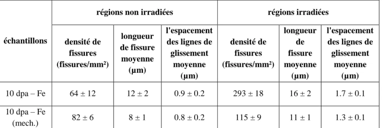
Table 4-1 : Comparison of the quantitative analysis performed in the unirradiated and irradiated regions of 10 dpa – Fe and 10 dpa – Fe (mech.) samples. ... 175

Table 4-2 : Comparison of the oxide layers formed on the vibratory polished and mechanically polished unirradiated samples after 360 h oxidation in simulated PWR primary water. ... 181

Table 4-3 : Comparison of the oxide layers formed on the unirradiated and 10 dpa – Fe (mech.) sample after 360 h oxidation in simulated PWR primary water. ... 184

Table 4-4 : Summary of quantitative analysis performed in the unirradiated and irradiated regions of 10 dpa – Fe and 10 dpa - Fe (mech.) samples... 189

Table 5-1 : Details about the designation of samples based on the loading condition used. Test duration and number of tests performed on each sample is detailed as well. ... 194

Table 5-2 : Comparison of the quantitative analysis performed on iron irradiated samples following different loading conditions. ... 202

(18)

ACRONYMS

APPM Atomic Parts Per Million APT Atom Probe Tomography

ASTM American Society for Testing and Materials BCC Body Centered Cubic

BF Bright Field

BFB Baffle Former Bolts BSE Back Scattered Electron BWR Boiling Water Reactor

CERT Constant Extension Rate Tensile CSL Coincident Site Lattice

CW Cold Work DF Dark Field

DPA Displacement Per Atom

EBSD Electron Back Scattered Diffraction EELS Electron Energy Loss Spectroscopy EDS Electron Dispersion Spectroscopy FBR Fast Breeder Reactor

FC Full Cascade

FCC Face Centered Cubic FFT Fast Fourier Transforms FIB Focused Ion Beam FP Frenkel Pair

FSE ForeScattered electron GB Grain Boundary

GDMS Glow Discharge Mass Spectrometry HFW Horizontal Full Width

HRTEM High Resolution Transmission Electron Microscopy IASCC Irradiation Assisted Stress Corrosion Cracking

ICP-AES Inductively Coupled Plasma Atomic Emission Spectroscopy and IGSCC Inter Granular Stress Corrosion Cracking

JIS Japanese Industrial Standards KP Kinchin and Pease

LAGB Low Angle Grain Boundaries LTO Long Term Operation

LVDT Linear Variable Displacement Transducer LWR Light Water reactor

NRT Norgett – Robinson – Torrens PIA Post Irradiation Annealing PIPS Precision Ion Polishing System PKA Primary Knock-on Atoms PT Pressure – Temperature PWR Pressurized Water Reactor

(19)

R&D Research and Development

RHAB Randomly High Angle Grain Boundary SA Solution Annealed

SAED Selected Area Electron Diffraction SCC Stress Corrosion Cracking

SCW Super Critical Water SE Secondary Electron

SEM Scanning Electron Microscope SF Schmid Factor

SFE Stacking Fault Energy SFT Stacking Fault Tetrahedra SHE Standard Hydrogen Electrode

SRIM Stopping and Range of Ions in Matter SS Stainless Steel

SSRT Slow Strain Rate Test

STP Standard Temperature and Pressure SUS Steel Use Stainless

TEM Transmission Electron Microscope TGSCC Trans Granular Stress Corrosion Cracking UHP Ultra High Purity

(20)

RESUME

En France, le secteur de l'électricité est dominé par l'énergie nucléaire, qui représente plus de 75% de la production totale d'électricité du pays. Le parc nucléaire électrogène français est constitué de réacteurs à eau pressurisés (REP). Ces dernières années, d’importants efforts ont été consentis pour prolonger la durée de fonctionnement des réacteurs de 40 à 60 ans.. Les structures internes du cœur du réacteur sont une partie essentielle des REP, car ils fournissent un support au cœur (ensembles combustibles et ’instrumentation) et elles canalisent la circulation du fluide caloporteur. L’intégrité de ces structures internes qui sont proches du combustible et en contact direct avec l'eau du circuit primaire doit être démontrée pendant toute la durée de fonctionnement du réacteur. Les aciers inoxydables austénitiques sont utilisés pour ces structures car ils sont résistants à la corrosion et en particulier à la corrosion sous contrainte. Les cloisons et renforts qui composent les structures internes sont constituées d’un acier austénitique hypertrempé 304 et / ou 304 L tandis que les vis sont constitués d’un acier 316 écroui (CW 316) et / ou 316 (CW 316L). Certains de ces composants, du fait de leur proximité avec le cœur, sont soumis à de fortes doses d’irradiation qui peuvent dépasser ~ 80 dpa (déplacement par atome) pour 40 années de service. Du fait du vieillissement des centrales nucléaires, ces composants accumulent des doses d’irradiation importantes et à terme peuvent devenir sensibles au phénomène de corrosion sous contrainte assistée par irradiation (IASCC). Plusieurs cas de défaillance de vis par IASSC ont été rapportés en France, en Belgique, et aux États-Unis (Figure 1). Bien que l'intégrité des internes puisse être garantie avec environ 1/3 des vis (sur un total d’environ 1000 vis), le temps de maintenance et l'optimisation des coûts au cours des inspections sont des problématiques importantes et ont conduit les opérateurs à s’intéresser à l’IASCC.

Figure 1: a) Diagramme représentant la contribution des différentes ressources d'énergie dans la production totale d'énergie en France. b) Schéma illustrant la manière dont les cloisons sont reliées aux renforts par l'intermédiaire des vis.

L’IASCC est un mécanisme de fissuration intergranulaire par corrosion sous contrainte (IGCSC) induite par l'irradiation. C’est un phénomène complexe qui se produit par la combinaison de

(21)

L'exposition aux neutrons est connue pour entraîner une modification de la microstructure et de la microchimie du matériau en induisant des défauts telle que des boucles de Frank, de la ségrégation induite par la radiation (RIS), de la précipitation et des cavités. Ces changements modifient les propriétés mécaniques du matériau. L’augmentation importante de la limite d'élasticité et la diminution de la ductilité avec l’irradiation ont été rapportées pour les aciers inoxydables austénitiques. Ces modifications induisent ou augmente la sensibilité à la CSC dans ces aciers en milieu REP Un seuil de fluence critique de ~ 2 ×1025 n/m² (≈ 3 dpa) à la fissuration a été proposé en dessous duquel 304 SS et 316 SS sont considérés comme immunes vis-à-vis de l’IASCC dans les REP.

Des recherches approfondies dans ce domaine ont montré que plusieurs facteurs (tels que la microstructure induite par l'irradiation, le durcissement par l’irradiation, RIS, etc.) contribuent à l’IASCC, mais aucun d'entre eux, n’est capable, seul, d'initier l’IASCC. L’effet prépondérant serait le mode de déformation des aciers inoxydables austénitiques irradiés et ces facteurs pourraient servir de contributeurs secondaires. A 300°C, la déformation se produit principalement dans des bandes de glissement. L'interaction de ces bandes avec les joints de grains est identifiée comme un facteur prépondérant dans l’amorçage des fissures dans le matériau irradié. Lorsqu'une bande de glissement interagit avec la surface libre ou avec les joints de grains, il en résulte la formation de marches. Ces marches sont caractérisées par la hauteur, la largeur et l'espacement et peuvent donner des informations quantitatives et qualitatives sur le degré de localisation de la déformation dans le matériau. Par ailleurs, la déformation localisée en environnement corrosif est identifiée comme une condition nécessaire pour la fissuration intergranulaire. L'irradiation peut également influer sur la chimie de l'eau, soit par radiolyse ou en modifiant la cinétique d'oxydation à la surface du métal. La radiolyse en milieu hydrogéné ne peut pas entraîner des changements importants dans le potentiel de corrosion et donc, n’apparait pas comme un facteur prépondérant pour l’IASCC en conditions REP. Cependant, les défauts induits par l’irradiation peuvent influencer la cinétique d'oxydation. Il a ainsi été montré que l’irradiation pouvait affecter la couche interne d’oxyde en modifiant son épaisseur et en induisant un enrichissement en Cr. Mais l'effet de l'irradiation sur la formation d’oxyde n’est pas encore clairement appréhendé et il reste encore un sujet ouvert à discussions.

Des études réalisées sur des échantillons irradiés aux neutrons ont servi d’étape préliminaire à l’identification des divers facteurs qui influent sur la sensibilité à la fissuration par IASCC. Mais, il reste encore des questions pour expliciter les mécanismes de dégradation et prédire leur évolution. Il est donc nécessaire d'effectuer des essais sur le matériau irradié en explorant divers facteurs sur une large gamme de dose d’irradiation et pour une large gamme de conditions (irradiation, chargement, environnement, etc.). La complexité associée à la conduite de caractérisations sur matériau irradié aux neutrons rend difficilement réalisable des études exhaustives. Les irradiations aux ions sont utilisées pour conduire des études analytiques sur les effets de l’irradiation. En utilisant des changements de température adéquats, l'irradiation aux

(22)

ions peut être un outil efficace pour isoler l'effet des divers paramètres dans l’IASSC. En effet, l'irradiation aux protons a été utilisée avec succès dans plusieurs études pour étudier la sensibilité à la fissuration du matériau dans différents milieux (REB, REP, environnement inerte). Cependant, peu d’études ont utilisé l'irradiation aux ions lourds.. Ainsi avec l’aide de la littérature actuellement disponible, nous avons mis l’accent, dans cette étude, sur le potentiel des ions lourds pour l’étude de l’IASCC.

L'objectif de cette thèse est d’étudier la fissuration intergranulaire par corrosion sous contrainte d’un acier inoxydable austénitique SA 304L irradié aux ions en milieu REP. Trois axes principaux ont été étudiés (i) l'impact de la microstructure induite par l'irradiation, (ii) l’impact de l’état de surface et (iii) l’effet du type de chargement mécanique sur la sensibilité de l’acier inoxydable austénitique 304L à la fissuration intergranulaire. Une méthodologie spécifique a été développée pour répondre aux objectifs de la thèse, qui comprenait la réalisation des irradiations, la caractérisation de la microstructure avant et après l’irradiation, suivis par des sollicitations mécaniques et les caractérisations de surface après ces dernières.

Un acier 304L hypertrempé (SA 304L) a été utilisé dans cette étude en raison de sa sensibilité à l’IGCSC légèrement plus élevée que le 316 et sa microstructure initiale simple par rapport à un acier écroui (état utilisé pour les vis de REP). Le matériau contient 19% en poids de Cr et 9 % en poids de Ni et l'énergie de défaut d'empilement (EDE) du matériau est de 23 mJ/m². La microstructure du matériau utilisé est constituée majoritairement d’austénite et d’une faible quantité de ferrite (~ 2 – 6%). La taille moyenne des grains est d’environ 27μm. Deux géométries différentes de échantillons ont été utilisées : des échantillons de traction (utilisés pour effectuer des essais mécaniques) et des barres (utilisées pour caractériser la microstructure, effectuer des essais de dureté et d'oxydation). La caractérisation de la surface par MET a révélé la présence de grains d'austénite de taille standard avec quelques grains de ferrite.

Les deux types d’échantillons ont été irradiés à JANNuS (CEA Saclay) en utilisant des ions 10 MeV Fe5+ à 450 °C avec deux doses différentes : 5 dpa et 10 dpa. Une irradiation complémentaire à 450°C en utilisant 10 MeV Fe5+ et 1 MeV He+ avec une dose de 5 dpa a également été réalisée. Avec cette énergie, la profondeur de pénétration des ions fer a été calculée à l’aide du logiciel SRIM. Elle est d’environ 2,5 µm. La région irradiée consiste en une zone dont le dommage croie continument avec un pic d'irradiation à environ 2 µm. En parallèle, une campagne d'irradiation aux protons a été réalisée au Michigan Ion Beam Laboratory (MBIL, Université du Michigan, USA) en utilisant des protons 2 MeV à 350 °C à une dose de 2 dpa. La région irradiée dans le matériau atteint une profondeur environ de 20 µm et se compose d'une région de dommage constante suivie par un pic d'irradiation à 19 µm. Le choix de la température pour les deux irradiations (fer et proton) a été choisi pour obtenir des microstructures et des mécanismes représentatifs de ceux observés pour des irradiations aux neutrons.

(23)

l’extrême surface d’irradiation alors que pour les échantillons irradiés aux protons, la caractérisation a été effectuée à l’extrême surface d’irradiation ainsi qu’au pic d'irradiation. La caractérisation a été réalisée en utilisant le MET et a révélé principalement la présence de boucles de Frank induites par l'irradiation pour les deux types d’irradiations.

La quantification de la densité des boucles de Frank a été réalisée sur 3 images différentes pour chaque dose. Pour estimer la densité, l'épaisseur moyenne supposée des lames minces est de 100 nm. Les résultats de cette évaluation quantitative sont détaillés dans le Table 1. La quantification de ces défauts est en bon accord avec la littérature pour les échantillons irradiés aux protons, ainsi que pour l’échantillon 10 dpa – Fe. Une densité plus faible d'un facteur 20 a été observée dans l'échantillon 5 dpa – Fe. Ceci est probablement dû à une sous-estimation de la densité des boucles de Frank. Cette hypothèse a été vérifiée en effectuant des mesures de densité de boucles de Frank sur l’échantillon 5 dpa – FeHe. Sur cet échantillon, une densité de 2,2 × 1022

boucles/m3 a été estimée ce qui est en bon accord avec la valeur déterminée pour l’échantillon 10 dpa – Fe et supérieur à la valeur de l’échantillon 5 dpa – Fe.

Irradiation Dommage (dpa K-P) densité des boucles de Frank (x 1022 m-3) Taille des boucles de Frank (nm) Augmentation du durcissement (%) 5 dpa – Fe 5 0,50 ± 0,31 13,4 ± 1,9 54 10 dpa – Fe 10 2,55 ± 1,05 14,9 ± 3,6 67 2 dpa – H 2 3,60 ± 1,50 13,8 ± 4,8 120

Table 1: Résumé de la microstructure induite par l'irradiation, du durcissement induit par l’irradiation observée dans le matériau après l'irradiation aux ions fer et aux protons.

Pour déterminer l'augmentation de la dureté sur l'échantillon irradié aux ions, un essaide nanodureté a été utilisé en raison des faibles profondeurs de pénétration des ions dans le matériau. Des indentations ‘Berkovich’ ont été réalisées à différentes profondeurs, et la dureté a été déterminée en utilisant la relation ‘Nix – Gao’ qui donne la courbe de la dureté² en fonction de l’inverse de la profondeur. Compte des interactions possibles entre les zones non irradiée et irradiée en fonction de la profondeur d’indentation, une attention particulière a été portée sur la détermination de la dureté pour les échantillons irradiés aux ions fer. Bien que la détermination de la dureté pour le matériau irradié aux ions fer ait été effectué jusqu’à une profondeur d'irradiation de 2,5 µm, seuls les résultats de l'indentation à la profondeur de d ≤ 0,5 µm ont été utilisés afin d’éviter de prendre en compte une contribution de la partie non irradiée (Figure 2). Ces difficultés ne sont pas rencontrées pour l’échantillon irradié aux protons (profondeur d'irradiation ~ 20 µm) en raison de leur pénétration plus profonde.

L'augmentation relative de la dureté dans l’échantillon irradié aux ions fer est de 54 à 67%, ce qui est inférieur d'un facteur 2 par rapport à la littérature concernant l’irradiation aux neutrons pour

(24)

une dose similaire, mais en excellent accord avec la littérature concernant l’irradiation au fer. Une augmentation relative de 120 – 130% est observée dans l’échantillon irradié aux protons, ce qui est en bon accord avec la littérature concernant les neutrons et les protons. Le résumé de ces résultats est rapporté dans Table 1. En utilisant d’une part un modèle de durcissement de type « barrière dispersée » pour évaluer l’augmentation de la limité d’élasticité et d’autre part et en évaluant l'augmentation de la limite d’élasticité à partir des valeurs de dureté mesurées, une corrélation linéaire entre l'augmentation de la dureté mesurée et la racine carrée du produit de la densité et de la taille des boucles de Frank induit par l’irradiation est obtenue (Figure 3).

Figure 2: Profil de dureté montrant la comparaison de la dureté obtenue pour les échantillons non irradiées (bleu), 5 dpa - Fe (en rouge) et 10 dpa - Fe (en vert) en utilisant les essais de nano indentation.

Une différence de dureté a été observé pour les échantillons irradiés 10 dpa – Fe et 2 dpa – H alors que la densité des boucles de Frank est similaire. Une explication potentielle est le rôle des défauts dont la taille est inférieure à la résolution du moyen de caractérisation (MET) utilisé dans cette étude. Il a été suggéré que la densité de ces défauts était plus élevée dans l’échantillon 2 dpa – H conduisant à une augmentation de la dureté plus importante. Mais la validité de cette hypothèse doit être vérifiée à l'aide d'outils de modélisation tels que la dynamique moléculaire, la cinétique de Monte Carlo et de la dynamique d’amas.

Les résultats de la caractérisation des microstructures et de la mesure de dureté ont suggéré que les conditions d'irradiation au fer, utilisées dans cette étude, étaient appropriées pour imiter l'irradiation ionique rapportée dans la littérature. Le défi était de vérifier la possibilité d'utiliser l'irradiation au fer pour étudier l'effet des dommages induits par l'irradiation sur la sensibilité à la

(25)

échantillons de traction irradiés ont été soumis à des essais de traction lente SSRT (Slow Strain Rate Test) dans différents environnements et les essais ont été interrompus après une déformation plastique de 4%.

Figure 3: Augmentation de la dureté tracée en fonction de la densité des boucles de Frank pour toutes les doses d'irradiation

 Possibilité d'utiliser l'irradiation au fer pour étudier la fissuration inter granulaire de l'acier inoxydable austénitique irradié.

Tout d'abord, l’essai a été effectué sur l’échantillon 5 dpa – Fe à la fois en environnement inerte (argon) et en milieu corrosif (milieu REP). La surface des échantillons a été analysée à l'aide du MEB. Sur la surface de l'échantillon testé dans un environnement inerte, aucune fissure n'a été observée. Alors que dans la région irradiée de l'échantillon testé dans l'environnement corrosif, de nombreuses fissures ont été observées (Figure 4). Ce résultat, montrant que l'environnement corrosif est une condition préalable indispensable à la fissuration inter granulaire de l'acier inoxydable austénitique 304L irradié à faible dose, était attendu.

Comme toute la longueur des échantillons de traction n’a pas été irradiée, une analyse de surface a été réalisée dans la région non irradiée des échantillons pour observer les fissures (le cas échéant). La majeure partie de la zone non irradiée de l’échantillon 5 dpa – Fe ne présentait aucune fissure. Cependant, une inspection approfondie a révélé la

(26)

présence de quelques petites fissures intergranulaires. Par la suite, les échantillons 10 dpa – Fe et 2 dpa – H ont été également testés en et analysés en utilisant le MEB. Dans les deux échantillons, quelques fissures ont été observées dans la région non irradiée alors que de nombreuses fissures ont été observées dans les régions irradiées. La nature de ces fissures inter granulaires a été déterminée grâce à plusieurs cartographies de surface dans la région irradiée en utilisant le système d'imagerie FSE (Forescattered Electron) de l’EBSD. En outre, et une coupe transversale a été réalisée par FIB et analysée à l'aide de l’EBSD sur une fissure choisie dans la région irradiée de l’échantillon 5 dpa – Fe. L'analyse a confirmé le nature inter granulaire de la fissure analysée.

Figure 4: image MEB de la région irradiée de l’échantillon 5 dpa - Fe après l’essai SSRT réalisé en milieu REP. La direction de chargement est indiquée sur l'image.

Pour des études comparatives, des informations quantitatives (à savoir la longueur et densité moyenne de la fissure) ont été déterminées. Une zone de 1 mm² (2mm x 0,5 mm) a été scannée dans la partie centrale de la région irradiée de l'échantillon en utilisant le MEB. La densité des fissures a été obtenue pour deux zones irradiées différentes. La densité moyenne des fissures et l'erreur ont été estimées. La longueur des fissures a été estimée à l'aide du logiciel ImageJ. Les résultats de l'analyse quantitative effectuée sur les échantillons sont résumés dans le Table 3-1. La reproductibilité de ces résultats a été confirmée en comparant la densité et la taille moyenne pour les deux ’essais SSRT sur échantillons irradiés 5 dpa – Fe.