Bond graph modeling for the simulation of an electromechanical chain

OATAO is an open access repository that collects the work of Toulouse

researchers and makes it freely available over the web where possible

Any correspondence concerning this service should be sent

This is an author’s version published in: http://oatao.univ-toulouse.fr/21671

To cite this version:

Trajin, Baptiste

and Vidal, Paul-Etienne

and Rotella,

Frédéric

Bond graph modeling for the simulation of an

electromechanical chain. (2018) In: International Conference on

Bond Graph Modeling and Simulation (ICBGM’2018), 9 July 2018

- 12 July 2018 (Bordeaux, France).

Bond Graph Modeling for the Simulation of an

Electromechanical Chain

Baptiste Trajin

Laboratoire Génie de

Production (LGP),

Université de Toulouse,

INP-ENIT,

Tarbes, France

[email protected]

Paul-Etienne Vidal

Laboratoire Génie de

Production (LGP),

Université de Toulouse,

INP-ENIT,

Tarbes, France

[email protected]

Frédéric Rotella

Laboratoire Génie de

Production (LGP),

Université de Toulouse,

INP-ENIT,

Tarbes, France

[email protected]

In complex multi-physic systems such as electromechanical chains, it is necessary to establish clear and simple simulation models. This need is linked to the increase of hardware in the loop (HIL) development processes. Indeed, this way of design complex systems allows to reduce development costs. However, HIL development efficiency is linked to the accuracy of models. Consequently, complex systems must be modeled using a comprehensive approach such as bond graphs leading to equations easily implementable on simulators. This paper proposes a model of a whole electromechanical chain including some nonlinearities of parameters leading to an accurate representation of real systems.

Author Keywords:

Bond Graph Models, Power electronics, Mechatronics, Simulation, Estimation.

I. INTRODUCTION

Bond graph method is a way to rapidly build a model of a whole system based on energy transfers [1], [2]. Using the principle of energy transfer, bond graph allows to represent any physical domains: mechanic, electricity, thermic, electromagnetic… Consequently, it is adapted to multi-physic representation of complex systems. Moreover, this model does not suppose linear behavior of variables and parameters. Due to characteristic equations of bond graph elements, state space representation of the system may be deducted. This state space representation allows to simulate and analyze systems using automatic tools.

This paper deals with the modelling and the simulation of a whole electromechanical chain. In the first section,

bond graph model of the power chain is established. Mechatronic and power electronics subsystems are particularly under concern. Nonlinear parameters are introduced depending on thermal behavior of the system and depending on internal variables. In section III, the state space representation of the whole system is deducted. Nonlinearities are taken into account in the mathematical expressions. These expressions lead to a simulation scheme of the electromechanical chain. Moreover, the simulation is able to represent harmonic behavior of the system and to integrate perturbations into the dynamic responses.

II. MODEL OF THE ELECTROMECHANICAL CHAIN A. Mechatronic subsystem

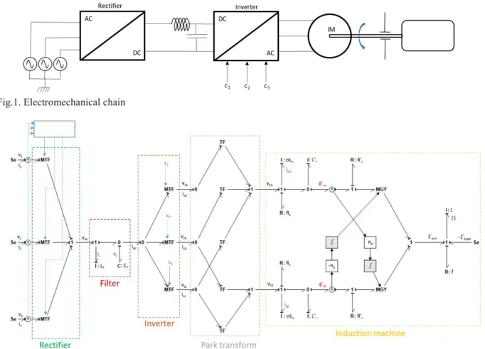
The considered electromechanical chain uses a three-phase squirrel cage induction motor (IM) supplied by an inverter (DC/AC converter). The input of the inverter is composed of a LC filter supplied by a diode bridge rectifier (DC/AC rectifier). The input of the rectifier is a three-phase alternative voltage network. The mechanical load of the motor is simplified to a global inertia applied to the motor axe, a friction proportional to the rotating speed and a constant torque load. The electromechanical chain is described in Fig. 1.

The different elements of the electromechanical chain are easily modeled using bond graph with integral causality [3]. Note that the induction motor is modeled in the Park coordinate system linked to the stator [4], [5]. Fig. 2 shows the whole bond graph model.

Obviously, gains of modulated transformers that model the inverter depend on the control of the inverter. Gains of modulated transformers that model the rectifier depend on the three-phase voltages. Parameters of the system are given in (1) [5].

Fig.1. Electromechanical chain

Fig. 2. Bond graph of the electromechanical chain !"# =$%& $' ! ("#= (#. )$% $'* + ,"#- =$_$%_'. ,#- (1) ,"#/ =$% $'. ,#/ 0 = 1 2 $%& $3.$'

where Lf and Cf are the filter’s inductance and capacitor,

Ls, Lr and Lm are respectively the stator, rotor and

magnetizing inductances of the induction motor, Rs and

Rr are respectively the stator and rotor resistances of the

motor, J is the inertia, f is the friction coefficient and Gload is a constant load torque.

B. Thermal subsystem

A thermal model of the motor has to be added. This model is based on RC thermal cells representing the different parts of the motor [6]. A simple thermal model is given in Fig. 3. Flow sources represent Joule losses in

the resistances of the induction motor and effort source represents the ambient temperature. Cth,r and Cth,s are the

thermal capacities of the rotor and the stator, Rth,r-s is the

conductive resistance between the rotor and the stator, Rth,s is the conductive and convective resistance between

the stator and the environment and Ta is the ambient

temperature of the environment. Temperatures of rotor and stator are respectively defined as Tr and Ts. Note that

Cth,r, Cth,s and Rth,r-s only depend on geometrical

parameters of the motor that are considered as constant and on materials properties (thermal conductivity, density and heat capacity) [7].

The thermal subsystem inputs are defined as follow: 456#= (#. 78#9+ : 8#++ : 8#;+<

456> = (>. 78>9+ : 8>++ : 8>;+< (2) where Is1, Is2, Is3, Ir1, Ir2, Ir3 represent respectively the

three-phases RMS currents of the stator and the rotor and PJ,r and PJ,s are Joule losses of the rotor and the

stator respectively.

C. Nonlinear parameters

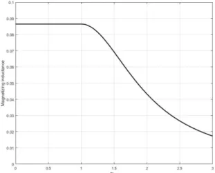
In the previous bong graph modelling, some nonlinear parameters are included, especially in the induction motor. As the induction motor is mainly composed of ferromagnetic materials, the magnetic field is submissive to saturation effects [8]. Magnetization is linked to magnetic field through the magnetizing inductance and geometrical parameters of the system. Consequently, the magnetizing inductance may depend on the magnetic flux value Lm(jr) and decreases with the

flux elevation. The variation law of Lm is defined in (3).

!? = !?6@ for ,#A ,9 !? = $%6B

9CDE'FEG_H%6B I& for ,# J ,9 (3) with ,_#= K,#-+ : ,_#/+ the amplitude of the rotor flux. The variation law of Lm in Fig. 4 is established in

accordance with results in [9].

Fig. 4. Magnetizing inductance of the induction motor Note that variations of magnetizing inductance Lm has

an effect on parameters L’r and R’r.

Moreover, electrical resistance of the stator and the rotor depends on temperature Rs(Ts), Rr(Tr), due to

temperature coefficient of Copper aCu and temperature

variations of stator DTs and rotor DTr (4) [10].

(>7L>< = (>6@. 71 : MNO. PT><

(#7L#< = (#6@. 71 : MNO. PT#< (4) where Rs,0 and Rr,0 stator and rotor are resistances at

ambient temperature.

Electrical resistances of the motor also may depend on frequency of currents. Indeed, skin effect appears in electrical conductors due to electromagnetic effects. This phenomenon becomes non negligible at high frequency. This skin effect has an impact on the electrical resistance [11] but this particular point is out of concern is this paper.

Finally, nonlinearity is introduced in the thermal model. Cooling of the motor is ensured by a fan linked to the rotor. Fluid mechanic equations (5) demonstrate that the convection thermal resistance Rcv included in Rth,s

depends on the rotating speed of the motor [12]. All other parameters in (5) are linked to air properties of geometrical parameters of the motor and depends on the design of the motor and its cooling system.

(QR7S< = U V6VWX. )Y. S. U_{Z. [} \]#* @.^ . 4_@.;;_{. `\]#. ZQR}! aaaaaaaaaaaaaa=ab Sc@.^ ₍₅₎

III. SIMULATION OF THE ELECTROMECHANICAL CHAIN

A. State equations

In order to simulate the whole system, a state space representation is built from the complete bond graph of the electromechanical chain (6). Note that expressions of functions f and h may be nonlinear.

de = f7d6 g<

h = i7d6 g< (6) State variables are defined as energy variables in integral causality, i.e. flow in I element and effort in C elements. Note that this method provides a low order state space representation. As a consequence, the limitation of differential equations is helpful for reducing the simulation duration through a lower computation complexity. Inputs of the state space representation in U are composed of effort and flow sources of the bond graph. Basically, outputs of the system in Y are the state variables in X.

1. Equations of the motor

According to Fig. 2, there are 5 state variables and then differential equations for the motor (7).

jk>-7l< jl =0. !1>. m2n(>7L>< : ( o_{#7,#6 L#<p. k>-7t<} :(o_!#7,#_o#7,#6 L_{< . ,}#< o #-7t< : qr. S7t<. ,o#/7t< : s>-7t<u jk>/7l< jl =0. !1>. m2n(>7L>< : ( o_{#7,#6 L#<p. k>/7t<} :(o_!o#7,##7,#6 L_{< . ,}#< o #/7t< 2 qr. S7t<. ,o#/7t< : s>/7t<u j,o #-7t< jl = (o#7,#6 L#<. k>-7t< 2( o_{#7,#6 L} #< !o#7,#< . ,o#-7t< 2 qr. S7t<. ,o #/7t<! j,o #/7t< jl = (o#7,#6 L#<. k>/7t< 2( o #7,#6 L#< !o#7,#< . , o #/7t< : qr. S7t<. ,o#-7t< vS7t< jl =1w . xqr. D,o#-7t<. k>/7t< 2 ,o#/7t<. k>-7t<I 2 f. S7l< 2 yz{\|7l<}

Obviously, previous state equations are nonlinear within the parameters and with multiplication of state variables due to:

- modulated gyrator in the induction motor model,

- Joule losses and the thermal model, - Flux dependency of magnetizing

inductance.

In addition to state equations (7), equalities has to be defined to evaluate rotor currents (8) needed to compute inputs of the thermal model.

ko #-7l< =~ •_'€7•< $•' 2 k>-7t< ! ko_{#/7l< =}~•'‚7•< $•' 2 k>/7t< ko_{#-7l< =} $' $%. k#-7l< (8)! ko_{#/7l< =} $' $%. k#/7l<

2. Equations of the filter

According to Fig. 2, there are 2 state variables in the filter model and then 2 differential equations (9).

|]H7ƒ< |ƒ = 9 $„. …2sQ7t< : s|Q7t<† |R‡7ƒ< |ƒ = 9 N„. …2k|Q7t< : k$7t<† (9) 3. Thermal equations

Equations (10) gives the state space equations associated to the bond graph of the thermal model in Fig. 3. State variables are temperature of the rotor Tr and the stator

Ts. Inputs are Joule losses and ambient temperature Ta.

jL#7l< jl =ˆƒ‰6#1 . m2 1 (ƒ‰6#c>. L#7t< : 1 (ƒ‰6#c>. L>7t< : (#7L#<. 78#9+ _{: 8#+}+ _{: 8#;}+_<u jL>7l< jl =ˆƒ‰6>1 . m 1 (ƒ‰6#c>. L#7t< 2 Š_(ƒ‰6#c>1 :_{(ƒ‰6>7S<‹ . L}1 >7t< :_{(ƒ‰6>7S< . L}1 \ : (>7L><. 78>9+ : 8>++ : 8>;+<u

B. Equations of non-differential elements

Non differential elements are subsystems without I or C elements in their bond graph model. In Fig. 2, the rectifier, the inverter and Park transform subsystems are non-differential. However, even if the electrical circuit structures do not vary along time, gains of modulated transformers are submissive to the values of efforts such as in the rectifier or to the control scheme for the inverter. For simulation purposes, control variables of the inverter c1, c2 and c3 are considered as input

parameters.

1. Rectifier equations

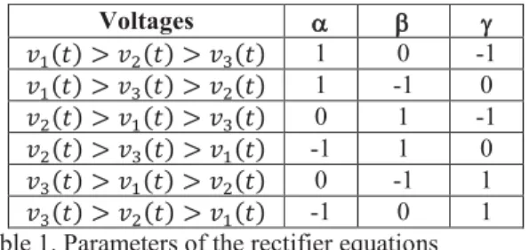
Gains of modulated transformers of rectifier equations depend on input effort values as seen in Table 1 [13], i.e. values of alternative input voltages (11).

s|Q7l< = M. s97l< : Œ. s+7l< : •. s;7l< ! k97l< = M. k$7l<

k+7l< = Œ. k$7l< (11)! k;7l< = •. k$7l<

2. Inverter equations

Gains of modulated transformers of inverter equations depend on control strategy and control signals c1(t), c2(t)

(7)

Voltages a b g s97l< J s+7l< J s;7l< 1 0 -1 s97l< J s;7l< J s+7l< 1 -1 0 s+7l< J s97l< J s;7l< 0 1 -1 s+7l< J s;7l< J s97l< -1 1 0 s;7l< J s97l< J s+7l< 0 -1 1 s;7l< J s+7l< J s97l< -1 0 1 Table 1. Parameters of the rectifier equations

and c3(t) of the inverter legs. In this simulation, the

control strategy of the inverter in 120° mode of conduction [13]. Equations of the inverter are given in equations (12). s>\7l< =9_;. …Ž. •97l< 2 •+7l< 2 •;7l<†. sQ7t< ! s>•7l< =9_;. …Ž. •+7l< 2 •97l< 2 •;7l<†. sQ7t< s>Q7l< =9_;. …Ž. •;7l< 2 •97l< 2 •+7l<†. sQ7t< ! k|Q7l< =9_;. …Ž. •97l< 2 •+7l< 2 •;7l<†. k>\7t< : aaaaaaaaaaaaaaaaa9_;. …Ž. •+7l< 2 •97l< 2 •+7l<†. k>•7t< : aaaaaaaaaaaaaaaaa9_;. …Ž. •;7l< 2 •97l< 2 •+7l<†. k>Q7t<

3. Park transform equations

The Park transform is expressed through a projection matrix Tpark and its pseudoinverse T+park (13) [14].

Ds_s>-7l<_{>/7l<I = L}r\#‘. ’ s>\7l< s>•7l< s>Q7l<“ a= ”Ž_{W .} • –1 2 1 Ž 21Ž V —_ŽW 2 —_{Ž ˜}W™ . ’ s>\7l< s>•7l< s>Q7l<“ ’k>\7l<k>•7l< k>Q7l<“ = Lr\#‘ C _{. Dk}>-7l< k>/7l<I (13) = ”Ž_{W .} • š – 1 V 21_Ž —W_Ž 21_{Ž 2}—W_{Ž ˜} › ™_{. Dk}>-7l< k>/7l<I C. Simulation algorithm

Regarding bond graph of the whole system in Fig. 2, inputs of electromechanical chain are three-phase supply voltages v1(t), v2(t) and v3(t) and load torque Gload(t). All other variables are either internal variables

needed for computation or state variables. The inverter

commands c1(t), c2(t) and c3(t) are considered as

parameters varying along time, leading to switched state space model [15], [16].

Regarding electrical and thermal parameters of the system, the simulation takes into account two different time steps. A short time step of dt1=0.1ms is considered

to solve electrical equations and a long time step of dt2=3s for thermal phenomena. On the one hand, the

variation of magnetizing inductance Lm(fr) is evaluated

for each short time step dt1. On the other hand, the

modification of resistances Rs(Ts) and Rr(Tr) due to

temperature elevation is realized at each long time step dt2.

The solving method chosen for differential equations is Heun’s method [17]. Let’s consider differential equation in (6). From a time instant j, an approximation of state X at time instant j+1 is given by (14) with dt the time step between the two time instants.

œ9= jl. fnd•6 g•p6

œ+= jl. fnd•: œ96 g•C9p (14) d•C9= d•:1_{Ž . 7œ}9: œ+<

D. Simulation results

During simulations, inputs of the mechatronic system are maintained constant: load torque, RMS value and frequency of three phase voltages v1(t), v2(t) and v3(t).

1. Averaged results

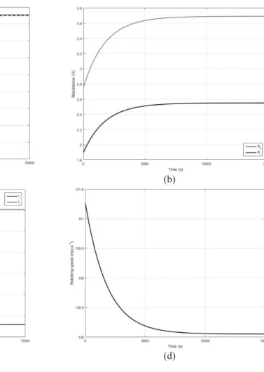
Fig. 5 shows the variation of main variables and parameters along time. Obviously, the temperature of the motor increases (Fig.5.a) due to Joule losses. This has with a direct effect on electrical resistances (Fig. 5.b) due to the positive temperature coefficient of Copper (4). As a consequence of the temperature elevation, stator (resp. rotor) averaged phase current slightly decreases (resp. increases) with a variation of about 1.3% (Fig. 5.c). The decrease of stator current can be interpreted by to the elevation of stator resistance at constant voltage. Simulations also shows an increase of magnetizing inductance, indicated a decrease of rotor flux. This can explain the decrease of rotor current. Finally, as the electromagnetic torque is linked to stator current and rotor flux, it decreases and the rotating speed of the motor also presents a decreasing tendency with a variation of 1.4% (Fig. 5.d).

2. Frequency components and casual analysis

Fig. 6 shows spectrum of stator phase current of the motor at the beginning and at the end of the simulation. To allow a clear harmonic comparison, spectra are (12)

(a) (b)

(c) (d) Fig. 5. Evolution of variables and parameters

Frequency (Hz) Amplitude at t=3s Amplitude at t=15000s Amplitude evolution

ŽžV -14.83dB -14.43dB +0.4dB WžV -27.31dB -26.84dB +0.47dB žžV -30.81dB -30.57dB +0.24dB XžV -35.83dB -35.33dB +0.5dB ŸžV -38.34dB -37.86dB +0.48dB žV -42.35dB -41.84dB +0.51dB

Table 2: Evolution of stator current harmonics

normalized and comparison of first harmonics is given in Table 2.

Regarding bond graph in Fig. 2, several causal loops are identified, one linking inductance and capacitor of the filter !¡¢ ˆ_¡, one linking filter capacitor and stator inductance of the motor nˆ¡¢ 0. !>p and one linking stator inductance and mechanical inertia 70. !>¢ w<. As there exists an action chain from input voltage to stator inductance of the motor, it becomes obvious that for a given voltage input, a modification of parameters of the motor such as magnetizing inductance, stator or rotor resistance has an impact on the transfer function linking variables. This transfer function has an impact on

harmonics amplitude of variables leading to the evolution that can be seen in Fig. 6 and Table 2. Similar results are obtained on input three-phase currents of the system.

IV. CONCLUSIONS

This paper deals with the use of bond graph to model a whole electromechanical chain. First of all, the mechatronic and thermal subsystems have been defined and studied to establish. Bond graphs of the system. From these bond graphs with nonlinear parameters, state space representation of the system have been defined. Considering differential and non-differential equations,

Fig. 6. Stator current spectrum

numerical simulations of the system have been performed. Simulations results clearly showed the evolutions of variables and parameters variations along time. Moreover, causal analysis has been achieved to justify the frequency content of variables. Finally, this simulation principle based on first-order differential equations could be implemented on real time simulators used for HIL development.

In further work, a more complete causal analysis will be performed to study the effect of different parameters on frequency content of state variables. Indeed, causal loops lead to transfer functions of the system and then to frequency behavior of variables. The work could also be completed with a study of effects of harmonic content of voltage inputs on different variables.

V. REFERENCES

[1] Borutzky W., “Bond Graph Modelling of Engineering Systems”, Springer, 2011

[2] Karnopp D. C., Margolis D. L., Rosenberg R. C., “System dynamics : modeling and simulation of mechatronic systems”, Wiley, 4th ed., 2006

[3] Gandanegara G., Roboam X., Sareni B., Dauphin-Tanguy G., “Modeling and Multi-time Scale Analysis of

Railway Traction Systems Using Bond Graphs”,

Proceedings of International Conference on Bond Graph Modeling and Simulation ICBGM'01, Phoenix, 2001 [4] Vas P., “Vector control of AC machines”, Oxford Science Publications, 1990

[5] Robyns B., François B., Degobert P., Hautier J. P., “Vector control of induction machines”, Springer, 2012

[6] Trajin B., Vidal P. E., Viven J., “Electro-thermal

model of an integrated buck converter”, European

Conference on Power Electronics and Applications (EPE’15 ECCE-Europe), 2015

[7] Bar-Cohen A., Kraux A. D., “Advances in thermal modeling of electronic components and systems”, ASME Press, 1988

[8] Chikazumi S., “Physics of ferromagnetism”, Oxford University Press, 2009

[9] Zaky M. S., Khater M. M., Yasin H., Shokralla S. S., “Magnetizing inductance identification algorithm for

operation of speed-sensorless induction motor drives in the field weakening region”, 12th International

Middle-East Power System Conference, 2008

[10] Kasap S. O., “Principles of Electronic Materials

and Devices”, 3rd ed., Mc-Graw Hill, 2006

[11] Canat S., Faucher J., “Fractional order :

frequential parametric identification of the skin effect in the rotor bar of squirrel cage induction machine”,

ASME Design Engineering Technical Conferences, 2003

[12] General Electric Company, “Heat transfer and fluid flow data book”, GE Compagny – Research and

Development Center, 1970

[13] Shepherd W., Zhang L., “Power converter

circuits”, Marcel Dekker, 2004

[14] Ben-Israel A., Greville T. N., “Generalized

inverses: theory and applications”, Springer, 2003

[15] Erickson R. W., Maksimovic D., “Fundamentals of Power Electronics”, 2nd ed. Springer, 2001

[16] Trampitsch S., Knoblinger G., Huemer M., “Switched State-Space Model for a Switched-Capacitor Power Amplifier”, IEEE International Symposium on Circuits and Systems, 2015

[17] Süli E., Mayers D., “An Introduction to Numerical Analysis”, Cambridge University Press, 2003

ABOUT THE AUTHORS

Baptiste Trajin, PhD, was born in 1982. He is now an Assossiate Professor of Electrotechnology at the Ecole Nationale d’Ingénieurs de Tarbes (ENIT) in France. He received the Eng. degree in electrotechnology and automation from the Ecole Nationale Superieure

d'Electrotechnique, d'Electronique, d'Informatique, d'Hydraulique et des Telecommunications, Toulouse, France in 2006. He obtained his M.S. and Ph.D degrees in electrical engineering from the Institut National Polytechnique de Toulouse in 2006, and from the Université de Toulouse in 2009 respectively. His research field was the diagnosis of electromechanical systems. From 2013, he is in the Laboratoire de Génie de Production of ENIT. He is currently working on modelling, estimation and diagnosis of multiphysics systems such as mechatronic systems and power electronic modules.

Paul-Etienne VIDAL obtained a Ph.D. degree (2004) from Institut National Polytechnique de Toulouse, France. From 2004 to 2006, he was engaged as Temporary Researcher at the laboratory LEEI, INPT/CNRS. Since 2006 he is an Associate Professor in the Laboratoire Genie de Production - Toulouse University. He obtained his Habilitation à Diriger des Recherches in 2017, from the INPT. His research topic deals with power converter efficiency. He developed 3 research themes within the PRIMES platform

(http://www.primes-innovation.com/) facilities: electro

thermo mechanical modeling and simulations; experimental technology integration for power electronic device; and control strategy of power converters.

Frédéric Rotella Senior Member (SM'96) of the IEEE Society, Frédéric Rotella was born in 1957. He received in 1981 the Engineer diploma from the Institut Industriel du Nord (Lille, France). From 1981 to 1994, he joined the Laboratoire d'Automatique et d'Informatique Industrielle de Lille where his research interests were focused on modelling, analysis and control of nonlinear systems. He received the Doctor Engineering degree and the Doctor of Physical Science degree respectively in 1983 and 1987 from the University of Science and Technology of Lille-Flandres-Artois. During this period, he served at the Ecole Centrale de Lille (ex. Institut Industriel du Nord) as Assistant, from 1984 to 1989, and Assistant professor, from 1989 to 1994, in Automatic Control. In 1994, he joined the Ecole Nationale d'Ingénieurs de Tarbes (France), as Professor of Automatic Control. From this date, he is in the Laboratoire de Génie de Production of this engineering school. Currently, he is in the research team DIDS (Decision, Interaction for Dynamical Systems) and its personal research fields of interest are now about observation for linear time-varying systems or nonlinear systems, and flatness based control of nonlinear systems. Professor Rotella has written 40 technical papers, and has also contributed to 13 edited books. From 1990, he has co-authored 8 french text books in Automatic Control or in Mathematics.