One-step Generalized Likelihood Ratio Test for Subpixel Target Detection in Hyperspectral Imaging

(1)

an author's https://oatao.univ-toulouse.fr/25167

https://doi.org/10.1109/TGRS.2020.2965212

Vincent, François and Besson, Olivier One-step Generalized Likelihood Ratio Test for Subpixel Target Detection in Hyperspectral Imaging. (2020) IEEE Transactions on Geoscience and Remote Sensing, 58 (6). 4479-4489. ISSN 0196-2892

(2)

One-step Generalized Likelihood Ratio Test for

Subpixel Target Detection in Hyperspectral Imaging

Franc¸ois Vincent and Olivier Besson

Abstract—One of the main objectives of hyperspectral image processing is to detect a given target among an unknown background. The standard data to conduct such a detection is a reflectance map, where the spectral signatures of each pixel’s components, known as endmembers, are associated with their abundances in the pixel. Due to the low spatial resolution of most hyperspectral sensors, such a target occupies a fraction of the pixel. A widely used model in case of subpixel targets is the replacement model. Among the vast number of possible detectors, algorithms matched to the replacement model are quite rare. One of the few examples is the Finite Target Matched Filter, which is an adjustment of the well-known Matched Filter. In this paper, we derive the exact Generalized Likelihood Ratio Test for this model. This new detector can be used both with a local covariance estimation window or a global one. It is shown to outperform the standard target detectors on real data, especially for small covariance estimation windows.

Index Terms—Hyperspectral, Detection, Subpixel, Replace-ment Model, GLRT, Kelly.

I. INTRODUCTION

Human vision is sensitive to a reduced part of the whole solar irradiance (wavelengths between 0.4 and 0.7µm), and samples this spectrum through three bands to get colour information. Other animal species have developed a better adaptation to their environment, with a thinner spectrum sampling and a larger bandwidth sensitivity (such as the Mantis shrimp, for instance). Hyperspectral imaging systems aim at improving our vision in order to better analyze our environment. Indeed, hyperspectral cameras collect the reflected radiance from the surrounding objects, through a large number (more than a hundred) of narrow bands from a large spectrum (usually from the near ultraviolet to the short or medium infra-red). As this spectral response is deeply related to the physical nature of each material, such systems bring unique information to the detection of objects or the identification of substances. Thereby, hyperspectral imaging is a useful tool in many domains, including earth observation and remote sensing [1], astronomy [2], defense [3], mine detection [4] [5], gas detection [6], food safety [7], or medicine [8].

Because of the non-uniform sun power-spectral density and the atmospheric interactions, the first step of most hyperspectral processing systems consists in a spectral radiance correction conducting to reflectance measurements, which are intrinsic features of the materials composing the picture. Each of the elementary components of the scene Franc¸ois Vincent and Olivier Besson are with University of Toulouse,

ISAE-SUPAERO, Toulouse, France, francois.vincent@isae-supaero.fr,

olivier.besson@isae-supaero.fr

is then characterized by its spectral reflectance, known as an endmember. The popular Linear Mixing Model (LMM) assumes that the global reflectance response from a given pixel is the weighted sum of each endmember associated with its proportion, known as abundance. This simple and widely used model does not consider multiple light reflections between these different components, that can lead to more complicated Non-Linear Mixture Models (NLMM) [9]. Depending on the application, different objectives are pursued, such as unmixing or classification. In this paper, we focus on the detection problem. In this case, two kinds of algorithms are usually considered; target detection, when one is looking for a known target signature different from the background (such as a known man-made object in a natural environment, for instance), or anomaly detection, when the target signature is not known a priori.

For target detection purposes, many algorithms developed for other applications (such as radar or array processing) have been adapted to the hyperspectral context. This is for instance the case of the generalized likelihood ratio test (GLRT) first developed by Kelly [10], the adaptive matched filter (AMF) [11] and the adaptive coherent/cosine estimator (ACE) [12], originally derived for radar applications. Algorithms developed for the hyperspectral imagery scenario include the matched filter (MF) [13] and constrained energy minimization (CEM) [14] which have similar linear filter outputs and only differ from the presence or not of the signal of interest in the covariance matrix used to whiten the data. Another well-known detector, the Orthogonal Subspace Projection (OSP) [15], has an equivalent formulation since the projection on the subspace orthogonal to the endmembers is a high SNR approximation of the inverse of the covariance matrix. The above detectors have been obtained assuming a multivariate Gaussian distribution for the background, but the AMF was extended to elliptical distributions in [16], leading to the so-called EC-GLRT.

As stated before, all these widely used algorithms have been developed for different signal processing applications where the model at hand is the standard additive model. That is to say, considering that we have the same background signal whether the target is present or not. In the case of hyperspectral reflectance measurements, this model is not fully suitable. Indeed, as the abundances represent the proportion of the corresponding endmembers, their sum is always one. This constraint on the abundances leads to the so-called replacement model as stated in eq. (1), in the next section. Hence, all these popular algorithms are derived under assumptions that hold only when the target abundance is

(3)

small.

It has to be noticed that because of the huge number of spectral bands provided by a hyperspectral camera, these systems usually have poor spatial resolution compared with standard cameras. This price to be paid to improve the spectral selectivity entails, incidentally, the presence of many subpixel targets, where the replacement model makes sense. Compared to the large number of algorithms and their variants developed for the additive model, detectors assuming a replacement model are rare. The most popular one is the so-called Finite Target Matched Filter (FTMF) [17], which is the adaptation of the MF to the replacement model for a Gaussian distributed background. It consists of a two-step GLRT, where the mean and covariance matrix of the background are supposed to be known from secondary data. This detector is shown to have a better target selectivity than the standard MF, i.e. it reduces the false alarms due to the presence of unwanted targets, by naturally taking into account the target abundance [17]. This target selectivity improvement is of utmost importance in geological remote sensing applications when searching for a specific material. Indeed, the correlation between different kinds of targets can be high in hyperspectral detection, inducing a dramatic increase of the so-called false-positives. The FTMF has been extended recently in [18] to handle backgrounds with elliptically contoured distributions, yielding the EC-FTMF. Nevertheless and as for most two-step detectors, the performance of this replacement algorithm is strongly related to the accuracy of the covariance matrix estimated from the secondary data. Covariance matrix estimation is the central point in many signal processing applications, and here we have to deal with the compromise between choosing a large secondary window to reduce the estimation errors and the need to stay close to the PUT to get a representative covariance matrix. Even if one reduces the dimensionality of the data using, for instance, a Principal Components Analysis (PCA), the amount of secondary pixels needed to mitigate the performance loss could be large. Many regularization techniques exist to improve the covariance matrix inversion [19], but this wider issue being out of the scope of our paper, we only consider here the sample covariance matrix estimated from local or global windows.

In this paper, we derive the exact, i.e. the one-step GLRT, that fits the replacement model. To the best of the authors’ knowledge, the expression of this direct GLRT is not available in the literature. We refer to it as Adaptive Cell Under Test Estimator (ACUTE), as it allows the detection of small targets and does not use only the target signature and the background covariance matrix, but also adapts to the background abundance estimated in the cell under test. This detector, which is the counterpart of Kelly’s GLRT for the replacement model, is shown to outperform most standard detectors, on real data detection experiments. The proposed algorithm is shown to be much more powerful than both the standard and the replacement Matched Filters, demonstrating higher selectivity and robustness.

The paper is organized as follows. We first describe the

replacement model and introduce the detection problem, in Section II. Two kinds of GLRT can then be used, namely the two-step GLRT, considering that the background statistics are known from the secondary data, and the one-step GLRT which assumes that the background statistics have to be estimated during the detection step. As stated before, the two-step GLRT, known as FTMF has been presented in [17]. But as this reference is difficult to find in the open literature, we will recall the derivation of the FTMF in Section III. Section IV is devoted to the computation of the new one-step GLRT algorithm (ACUTE). This new detector is compared to the standard detectors using some real data benchmarking, in Section V. Finally concluding remarks end this paper in Section VI.

II. THE REPLACEMENTMODEL

As stated in [19], the replacement model writes

y = αt + (1 − α)b (1)

where

• y represents the spectral vector of the pixel under test,

composed of N components,

• t represents the endmember we are looking for

• 0 ≤ α ≤ 1 is the unknown abundance of the variety

characterized by t also known as the fill factor and

• b is the background spectral signature, assumed to be

Gaussian distributed with mean µ and covariance matrix R, which we denote as b ∼ N (µ, R)

Moreover, we suppose that one has access to target-free data

zk(referred to as secondary data) assumed to be distributed as

zk∼ N (µ, R). The target signature t is usually known from

laboratory measurements [1] and we will consider its spectral signature as deterministic, even if there exists, in practice, an unknown spectral variability between the laboratory measure-ment and the actual one.

The detection problem aims at choosing between H0(α = 0)

and H1(α 6= 0). This detection problem is not standard, as the

background power varies between the two hypotheses. In our case, we observe a noise proportion decrease when the target is present. This model is akin to the detection problem tackled in [20], where the noise power and the target amplitude were not linked together, unlike in the present replacement model.

III. TWO-STEPSGLRT (FTMF)

As stated in the introduction, we propose first to recall the derivations leading to the so-called FTMF, corresponding to the two-step GLRT.

The log-likelihood under H1 is shown to be

L1= − 1 2log(|R|) − N log((1 − α)) −1 2 (y − αt − (1 − α)µ)T_R−1_{(y − αt − (1 − α)µ)} (1 − α)2 or L1= − 1 2log(|R|) − N log((1 − α)) − 1 2 (˜y − α˜t)T(˜y − α˜t) (1 − α)2

(4)

where ˜y = R−1/2(y − µ), ˜t = R−1/2(t − µ) are whitened variables.

Differentiating with respect to α, we have

∂L1 ∂α = N (1 − α) −1 2 −2˜tT(˜y − α˜t)(1 − α)2+ 2(1 − α)(˜y − α˜t)T(˜y − α˜t) (1 − α)4

so that α which maximizes the log-likelihood is given by

N (1 − α)2 (2)

= −˜tT(˜y − α˜t)(1 − α) + (˜y − α˜t)T(˜y − α˜t)

= (˜y − α˜t)T((˜y − α˜t) − (1 − α)˜t))

= (˜y − α˜t)T(˜y − ˜t) = (˜y − α˜t)Tδ˜

where ˜δ = ˜y − ˜t is the difference between the whitened PUT

spectral signature and the target one.

α is then the solution of the following 2nd_{-order equation}

N α2+ α(−2N + ˜tT˜δ) + (N − ˜yT˜δ) = 0 (3)

The roots of (3) are

ˆ α = 1 −˜t T_˜_δ 2N ∓ q (˜tT˜_δ)2_{+ 4N ˜}_δT˜_δ 2N

and the only valid solution to get α ∈ [0, 1] is

ˆ α = max  0,  1 −˜t T_˜_δ 2N − q (˜tT˜_δ)2_{+ 4N ˜}_δT˜_δ 2N    

Now, the GLRT writes TF T M F = 2 log( p(y|H1) p(y|H0) ) = −N log(1 − ˆα)2+ ˜yTy −˜ (˜y − ˆα˜t) T_(˜_{y − ˆ}_α˜_t) (1 − ˆα)2 From (2), we have N = (˜y − α˜t) T_δ˜ (1 − α)2 =(˜y − α˜t) T_(˜_{y − α˜}_t) (1 − α)2 − (˜y − α˜t)Tt (1 − α) =(˜y − α˜t) T_(˜_{y − α˜}_t) (1 − α)2 − ˜ δT˜t (1 − α)− ˜t T_˜_t

So that the GLRT can also be written as TF T M F = −2N log(1 − ˆα) + ˜yTy − N −˜ ˜ δT˜t (1 − ˆα)− ˜t T_˜_t with 1 − ˆα = min  1,1 2   ˜ tTδ˜ N + s (˜t T_δ˜ N ) 2_{+ 4}˜δ T_˜ δ N    

completing the formulation of the FTMF that can be found in [17].

IV. ONE-STEPGLRT (ACUTE)

Following Kelly’s approach [10], we now consider the direct (one-step) GLRT, i.e. considering that the background characteristics (mean and covariance matrix) are not a priori known. Hence, we assume that we have access to K

secondary data zk, k = 0..., (K − 1), free from the target

endmember t - i.e. zk ∼ N (µ, R).

The likelihood under H0 is shown to be

p0= 1 p(2π)N_|R|e −1 2(y−µ) T_R−1_(y−µ) × K−1 Y k=0 1 p(2π)N_|R|e −1 2(zk−µ)TR−1(zk−µ) = 1 [(2π)N_|R|]K+1₂ e −1 2Tr{R −1_Σ 0} where Σ0= ΣK−1_k=0(zk− µ)(zk− µ)T + (y − µ)(y − µ)T.

The mean and covariance matrix that maximize this

likelihood are shown to be respectively ˆµ0 =

K¯z+y K+1

and ˆR0 = _K+11 [ZZT + yyT − (K + 1) ˆµ0µˆ

T

0], where

Z = [z0...zK−1], ¯z = _K1Z.1 and 1 is a column vector

composed of 1.

After maximization with respect to µ and R the likelihood

under H0 becomes p0= 1 [(2π)N_{| ˆ}_R 0|] K+1 2 e−N (K+1)2

where ˆR0 can be written as follows

ˆ R0= 1 K + 1[ZZ T _{− K¯}_z¯_zT ₊ K K + 1(y − ¯z)(y − ¯z) T_]

The likelihood under H1 is

p1= 1 p(2π)N_{|(1 − α)}2_R| × e−2(1−α)21 (y−αt−(1−α)µ) T_R−1_{(y−αt−(1−α)µ)} × K−1 Y k=0 1 p(2π)N_|R|e −1 2(zk−µ)TR−1(zk−µ) = 1 (1 − α)N_[(2π)N_|R|]K+12 e−12Tr{R −1_Σ 1} where Σ1= K−1 X k=0 (zk− µ)(zk− µ)T +[y − µ − α(t − µ)][y − µ − α(t − µ)] T (1 − α)2

Differentiating the log likelihood with respect to µ leads to

R−1 K−1 X k=0 (zk− µ) + 1 1 − αR −1_{(y − αt − (1 − α)µ) = 0}

(5)

so that ˆ µ1= 1 K + 1( K−1 X k=0 zk+ y − αt 1 − α ) or ˆ µ₁= 1 K + 1(K¯z + ˜y) with ¯z = _K1 PK−1 k=0 zk and ˜y = y−αt_1−α.

Then, the covariance matrix that maximizes this likelihood is

shown to be ˆR1 =

Σ1( ˆµ1)

K+1 , so that the likelihood under H1

becomes p1= 1 (1 − α)N_[(2π)N_{| ˆ}_R 1|] K+1 2 e−N (K+1)2

Taking the logarithm of this last expression, we have

L1= log(p1) = −N log(1 − α) − K + 1 2 log(| ˆR1|) + const. where (K + 1) ˆR1= ΣK−1_k=0(zk− ˆµ1)(zk− ˆµ1) T_{+ [˜}_{y − ˆ}_µ 1][˜y − ˆµ1] T = ZZT − K¯z ˆµT₁ − K ˆµ₁¯zT+ K ˆµ₁µˆT₁ + ˜y˜yT − ˜y ˆµT1 − ˆµ1y˜T + ˆµ1µˆ T 1 = ZZT + ˜y˜yT − (K + 1) ˆµ1µˆ T 1 = ZZT + ˜y˜yT − 1 K + 1(K¯z + ˜y)(K¯z + ˜y) T = ZZT − K 2 K + 1¯z¯z T₊ K K + 1(˜y˜y T − ˜y¯zT − ¯z˜yT) = ZZT − K¯z¯zT + K K + 1(˜y − ¯z)(˜y − ¯z) T so that | ˆR1| = 1 (K + 1)N|S| × [1 + K K + 1(˜y − ¯z) T_S−1_(˜_{y − ¯}_z)] where S = ZZT_{− K¯}_z¯_zT _{= (Z − ¯}_z1T_{)(Z − ¯}_z1T₎T_.

Differentiating the log-likelihood with respect to α, we obtain ∂L1 ∂α = N 1 − α −K + 1 2 2K (K+1)(1−α)2(y − t) T_S−1_(˜_{y − ¯}_z) [1 + K K+1(˜y − ¯z) T_S−1_(˜_{y − ¯}_z)] = 0

so that the Maximum Likelihood (ML) of α satisfies

N [1 + K K + 1(˜y − ¯z) T_S−1_(˜_{y − ¯}_z)] ₍₄₎ = K (1 − α)(y − t) T_S−1_(˜_{y − ¯}_z) or equivalently N [(1 − α)2+ K K + 1(¯y − α¯t) T_S−1_(¯_{y − α¯}_t)] = K(y − t)TS−1(¯y − α¯t) with ¯y = y − ¯z and ¯t = t − ¯z. As ¯y − α¯t = d + (1 − α)¯t, with d = (y − t), we have (1 − α)2N [1 + K K + 1 ¯ tTS−1¯t] (5) + (1 − α)(2N K K + 1− K)[d T S−1¯t] + ( KN K + 1− K)[d T S−1d] = 0

This is a quadratic equation in (1 − α), where the product of the two roots is negative. Indeed the coefficient of

(1 − α)2 is positive and the constant term is negative, because

N < K + 1, to ensure the invertibility of S. Hence, the only valid solution is the positive one provided that is lower than

1, otherwise ˆα = 1.

Furthermore, using the fact that | ˆR0| = _(K+1)1 N|S|[1 +

K K+1y¯

T_S−1_{y], the GLRT is shown to be}_¯

TACU T E = | ˆR0| K+1 2 (1 − ˆα)N_{| ˆ}_R 1| K+1 2 = (1 + K K+1y¯ T_S−1_y)_¯ K+1 2 (1 − ˆα)N_{[1 +} K K+1(˜y − ¯z)TS−1(˜y − ¯z)] K+1 2

Now, from eq. (4), we have | ˆR1| = 1 (K + 1)N|S| × [ K N (1 − ˆα)2d T S−1(d + (1 − ˆα)¯t)]

so that the one-step GLRT can also be written as follows TACU T E= (1 +_K+1K y¯TS−1y)¯ K+12 (1 − ˆα)(N −K−1)_[K N(d T_S−1_{d + (1 − ˆ}_α)dT_S−1¯_t)]K+1 2

with (1 − ˆα) given from eq. (5).

It has to be noticed that the computational load of the proposed scheme is equivalent to that of the standard detectors as the main contribution in the computation comes from the sample matrix inversion, a common step for all local covariance based detectors.

V. REALDATAASSESMENT

Since many assumptions may not hold in a real environment (especially the Gaussian hypothesis or possible target signature mismatches), we propose, in this last section, to assess the performance of the new detector through two different real data experiments. Moreover, real data can lead to selectivity problems. Indeed, unlike in a simulated environment where a small number of background endmembers are generated, the diversity and number of materials is much more important in a real image, leading to possible highly correlated false targets. More precisely, we first test our scheme on two data bench-marks, namely the Rochester Institute of Technology (RIT) experiment [21] and the airborne Viareggio 2013 trial [22].

(6)

Then, as the number of targets provided by these two ex-periments is too small to get statistical results, we provide a second kind of validation by introducing controlled targets into the real map. Indeed, we numerically introduce a real target signature from the Viareggio open data into the map, in order to compute Receiver Operating Characteristics (ROC), giving

the Probability of Detection Pdas a function of the Probability

of False Alarms Pf a.

A. RIT Experiment

First, we consider the RIT open data experiment, as it has been specially designed for target detection purposes, and was largely used in the literature [23]–[32], allowing us to easily benchmark with other algorithms. Indeed, this benchmarking hyperspectral detection project provides a corrected and geo-registred reflectance map so that the detection performance will be independent from any pre-processing step. Besides the standard self test, the RIT provides a blind test where the target positions are unknown to prevent ad-hoc algorithms.

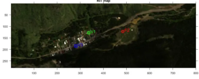
Fig. 1. Complete RGB view of the RIT test scene

The 800 × 280 pixel image (see Fig. 1), composed of N = 126 bands was collected in 2006, around the small town of Cooke City, Montana, USA. The data were obtained by the HyMap sensor on-board a plane flying at about 1.4 km altitude, resulting in a terrain resolution of about 3 × 3 meters. 4 kinds of fabric panels and 3 kinds of civilian cars were used as targets in this map. For each target, a reference spectrum signature obtained from a laboratory spectrophotometer is provided. Moreover, the targets’ map positions are also given for the self test (see Fig. 1). It should be noted that the spatial resolution of the map is of the same order of magnitude as the target sizes, so that they will usually behave as subpixel targets [23], [33].

From the three cars proposed as targets, we have chosen to

consider only the so-called V1 and V3 [21], as vehicle V2 is

a pick-up composed of two different signatures, namely the one corresponding to the cabin and the one corresponding to the back. Besides these two vehicles, a third detection

experiment will be conducted on the so-called F2 target,

corresponding to a 3 × 3 meter yellow nylon fabric panel.

The F1 panel being easily detectable, it is not discriminant

for our benchmark so that we have chosen not to consider

it. Moreover, panels F3 and F4 being multiple targets with

different sizes, are difficult to take into account in a simple detection scoring.

The mean and the covariance matrix of the background are

both estimated from an identical window whose size varies from 15 × 15 pixels, corresponding to the smallest number of secondary pixel to get an invertible covariance matrix, to the complete map, as specified in table I. It should be noted that some authors recommend using a shorter window to estimate the background mean, as this last vector is supposed to change more rapidly than the covariance matrix [34]. But, as the algorithms considered in this paper have been derived considering the same number of secondary data, both for the mean and the covariance matrix, we chose to use a unique window size. Moreover, given the size of the targets, we consider a 5 × 5 pixel guard window around the PUT, corresponding to 15 × 15 ground meters, to exclude the signature of a possible target in the background estimation process.

The performance of each benchmarked algorithm is assessed calculating the number of pixels having their detector’s output strictly higher than the one for the target pixel. This number can be seen as a false alarm number with an optimal thresholding. The proposed ACUTE scheme is compared with standard Gaussian detectors, namely the MF, Kelly’s detector, ACE, and the FTMF which is the only one also designed for the replacement model. We have also added the EC-FTMF for comparison, as it is a rare example of a detector exploiting the replacement model, even if it assumes a non-Gaussian background. In order to differentiate EC-FTMF from FTMF, we chose a small number of degrees of freedom for the assumed Student background probability density function (pdf) (ν = 3). The false alarm scores, calculated as described above are presented in Tables II, III and IV, for the 3 different targets, and for different secondary data window sizes. Moreover, the results for the global version of each detector, i.e. considering all the pixels as secondary data, is also included in the tables.

TABLE I

COVARIANCE WINDOW SIZES AND THE CORRESPONDING RELATIVE NUMBER OF SECONDARY PIXELS

Window Size 15 17 19 21 23 25 Global

K

N 1.71 2.22 2.8 3.43 4.13 4.89 1778

TABLE II

FALSEALARMSRITSCORE FORV1TARGET K

N MF Kelly ACE FTMF ECFTMF ACUTE

1778 399 398 16 32 15 32 4.89 253 70 19 117 14 33 4.13 196 39 8 84 6 23 3.43 188 30 9 86 8 19 2.8 337 50 33 154 25 33 2.22 183 10 8 90 6 9 1.71 74 1 1 37 1 1

First of all we can see that the False Alarm scores are very different for the 3 kinds of target, while they are approximately

of the same size. Thus we can expect that V3 probably gets

a spectral signature closer to background components. The ability of a given detector to mitigate the false alarms due to

(7)

TABLE III

FALSEALARMSRITSCORE FORV3TARGET K

1778 9635 9633 3848 3653 1663 3652 4.89 22695 16710 7766 10605 3792 7891 4.13 12107 7255 3448 5765 1698 3489 3.43 16938 9833 6000 8212 2907 4786 2.8 7956 3754 3047 3907 1471 1870 2.22 1409 112 65 726 35 64 1.71 4086 923 922 2042 441 468 TABLE IV

FALSEALARMSRITSCORE FORF2TARGET K

1778 0 0 3 0 3 0 4.89 0 0 0 0 0 0 4.13 0 0 0 0 0 0 3.43 1 0 0 0 0 0 2.8 1 0 0 0 0 0 2.22 1 0 0 0 0 0 1.71 4 1 1 1 1 1

target-like background is referred to as selectivity. The replace-ment model-based detectors are known to increase selectivity, as they cross-check the target fill factor and the background attenuation in the PUT. This selectivity improvement was in fact the starting point for the development of the replacement model-based FTMF [17]. On the other hand, the one-step approaches (Kelly, ACE and ACUTE) seem to be more robust to a small number of secondary pixels, as can be observed in the last two cells of tables II and III, where they belong to the best methods. We can notice a very good performance from the EC-FTMF, but it is difficult to draw any conclusions as it is the only one assuming a fat tail background distribution. The proposed detector ACUTE possesses the two features: it is a one-step approach and it is based on the replacement model. Thus it behaves all the better as the secondary window size decreases and if selectivity issues exist in the map. This can be observed in Table III, even if we can notice a very good performance from ACE too.

B. Viareggio Experiment

The second experiment we have chosen is the airborne Viareggio 2013 trial [22], as we have access here to the raw data. This way, we can control the pre-processing steps. Moreover, the spatial resolution of the map is thinner than for the RIT experiment, leading to more full-pixel targets and larger target abundances. This benchmarking hyperspectral detection campaign took place in Viareggio (Italy), in May 2013, where an aircraft flying at 1200 meters, acquired 3 [450 × 375] pixels maps of the same area. Two of them correspond to a cloudy day, whereas the last one was acquired during clear weather. Each pixel is composed of 511 samples in the Visible Near InfraRed (VINR) band (400 − 1000nm). The spatial resolution is about 0.6 meters.

Different kinds of vehicles as well as coloured panels served as known targets. For each of these targets, a spectral signature obtained from ground spectroradiometer measurements is available as well as the ground truth position. Moreover, a

black and a white cover, serving as calibration targets, were also deployed. Indeed, these two calibrated targets, can be used to convert the raw Digital Numbers (DN) measurements into a reflectance map, using for instance the Empirical Line Method (ELM) [35] [36].

Fig. 2. Complete RGB view of the D1F12H1 Viareggio test scene

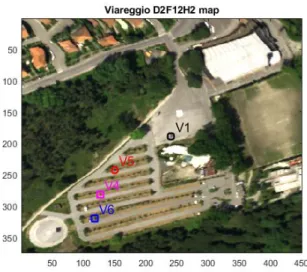
Fig. 3. Complete RGB view of the D1F12H2 Viareggio test scene The 3 experiments have been conducted with different target configurations, as represented in Figs. 2, 3 and 4. The scene is composed of parking lots, roads, buildings, sport fields and pine woods. The black and white calibration panels are clearly visible, around positions [70, 330] and [250, 150] respectively. Moreover, the targets are composed of 5 vehicles (mentioned with a V) and 1 panel (mentioned with a P). As for the RIT

experiment, we have excluded the so-called P1 panel as it is

composed of 3 distinct pieces.

The first step of the processing aims at converting the raw measurements into a reflectance map, for which the unitary constraint on the abundances is supposed to be verified. To this end, we use the ELM, considering the black and white

(8)

Fig. 4. Complete RGB view of the D2F12H2 Viareggio test scene

calibration panels. Then spectral binning [37] is performed to reduce the vector size dimension to N = 32.

Tables VI- XVII present the false alarm scores, computed as for the RIT experiment, for the different detectors, for the different targets, the different maps and different window sizes. For this benchmark, we have chosen a guard window size of 9×9 pixels, in order to avoid the presence of target signature in the covariance matrix estimation window. The correspondence between the covariance window sizes and the relative number

of secondary pixels, namely _Nk is presented in table V.

TABLE V

COVARIANCE WINDOW SIZES AND THE CORRESPONDING RELATIVE NUMBER OF SECONDARY PIXELS

Window Size 11 13 15 17 19 21 Global

K

N 1.25 2.72 4.5 6.5 8.75 11.2 5271

TABLE VI

FALSEALARMS SCORE FORV1TARGET IN THED1F 12H1 VIAREGGIO OPEN DATA IMAGE

K

5271 3 3 3 2 1 2 11.2 0 0 0 0 0 0 8.75 0 0 0 0 0 0 6.5 0 0 0 0 0 0 4.5 0 0 0 0 0 0 2.75 1 0 0 0 0 0 1.25 19 9 11 8 5 4

As for the RIT experiment, we can observe a good perfor-mance of the proposed ACUTE especially for small window

sizes, except for the V3 target on the two first images and

the V6 on the last map. Indeed, for these 2 specific targets

we encounter a performance loss with respect to the other targets, especially when the window size increases. In our experience this loss can be mitigated using a covariance matrix regularization scheme. Indeed, we experienced that diagonal loading of the sample covariance matrix before inversion can largely improve the performances compared to the other

TABLE VII

K

5271 26 26 1 133 1 133 11.2 68 45 49 700 21 454 8.75 68 41 38 801 43 467 6.5 79 54 71 1108 35 677 4.5 110 108 239 2089 70 1003 2.75 143 158 235 2530 78 527 1.25 139 183 289 522 241 489 TABLE VIII

K

5271 0 0 0 0 0 0 11.2 0 0 2 0 0 0 8.75 0 0 2 0 0 0 6.5 0 0 2 0 0 0 4.5 0 0 0 0 0 0 2.75 1 0 0 0 0 0 1.25 3 6 19 0 1 1 TABLE IX

FALSEALARMS SCORE FORP2TARGET IN THED1F 12H1 VIAREGGIO OPEN DATA IMAGE

K

5271 2 2 0 0 0 0 11.2 4 7 10 1 0 1 8.75 7 8 15 6 0 3 6.5 8 9 16 5 0 1 4.5 9 16 24 2 0 2 2.75 9 11 25 4 0 1 1.25 10 18 13 4 3 3 TABLE X

K

5271 0 0 1 0 2 0 11.2 12 1 8 3 0 0 8.75 13 2 11 5 0 0 6.5 13 3 12 10 1 1 4.5 14 4 27 15 2 3 2.75 17 6 21 23 3 3 1.25 5070 4105 4225 2914 1479 1538 TABLE XI

K

5271 16 16 1 94 5 94 11.2 58 47 79 201 8 119 8.75 39 40 58 250 18 110 6.5 60 47 65 275 33 101 4.5 73 45 76 429 30 126 2.75 219 303 823 1196 21 139 1.25 9684 7391 6297 6401 2323 2507

detectors. This issue is beyond the scope of the present paper and will be investigated in future work. Once again, we observe very good performance of the EC-FTMF algorithm, suggesting a better fit of a fat-tail pdf for the background than

(9)

TABLE XII

K

5271 0 0 1 1 1 1 11.2 0 0 6 0 0 0 8.75 0 1 6 0 0 0 6.5 0 0 6 0 0 0 4.5 0 1 4 0 0 0 2.75 0 0 0 0 0 0 1.25 4411 2925 2920 1198 1289 1318 TABLE XIII

FALSEALARMS SCORE FORP2TARGET IN THED1F 12H2 VIAREGGIO OPEN DATA IMAGE

K

5271 0 0 0 0 0 0 11.2 3 6 11 10 0 6 8.75 6 6 17 11 0 4 6.5 3 6 17 14 0 6 4.5 2 1 4 14 0 4 2.75 2 2 3 5 0 1 1.25 5291 5475 5909 2253 1635 1763 TABLE XIV

K

5271 1 1 3 1 2 1 11.2 0 0 0 0 0 0 8.75 0 0 0 0 0 0 6.5 0 0 0 0 0 0 4.5 0 0 0 0 0 0 2.75 0 0 0 0 0 0 1.25 2471 1392 1400 798 760 776 TABLE XV

K

5271 0 0 0 1 0 1 11.2 0 0 0 0 0 0 8.75 0 0 0 0 0 0 6.5 0 0 0 0 0 0 4.5 0 0 0 0 0 0 2.75 0 0 0 0 0 0 1.25 2529 1406 1412 720 728 747 TABLE XVI

K

5271 0 0 0 0 0 0 11.2 0 0 0 0 0 0 8.75 0 0 0 0 0 0 6.5 1 0 0 0 0 0 4.5 7 0 0 1 0 0 2.75 8 0 0 2 0 0 1.25 2859 1535 1487 1126 773 807 a Gaussian one.

Figure 5 presents the detector outputs for the P2 target and

for a 100×100 pixel zoom around the target. These plots show the enhanced selectivity of the two replacement model based

TABLE XVII

K

5271 42 42 3 1205 0 1205 11.2 151 102 25 75 20 70 8.75 142 99 17 110 9 84 6.5 109 93 28 216 1 163 4.5 147 95 55 284 1 133 2.75 104 97 86 7 1 2 1.25 3598 3200 3543 1101 815 843 Area of Interest 20 40 60 80 100 20 40 60 80 100 0 0.2 0.4 0.6 0.8 1 MF 20 40 60 80 100 20 40 60 80 100 200 400 600 800 1000 1200 Kelly 20 40 60 80 100 20 40 60 80 100 10 20 30 40 50 60 ACE 20 40 60 80 100 20 40 60 80 100 0.1 0.2 0.3 0.4 0.5 0.6 0.7 FTMF 20 40 60 80 100 20 40 60 80 100 0 50 100 150 ACUTE 20 40 60 80 100 20 40 60 80 100 0 5 10 15 20 25 30

Fig. 5. Outputs of the detectors for P2 target

detectors, namely FTMF and ACUTE. Indeed, for the three other detectors, in addition to the target peak in the center of the plots, we can clearly see many interference peaks corre-sponding to the parking-lot splitters that can be seen in the top left figure. As stated before, while the detectors designed for the additive model only measure the matching between the PUT and the target signature, after background whitening, FTMF and ACUTE also check the correspondence between the target abundance, α and the background attenuation. If the background attenuation does not correspond to (1 − α), their output should decrease.

To finish with, we have also plotted the estimated target abundance α both for the FTMF and ACUTE, in figure 6. In both cases, we see a maximum value in the center of the map, corresponding to the target position. The target abundance are respectively estimated at 0.45 and 0.59 for FTMF and ACUTE. These results are smaller than the supposed target fill factor, which should be 1 in the center of the map where only the target is present (full-pixel target). This under-estimation is probably due to mismatches between the real target signature and the presumed one, as well as the representativity of the

(10)

α FTMF 20 40 60 80 100 20 40 60 80 100 0 0.1 0.2 0.3 0.4 α acute 20 40 60 80 100 20 40 60 80 100 0 0.1 0.2 0.3 0.4 0.5

Fig. 6. ˆα for FTMF and ACUTE

mean and covariance matrix estimated from the secondary data.

C. Statistical Experiment

As stated before, we now conduct a statistical experiment in this last subsection. To this end, we consider the Viareggio first image and insert a target that is not initially present

in the map. More precisely, we insert the target V5 or V6,

only present in the third Viareggio map, according to the replacement model with two specific values of the fill factor α = 0.2 and α = 0.05. This last value corresponds to a case where the replacement model tends towards the additive one. For each Monte-Carlo trial the position of the target is randomly changed and the detector output for the pixel of

interest is recorded to estimate the probability of detection Pd.

The total image without target serves as reference to compute

the probability of false alarm Pf a. Changing the threshold

position, we can plot the receivers operation characteristics

(ROC) as represented on Figs. (7) and (8) for V5 and Figs.

(9) and (10) for V6, for a secondary window size of 13 × 13.

This size corresponds to 5 more secondary pixels than the vector size N . Moving to larger windows does not change significantly the results presented hereafter.

10-6 10-5 10-4 10-3 10-2 10-1 100 Pfa 0 0.1 0.2 0.3 0.4 0.5 0.6 0.7 0.8 0.9 1 Pd

Simulated targets with V

5 signature, on Viareggio image, = 0.2

AMF Kelly ACE FTMF ECFTMF ACUTE

Fig. 7. Receivers operation characteristics for V5 with α = 0.2

We can see that the gain using replacement-based algo-rithms, namely FTMF or ACUTE, can reach two decades

in terms of Pf a for a given Pd, as soon as α reaches 0.2.

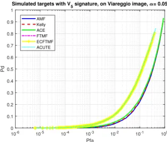
10-6 10-5 10-4 10-3 10-2 10-1 100 Pfa 0 0.1 0.2 0.3 0.4 0.5 0.6 0.7 0.8 0.9 1 Pd

Simulated targets with V₅ signature, on Viareggio image, = 0.05

Fig. 8. Receivers operation characteristics for V5with α = 0.05

10-6 10-5 10-4 10-3 10-2 10-1 100 Pfa 0 0.1 0.2 0.3 0.4 0.5 0.6 0.7 0.8 0.9 1 Pd

Simulated targets with V₆ signature, on Viareggio image, = 0.2

Fig. 9. Receivers operation characteristics for V6with α = 0.2

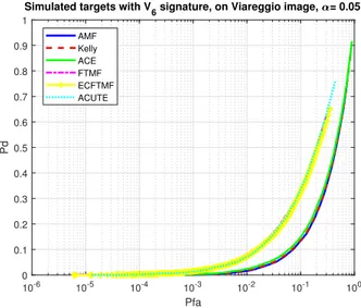
This improvement is higher than that observed in the real data experiment, possibly because here the data have been generated considering the exact replacement model. Thus, the

two algorithms perfectly match the signal under H1, unlike in

the real data cases, where the data follow, most probably, a more complicated model, including possible non-linearities or other mismatches.

To finish with, we compare the estimated values of the fill factor α given by FTMF, ACUTE and EC-FTMF. Fig. 11 represents the histograms of the 10000 Monte-Carlo trials for

the V6 target with α = 0.2. We can see a good accordance

between the estimated values and the real one for both the 3 algorithms, even if the FTMF and EC-FTMF slightly under-estimate the actual value of α of 10% in average, unlike for the ACUTE procedure, which seems to be unbiased.

VI. CONCLUSIONS

In this paper we considered the detection problem of a subpixel target in an hyperspectral image. The observations

(11)

10-6 10-5 10-4 10-3 10-2 10-1 100 Pfa 0 0.1 0.2 0.3 0.4 0.5 0.6 0.7 0.8 0.9 1 Pd

Simulated targets with V₆ signature, on Viareggio image, = 0.05

Fig. 10. Receivers operation characteristics for V6 with α = 0.05

Fig. 11. Histograms of estimated α for V6with α = 0.2 and 13×13 window

are assumed to follow the so-called replacement model, driven by the constraint of a unitary sum for the abundances. While the most frequently used algorithms have been developed for the approximated additive model, very few procedures rely on the replacement model. As a completion of the detectors for Gaussian distributions, we derive the direct GLRT, which is the counterpart of the popular Kelly’s detector, for the replacement model case. This detector is shown to rank among the very best popular algorithms, on real data benchmarking, especially for small secondary data windows, and when selectivity issues can occur in the map.

REFERENCES

[1] D. G. Manolakis, R. B. Lockwood, and T. W. Cooley, Hyperspectral Imaging Remote Sensing. Cambridge University Press, 2016. [2] E. Keith, H. Dan, O. William, J. Shridhar, B. Eustace, and L. Dereniak,

“Hyperspectral imaging for astronomy and space surveillance,” in Proc. SPIE, vol. 5159, January 2004.

[3] S. Michel, P. Gamet, and M.-J. Lefevre-Fonollosa, “Hypxim — a hyperspectral satellite defined for science, security and defence users,” in Proceesings 3rd Workshop on Hyperspectral Image and Signal Processing: Evolution in Remote Sensing (WHISPERS), June 2011.

[4] H. Kwon and N. Nasrabadi, “Kernel rx-algorithm: a nonlinear anomaly detector for hyperspectral imagery,” IEEE Transactions Geoscience Remote Sensing, vol. 43, no. 2, pp. 388–397, January 2005.

[5] E. M. Winter, M. Miller, C. Simi, A. Hill, T. Williams, D. Hampton, M. Wood, J. Zadnick, and M. Sviland, “Mine detection experiments using hyperspectral sensors,” in SPIE Int. Soc. Opt. Eng., Orlando, FL, United States, 21 September 2004.

[6] C. C. Funk, J. Theiler, D. A. Roberts, and C. C. Borel, “Clustering to improve matched filter detection of weak gas plumes in hyperspec-tral thermal imagery,” IEEE Transactions Geoscience Remote Sensing, vol. 39, no. 7, pp. 1410–1420, July 2001.

[7] D.-W. Sun, Hyperspectral Imaging for Food Quality Analysis and Control. Elsevier, 2010.

[8] R. Koprowski, Processing of Hyperspectral Medical Images, Applica-tions in Dermatology Using Matlab . Springer International Publish-R

ing, 2017.

[9] N. Dobigeon, J.-Y. Tourneret, C. Richard, J. C. M. Bermudez, S. McLaughlin, and A. O. Hero, “Nonlinear unmixing of hyperspectral images,” IEEE Signal Processing Magazine, pp. 82–94, January 2014. [10] E. Kelly, “An adaptive detection algorithm,” IEEE Transactions

Aerospace Electronic Systems, vol. 22, no. 2, pp. 115–127, March 1986. [11] F. C. Robey, D. R. Fuhrmann, E. J. Kelly, and R. Nitzberg, “A CFAR adaptive matched filter detector,” IEEE Transactions Aerospace Electronic Systems, vol. 28, no. 1, pp. 208–216, January 1992. [12] S. Kraut, L. L. Scharf, and L. T. McWhorter, “Adaptive subspace

detectors,” IEEE Transactions Signal Processing, vol. 49, no. 1, pp. 1–16, January 2001.

[13] D. Manolakis and G. Shaw, “Detection algorithms for hyperspectral imaging applications,” IEEE Signal Processing Magazine, pp. 29–43, January 2002.

[14] J. Settle, “On constrained energy minimization and the partial unmixing of multispectral images,” IEEE Transactions Geoscience Remote Sens-ing, vol. 40, no. 3, pp. 718–721, March 2002.

[15] C. Chang, “Orthogonal subspace projection (osp) revisited: A com-prehensive study and analysis,” IEEE Transactions Geoscience Remote Sensing, vol. 43, no. 3, pp. 502–518, March 2005.

[16] J. Theiler and B. R. Foy, “EC-GLRT: Detecting weak plumes in non-Gaussian hyperspectral clutter using an elliptically-contoured general-ized likelihood ratio test,” in Proceedings IGARSS, vol. 1, Boston, MA, July 2008, pp. 221–224.

[17] A. Schaum and A. Stocker, “Spectrally-selective target detection,” in Proceedings of ISSSR, vol. 12, April 1997, pp. 2015–2018.

[18] J. Theiler, B. Zimmer, and A. K. Ziemann, “Closed-form detector for solid sub-pixel targets in multivariate t-distributed background clutter,” in Proceedings IGARSS, Valencia, Spain, July 2018, pp. 2773–2776. [19] D. Manolakis, R. Lockwood, T. Cooley, and J. Jacobson, “Is there a best

hyperspectral detection algorithm?” in Proc. of SPIE, vol. 7334, 2009. [20] F. Vincent, O. Besson, and C. Richard, “Matched subspace detection

with hypothesis dependant noise power,” IEEE Transactions Signal Processing, vol. 56, no. 11, pp. 5713–5718, November 2008. [21] D. Snyder, J. Kerekes, I. Fairweather, R. Crabtree, J. Shive, and S. Hager,

“Development of a web-based application to evaluate target finding algorithms,” in in Geoscience and Remote Sensing Symposium, 2008. IGARSS 2008, vol. 2, 2008, pp. II–915.

[22] N. Acito, S. Matteoli, A. Rossi, M. Diani, and G. Corsini, “Hyperspectral airborne “viareggio 2013 trial” data collection for detection algorithm assessment,” IEEE Journal of Selected Topics in Applied Earth Obser-vations and Remote Sensing, vol. 9, no. 6, pp. 2356–2376, June 2016. [23] V. Roy, “Hybrid algorithm for hyperspectral target detection,” in Proc.

SPIE 7695, Algorithms and Technologies for Multispectral, Hyperspec-tral, and Ultraspectral Imagery XVI, 769522, May 2010.

[24] J. P. Kerekes and D. K. Snyder, “Unresolved target detection blind test project overview,” in Proc. SPIE 7695, Algorithms and Technologies for Multispectral, Hyperspectral, and Ultraspectral Imagery XVI, 769521, vol. 7695, May 2010.

[25] B. H. Gang Wang, Ying Zhang and K. T. Chong, “A framework of target detection in hyperspectral imagery based on blind source extraction,” IEEE Journal of Selected Topics in Applied Earth Observations and Remote Sensing, vol. 9, no. 2, pp. 835–844, FEBRUARY 2016. [26] M. S. Halper, “Global, local, and stochastic background modeling for

target detection in mixed pixels,” in Proc. SPIE 7695, Algorithms and Technologies for Multispectral, Hyperspectral, and Ultraspectral Imagery XVI, 769527, vol. 7695, May 2010.

[27] Y. Cohen, Y. August, D. G. Blumberg, and S. R. Rotman, “Evaluating subpixel target detection algorithms in hyperspectral imagery,” Journal of Electrical and Computer Engineering - Hindawi, vol. 2012, 2012.

(12)

[28] S. Yang and Z. Shi, “SparseCEM and sparseACE for hyperspectral image target detection,” IEEE Geoscience and Remote Sensing Letters, vol. 11, no. 12, pp. 2135–2139, Dec 2014.

[29] S. Yang, Z. Shi, and W. Tang, “Robust hyperspectral image target detec-tion using an inequality constraint,” IEEE Transacdetec-tions on Geoscience and Remote Sensing, vol. 53, no. 6, pp. 3389–3404, June 2015. [30] Y. Liang, P. P. Markopoulos, and E. S. Saber, “Subpixel target detection

in hyperspectral images with local matched filtering in slic superpixels,” in 8th IEEE Workshop on Hyperspectral Image and Signal Processing: Evolutions in Remote Sensing (WHISPERS 2016), August 2016. [31] L. Zhang, L. Zhang, D. Tao, X. Huang, and B. Du, “Hyperspectral

remote sensing image subpixel target detection based on supervised metric learning,” IEEE Transactions on Geoscience and Remote Sensing, vol. 52, no. 8, pp. 4955–4965, Aug 2014.

[32] E. J. Ientilucci, S. Matteoli, and J. P. Kerekes, “Tracking of vehicles across multiple radiance and reflectance hyperspectral datasets,” in Proc. SPIE 7334, Algorithms and Technologies for Multispectral, Hyperspec-tral, and Ultraspectral Imagery XV, 73340A, April 2009.

[33] S. Khazai, A. Safari, B. Mojaradi, and S. Homayouni, “An approach for subpixel anomaly detection in hyperspectral images,” IEEE IEEE Journal of Selected Topics in Applied Earth Observations and Remote Sensing, pp. 1–10, April 2013.

[34] S. Matteoli, M. Diani, and G. Corsini, “A tutorial overview of anomaly detection in hyperspectral i mages,” IEEE Aerospace Electronics Systems Magazine, vol. 25, no. 7, pp. 5–27, July 2010.

[35] G. Ferrier, “Evaluation of apparent surface reflectance estimation methodologies,” International Journal of Remote Sensing, vol. 16, pp. 2291–2297, 1995.

[36] G. M. Smith and E. J. Milton, “The use of the empirical line method to calibrate remotely sensed data to reflectance,” International Journal of Remote Sensing, vol. 20, pp. 2653–2662, 1999.

[37] M. Shi and G. Healey, “Hyperspectral texture recognition using a multi-scale opponent representation,” IEEE Transactions Geoscience Remote Sensing, vol. 41, no. 5, pp. 1090–1095, May 2003.