Ensemble-based data assimilation for operational flood forecasting – On the merits of state estimation for 1D hydrodynamic forecasting through the example of the “Adour Maritime” river

O

pen

A

rchive

T

OULOUSE

A

rchive

O

uverte (

OATAO

)

OATAO is an open access repository that collects the work of Toulouse researchers and

makes it freely available over the web where possible.

This is an author-deposited version published in :

http://oatao.univ-toulouse.fr/

Eprints ID : 19867

To link to this article : DOI:

10.1016/j.jhydrol.2017.06.017

URL

http://dx.doi.org/10.1016/j.jhydrol.2017.06.017

To cite this version : Barthélémy, Sébastien and Ricci, Sophie and

Rochoux, Mélanie C. and Le Pape, Etienne and Thual, Olivier:

Ensemble-based data assimilation for operational flood forecasting – On

the merits of state estimation for 1D hydrodynamic forecasting through

the example of the “Adour Maritime” river (2017), Journal of Hydrology,

vol. 552, pp. 210-224

Any correspondance concerning this service should be sent to the repository

administrator:

staff-oatao@listes-diff.inp-toulouse.fr

Research papers

Ensemble-based data assimilation for operational flood forecasting – On

the merits of state estimation for 1D hydrodynamic forecasting through

the example of the ‘‘Adour Maritime” river

S. Barthélémy

a,⇑

_{, S. Ricci}

a

_{, M.C. Rochoux}

a

_{, E. Le Pape}

b

_{, O. Thual}

a c, a

CECI, CNRS-CERFACS, Toulouse, France b_{SCHAPI, Toulouse, France}

c

IMFT, INPT, CNRS, Toulouse, France

a r t i c l e

i n f o

Keywords: Hydraulic modeling Flood forecasting Data assimilation Uncertainty reduction Ensemble approach

a b s t r a c t

This study presents the implementation and the merits of an Ensemble Kalman Filter (EnKF) algorithm with an inflation procedure on the 1D shallow water model MASCARET in the framework of operational flood forecasting on the ‘‘Adour Maritime” river (South West France). In situ water level observations are sequentially assimilated to correct both water level and discharge. The stochastic estimation of the back-ground error statistics is achieved over an ensemble of MASCARET integrations with perturbed hydrolog-ical boundary conditions. It is shown that the geometric characteristics of the network as well as the hydrological forcings and their temporal variability have a significant impact on the shape of the univari-ate (wunivari-ater level) and multivariunivari-ate (wunivari-ater level and discharge) background error covariance functions and thus on the EnKF analysis. The performance of the EnKF algorithm is examined for observing system sim-ulation experiments as well as for a set of eight real flood events (2009–2014). The quality of the ensem-ble is deemed satisfactory as long as the forecast lead time remains under the transfer time of the network, when perfect hydrological forcings are considered. Results demonstrate that the simulated hydraulic state variables can be improved over the entire network, even where no data are available, with a limited ensemble size and thus a computational cost compatible with operational constraints. The improvement in the water level Root-Mean-Square Error obtained with the EnKF reaches up to 88% at the analysis time and 40% at a 4-h forecast lead time compared to the standalone model.

1. Introduction

Flood and inundation represent major societal and economic issues (Guha-Sapir et al., 2012; Stocker et al., 2013; World Meteorological Organization, 2011). For instance, 2016 European floods caused a total loss of about 1 billion euros and 19 deaths. Anticipating and monitoring in real-time strong flood events is thus a key challenge for national and international flood forecast-ing agencies, which are in charge of water level and discharge pre-diction, risk assessment and alert system to inform government authorities and general public (Weerts et al., 2011;Werner et al., 2009). For this purpose, they rely on the complementary use of observations and numerical models. In France, the national flood forecasting center (SCHAPI – Service Central d’Hydrométéorologie

et d’Appui à la Prévision des Inondations) is since 2006, in charge of the surveillance of 22,000 km of rivers and provides, in collabo-ration with the 22 local flood forecasting services (SPC – Service de Prévision des Crues), producing a twice-daily color-scaled risk map available on-line1_.

Several sources of uncertainty have been identified in hydraulic models as barriers to forecast process improvement. On the one hand, input data to the model represent a substantial source of uncertainty. For instance, hydrological forcing data that describe boundary conditions for hydraulic models usually result from the transformation of uncertain observed water levels into discharges through an uncertain rating curve (Audinet and André, 1995), or from discharges that are forecast by uncertain hydrological mod-els. On the other hand, the simplification of the flow to a 1D repre-sentation (with or without flood plain description) is a significant

sentation (with or without flood plain description) is a significant limitation. Model equations are based on physics simplification

⇑Corresponding author at: 42 Avenue Gaspard Coriolis, 31057 Toulouse Cedex 01, France.

and parametrization. These parametrization schemes are cali-brated to adjust the model behavior to observed water levels, typ-ically through the calibration of friction coefficients that is a pragmatic way to account for various sources of uncertainty. Uncertainties in the input data and in the hydraulic parameters translate into uncertainties in the simulated hydraulic state. Many studies intent to quantify and account for uncertainties in hydro-logical and hydraulic models (Vrugt et al., 2008; Bozzi et al., 2014). Estimating the model output probability density function (PDF) induces a significant computational cost. In the present work, the focus is made on a data assimilation (DA) method that relies on estimating the first two statistical moments, the mean and the standard deviation (STD) of the hydraulic state, instead of its complete PDF to be compatible with operational framework. In order to overcome the limitations of both hydraulic models and observations, DA combines information from the numerical model with observations along with modeling and observational errors, thus reducing the range of uncertainty in the model out-puts. While originating from meteorology and oceanography, DA has been recently successfully applied to hydrodynamics (Madsen and Skotner, 2005; Biancamaria et al., 2011; Ricci et al., 2011). Filtering methods have been widely applied for hydraulic DA as the cost of the numerical model and the size of the state vec-tor remain limited. For instance,Jean-Baptiste et al. (2011) esti-mated ungauged lateral forcings on the Rhône river, South East France, with a Kalman Filter (KF) and a particle filter through an extended control vector adding unknown forcings to the state vec-tor. Ricci et al. (2011) estimated in a two-step procedure the upstream forcings on the Adour river, South West France, with an extended Kalman Filter thus accounting for model nonlineari-ties and featuring an invariant forecast error covariance matrix (IKF). Similarly to work achieved byMadsen and Skotner (2005) and Shiiba et al. (2000), a stationary description of the KF back-ground error covariance matrix was used in order to lower the algorithm computational cost, with asymmetric functions charac-terized by a larger correlation length scale upstream than down-stream of the observing stations. These statistics do not take into account flow dependency nor river geometry dependency (slope or river width variation). The IKF algorithm was able to correct the hydraulic state (water level and discharge) and to significantly improve the forecast up to 12-h lead time. Following this work,

Habert et al. (2016)extended the IKF algorithm to the estimation of the friction coefficients using in situ water level measurements, thus improving the model water-level/discharge relationship and the flood phase. Studies have also explored the use of the Ensemble Kalman Filter (EnKF) that is believed to bring insightful informa-tion on the background error covariance funcinforma-tions and their flow non-static dependence. The EnKF (Evensen, 1994) stochastically estimates them over an ensemble of members, i.e. a sample of model integrations that represents the uncertainty in the model state.Hartnack et al. (2005)used the EnKF to assimilate water level and discharge in a 1D-2D flood model, thus improving both hydraulic state and forcings. Several studies demonstrated the benefits of the EnKF assimilating satellite observations (Andreadis et al., 2007; Biancamaria et al., 2011; Durand et al., 2008; Giustarini et al., 2011; Matgen et al., 2010; Neal et al., 2009; Yoon et al., 2012). For instance,Durand et al. (2008)showed that the EnKF is successful at rebuilding river bathymetry through the assimilation of synthetic remote sensing data.

The objective of the paper is to demonstrate, in both analysis and forecast modes, the merits of a state estimation EnKF algo-rithm on the 1D shallow water model MASCARET in the framework

that the use of Desroziers’ criteriaDesroziers et al. (2005) com-bined with a specific methodology presented in Miyoshi (2005)

and applied in Li et al. (2009)allows for a proper estimation of the observation error statistics. The stochastic estimation of the background error statistics is achieved over an ensemble of MAS-CARET integrations with perturbed hydrological boundary condi-tions. Assuming that errors in simulated water level are mostly due to uncertainty in forcing input data is a common hypothesis (Maggioni et al., 2012; Alemohammad et al., 2015; Dumedah and Walker, 2017; Li et al., 2016). Perturbed hydrological forcing fields are generated assuming that the hydrological forcing field error is a time-varying Gaussian Process with a Gaussian correlation func-tion of fixed length scale. The novelty in the present paper is that the explicit formulation of background error covariances with EnKF allows for time and space description of background error statis-tics. An inflation method is implemented combining work from

Anderson (2007) and Li et al. (2009), in order to enlarge the spread of uncertainty within the ensemble, which tends to be under-dispersive in forecast mode. The resulting algorithm is denoted by IEnKF (Inflated Ensemble Kalman Filter). The merits of the IEnKF for reducing uncertainty is shown on water level and discharge ensemble simulations and means over synthetic experiments rep-resentative of flood conditions (Observing System Simulation Experiments – OSSE) as well as the re-analysis of eight recent flood events (2009–2014) on the ‘‘Adour Maritime” network.

The structure of the paper is as follows: Section2provides a description of MASCARET and the ‘‘Adour Maritime” river. The IEnKF is presented in Section3with focus on ensemble generation, a posteriori observation error estimation, inflation, numerical implementation and performance metrics. DA results are detailed in Section . Conclusions and perspectives for this work are given4

in Section .5

2. Modeling of the Adour river 2.1. The 1D hydraulic model MASCARET

MASCARET2_{is a component of the open-source integrated suite}

of solvers TELEMAC-MASCARET for use in the field of free surface flow modeling and is mainly developed by EDF and CEREMA (Goutal and Maurel, 2002). It solves the following conservative form of the 1D shallow water equations:

@S @tþ @Q @x¼ qa @Q @tþ @ @x Q2 S   þ gS@Z @x¼ gSSf; 8 < :

where is the wetted area (mS 2_{),Qis the discharge (m}3_s1_{), q} ais the lateral inflow (m2_s1_{),gstands for the gravity (m s}2_{), Zs is the free} surface height (m) and Sf is the friction modeled with the Strickler formula: Sf ¼ Q

2

K2 sS2R4 3h=

, with Ksthe Strickler coefficient (m1/3s1) and Rh(m) the hydraulic radius. In this work, we use the unsteady ker-nel of MASCARET based on the well-balanced finite volume Roe scheme (Roe, 1981) developed byGoutal and Maurel (2002). From MASCARET outputs can be derived the water level (or water height) of the free surface (m). The pair (Z Z Q; ) is referred to as the hydrau-lic state in the following.

The practical implementation of the ‘‘Adour Maritime” hydrau-lic model requires the following input data: bathymetry, upstream and downstream boundary conditions, lateral inflows, roughness coefficients and initial condition for the hydraulic state. The

imper-rithm on the 1D shallow water model MASCARET in the framework of operational flood forecasting on the ‘‘Adour Maritime” river in South West France. In situ water level observations are sequen-tially assimilated to correct both water level and discharge (space borne data are not yet used at operational level). It is first shown

coefficients and initial condition for the hydraulic state. The imper-fect description of these data translate into errors in the simulated water state.

2.2. The Adour river

The ‘‘Adour Maritime” hydraulic network (Fig. 1) is located in South West France, close to the Atlantic Ocean. The 161-km long section of the river network used in this work is composed of 7 reaches with 3 confluences and 3 dams located on reaches 3, 6 and 7. The entire network is under tidal influence except upstream of the dams.

The tidal influence of the Atlantic Ocean combined with the influence of the Pyrenees mountainous region result in a complex atmospheric and hydraulic dynamic over the Adour catchment. According to SCHAPI’s statistical records, the Adour catchment is ranked amongst the most challenging catchments in France due to a large number of severe alerts annually (orange and red levels on the color-scaled risk map produced by SCHAPI). The alerts are defined by water level thresholds at Cambo, Orthez, Dax, Escos and Peyrehorade. For example, the yellow, orange and red thresh-olds at Peyrehorade are set to 2.1, 4.1 and 4.9 m, respectively. Flood events can be categorized in three types. First, flood peaks occur-ring on reach 4 with a slow dynamic over 7 to 14 days and maxi-mum discharge between 400 and 1000 m3_s1_{. Second, flood} peaks on reaches 6 and 7 resulting from flash flood events over 2 to 3 days with a maximum discharge between 800 and 1650 m3_s1_{for reach 6 and a maximum discharge between 400} and 1100 m3_s1

for reach 7. Third, flood peaks on reach 3 that are eventually correlated in time with flood peaks on reaches 6 and 7 and last 2 to 3 days. These events might occur simultane-ously and be worsened by tidal influence.

In this context, upstream forcings are described by observed water levels (available at 15-min rate) translated into discharges with a local rating curve established at the observing stations of Dax, Orthez, Escos and Cambo. Since rating curves are built from a limited number of measurements and are usually extrapolated for higher flows, there are significant uncertainties due to these upstream boundary conditions. The downstream forcing is given by observed water level at the observing station of Convergent on the Atlantic Ocean’s coast. Water level observations are avail-able hourly at Peyrehorade, Urt, Villefranque, Pont-Blanc and

Lesseps. It takes approximately 5, 10 and 12 h for the upstream forcings to propagate to Peyrehorade and Pont-Blanc, Urt and Les-seps, respectively. In forecast simulation mode, the upstream hydrological forcings are set constant to the last observed value beyond this transfer time, and the downstream forcing is given by the forecast water level computed by the French national hydrographic and oceanographic service SHOM (Service Hydro-graphique et OcéanoHydro-graphique de la Marine).

The 1D hydraulic model terrain is described with 548 topo-graphic and bathymetric cross sections interpolated over 2795 grid points. The river is represented as a 1D flow bounded with infinite banks except in the neighboring of Peyrehorade, where a limited number of cross sections gives a local description of the flood plains. This model was developed for operational purposes by the Gironde-Adour-Dordogne (GAD) SPC in collaboration with SCHAPI. It suffers from three major limitations. First, some lateral inflows are not accounted for in the hydraulic model resulting in incorrect simulated water level during major flood events. Second, the mod-eling of the network with infinite banks and then the lack of flood plains on most of the domain result in errors when the simulated water level rises above the banks height. Third, errors in rating curves at observing stations may lead to the use of wrong dis-charge values for friction calibration. Nonetheless, sensitivity anal-ysis of the simulated water level according to the friction coefficient in the vicinity of Urt and Peyrohorade show that the simulated water level error are not completely due to the friction coefficient error, especially at the flood peak. We assume each fric-tion coefficient follows a Gaussian distribufric-tion centered around the calibrated value with a variance of 16.Fig. 2shows the water level PDF at Peyrehorade resulting from a Monte Carlo sampling (5000 members) of the friction coefficient Ksat Peyrehorade. The resulting water level PDF obtained with MASCARET (black line) features a 5-cm STD and slightly deviates from the Gaussian fit (red line). Similar results (not show here) are obtained for down-stream and updown-stream friction areas. The water level error explained by friction errors is thus significantly smaller than the differences between the free run and the observation that are observed at flood peak in this study (up to 1 m at Peyrehorade

Fig. 1. Hydraulic network scheme of the ‘‘Adour Maritime” river network simulated with MASCARET with reach indices. Water level observing stations are represented by red crosses. Dams on reaches 3, 6 and 7 are represented by black markers.

and 50 cm at Urt, seeFig. 16). The most significant errors for this hydraulic model are most likely due to upstream/lateral forcings and the incomplete river geometry description. Independently of the sources of the errors, the DA algorithm targets here the water level.

3. Ensemble-based data assimilation algorithm 3.1. Ensemble-based state estimation approach

The EnKF algorithm (Evensen, 1994) implemented in this work solves a state estimation problem. The control vector denoted by x is composed of the hydraulic state, i.e. the discretized water level and discharge over space. The EnKF decomposes in an analysis step and a forecast step that are sequentially applied to correct the hydraulic statex(Fig. 3presents a schematic of the assimilation cycle½ i 1; iwith the EnKF analysis achieved at time ). The EnKFi relies on the MASCARET integration of an ensemble of Neperturbed members xb k;

i (indexed by the superscript bstanding for ‘‘back-ground”) and on the assumption that the stochastic estimate of the ensemble statistics is a fair representation of the model state

error statistics. For an analysis at time , the background errori covariance matrix Biis stochastically estimated as:

Bi ¼ 1 Ne 1 XNe k¼1 xb k; i  x b i   xb k; i  x b i  T ; ð Þ1

where k corresponds to the index of the ensemble member, xb

i ¼N1e

PNe

k¼1x b k;

i corresponds to the ensemble mean over the back-ground members andTstands for the transposition operator. Then, the Kalman gain Ki is computed with Ki¼ BiHT HBiHTþ R

 1 , whereHis the tangent linear of the observation operatorHthat maps the control vector onto the observation space (hereH corre-sponds to the selection of the water level and/or the discharge at the observing stations), and whereRis the observation error covari-ance matrix. For each ensemble member over the th assimilationi cycle, the analysis step consists in assimilating a perturbed observa-tion vector yo

iþ

e

o ki; (with

e

o k;

i a Gaussian noise with zero mean,

Burgers et al. (1998)) to correct the background estimate xb k; i using the classical KF update equation:

xa k; i ¼ x b k; i þ Ki yoiþ

e

o k; i  H x b k; i   h i ; ð Þ2 where xa k;

i (indexed by the superscriptastanding for ‘‘analysis”) is the resulting hydraulic state used as initial condition for the next assimilation cycle. As illustrated inFig. 3, the ensemble of analyzed states obtained at time (i 1) is propagated forward in time by MASCARET ( Mi1;i) to provide an ensemble of background states at time :i

xb k;

i ¼ Mi1;iðxa ki1; Þ: ð Þ3 The model error is supposed to be negligible in this work. The perturbation of the observations in Eq.(2),yo

iþ

e

o k;

i , is introduced to maintain some spread within the ensemble and avoid filter divergence.

In the present study, as the control statexis composed of the hydraulic stateðZ Q; Þ, the matrixB(Eq.(1)) (for simplicity purpose, we remove the index i in the following) decomposes into four symmetrical sub-matrices that correspond to univariate and multivariate covariances. In the following, we denote BZZand BQQ the univariate water level and discharge background error covariance sub-matrices, and BZQ and BQZ the multivariate water level/discharge background error covariance sub-matrices with BZQ ¼ ðBQZÞT. Thus,Bcan be written as

Fig. 2. Comparison of water level PDF with respect to the Strickler friction coefficients Ksat the observing station of Peyrehorade. Black line represents the PDF

built using kernel smoothing from the Monte Carlo sampling (5,000 members); red line represents the Gaussian fit.

Fig. 3.Schematic representation of the EnKF algorithm for state estimation ( corresponds to the discretized water level along the network) over the assimilation cycle withx i MASCARET integration from time (i 1) to time , and with the EnKF analysis at time .i i

B ¼ BZZ BZQ

BQZ BQQ

 

:

Water levels at the observing stations are translated into a water level correction. The role of the matrixBis to spread this water level correction over the entire hydraulic network according to the univariate covariance functions and to translate it into a dis-charge correction according to the multivariate covariance func-tions. The stochastic estimation of B allows for a time varying description of these statistics, which reflects the influence of the river geometry and network design in 1D and even more signifi-cantly in 2D when the flow may move from river bed to flood plains. The representation of the ensemble is thus a key issue for the EnKF.

3.2. Ensemble generation

In this study, we consider that the major source of uncertainty in the simulated water state results from an approximate knowl-edge of the catchment hydrology that provides upstream and lat-eral boundary conditions to the hydraulic model. The uncertain input space is thus described by stochastic forcing fields that are time varying. The generation of perturbed members for these forc-ing fields should preserve the statistical characteristics of the errors as achieved inMaggioni et al. (2012) when assessing the impact of satellite error structure on soil moisture simulated by a land surface model.

There are several ways to introduce these perturbations.

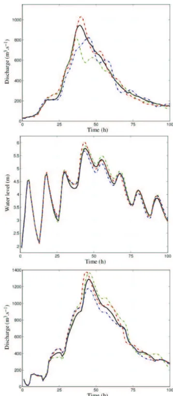
Alemohammad et al. (2015)proposed to reduce the input uncer-tain space with a singular vector decomposition applied to precip-itation fields to generate stochastic perturbation in position and magnitude.Li et al. (2016)used similar techniques (with empirical orthogonal functions) to reduce the size of the uncertain input space when quantifying uncertainties in initial and wind forcing uncertainties propagated by an ocean model. In the present study, upstream and downstream boundary conditions are perturbed using Gaussian processes, whose length scale is chosen in ade-quacy with the time scales of the hydraulic model. Downstream the hydraulic network, the water level is perturbed with a Gaus-sian noise characterized by a zero mean and a 6-h temporal corre-lation length scale that is coherent with the tidal cycle; the amplitude of the perturbation is set equal to the observation error at this observing station. At the upstream stations, the ensemble is generated by adding a Gaussian noise to the observed forcings. The observed upstream forcings are perturbed with a Gaussian noise characterized by a 4-h temporal auto-correlation length-scale, which was estimated with synthetic experiments. The amplitude of the perturbation is set equal to 15% of the discharge to account for the uncertainty in the rating curve that increases for high flow conditions.Fig. 4a illustrates the upstream forcing perturbation for three ensemble members at Escos during the 2011 flood event. The resulting perturbation of the water level and discharge at Peyreho-rade is displayed inFig. 4b and c, respectively.

3.3. EnKF implementation

The EnKF algorithm is implemented with OpenPALM3 (Buis et al., 2006; Piacentini et al., 2011). It is an open-source, flexible and powerful dynamic code coupler that has been jointly developed at CERFACS (Centre Européen de Recherche et Formation Avancée en Calcul Scientifique) and ONERA (Office National d’Etudes et de Recherches Aérospatiales) since 1996. OpenPALM provides a straightforward parallel environment based on high performance implementation of the Message Passing Interface standard (i.e.

MPICH, OpenMPI, LAM/MPI). This interface is able to perform both data parallelism (i.e. simultaneous execution on multiples cores of the same code component for a unique data set) and task parallelism (i.e. simultaneous execution on multiples cores of multiple tasks across the same or different data sets).

Task parallelism is particularly well adapted for the present

Fig. 4. (a) Time series of the upstream forcing on reach 6 during 2011 flood event: the black solid line corresponds to the observed ‘‘nominal” forcing; green, red and blue dashed lines correspond to perturbed forcings. The perturbation corresponds approximately to 15% of the nominal forcing. (b) Water levels and (c) discharges at Peyrehorade during 2011 flood event for the corresponding forcings.

Task parallelism is particularly well adapted for the present ensemble-based DA algorithm, where each MASCARET model

integration in the EnKF forecast step can be achieved indepen-dently of the others. The PalmParasol functionality in OpenPALM particularly addresses this need through the master/slaves princi-ple: the master processor spawns multiple copies of MASCARET (the slaves), each on one or several processors with a different set of input parameters (hydrological forcing in the present case). This allows for an efficient management of memory and processor allocation issues according to available resources.

3.4. Estimation of the observation error statistics

A method for the a posteriori estimation of the observation error is provided byLi et al. (2009)and is here applied to provide a more accurate description of the observation error variance than that prescribed to 10 cm inRicci et al. (2011). This estimation relies on the consistency criterion for R presented inDesroziers et al. (2005). Assuming that the matricesBandRare correct, the follow-ing relation holds:

hdo ad T o b i ¼ R; ð Þ4 where do b ¼ yo Hxb;1;. . .;yo Hxb N; e   and do a ¼ yo_{ Hx}a;1 ;. . .;yo_{ Hx}a N;e  

represent the forecast and analysis residuals with respect to the observation, respectively, and where h i: denotes the expectation operator.

In the present case, the observation error covariance matrixRis assumed to be diagonal with constant and uniform variance denoted by

r

2

o(since the measuring instruments are supposed to be independent and identical) with time invariant characteristics. Thus, Eq.(4)sums up to

hdo ad T o b i ¼

r

2

o: ð Þ5

When the size of the ensemble is limited, Eq.(5)cannot be used for a proper estimation of

r

_{o;Miyoshi (2005) and Li et al. (2009)}

proposed a method to accumulate information over successive assimilation cycles.

r

_{o obtained from Eq. (5)and the estimation}

r

b

oobtained from Eq.(6)over the previous assimilation cycle are combined using the following KF analysis equation, in which the control vector reduces to the scalar variable

r

_o:

r

a o¼ ð

m

o_Þ2

_r

b oþ ð

m

bÞ 2

_r

o ð

m

o_Þ2_{þ ð}

m

b_Þ2 ; ð Þ6 where

r

b

oand

r

aoare respectively the background and analyzed val-ues for

r

_oover the current assimilation cycle, and where

m

b_and

_m

o denote respectively the background and observation error STD for

r

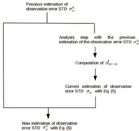
_{o. The flowchart of the}

r

_{o-estimation is given inFig. 5.}

The analyzed error STD for

r

_o is then given by the KF update equation in the scalar case:

ð

m

a Þ2¼ 1 ð

m

b_Þ2 ð

m

b_Þ2_{þ ð}

_m

o_Þ2 ! ð

m

b Þ2:

Regarding the KF forecast step, a persistence model is assumed for the dynamics of

r

oalong the assimilation cycles such that the background values for

r

oand its STD at time (i þ1) are obtained from the analysis time as follows:i

r

b o i;þ1¼

r

a o i;

m

b iþ1¼

j m

ai

A slow decrease of the error in

r

ois artificially prescribed with the parameter

j

_{¼ 1 03 as suggested in}: Li et al. (2009) Miyoshi.

(2005)showed that the final estimate of

r

_ois not sensitive to the values of

m

o _and

j

₍

j

_{> 1). Here}

m

b _{is initially set to 1 and}

m

o _is

This methodology is validated on a set of synthetic experiments in Section4.1.1. The observation error variance is estimated once and for all on real data in Section4.2.1.

3.5. Background error inflation

A common drawback of the EnKF is that when the size of the ensemble is limited, it tends to be under-dispersive and may diverge over time ignoring the observed information.Anderson and Anderson (1999)proposed to artificially increase the disper-sion within the ensemble by introducing a multiplicative inflation factor to the ensemble anomalies (the inflation factor increases the model state error variance at the observation point). Following this idea, we add inflation to the EnKF algorithm used for state estima-tion (IEnKF) in this study.

According to Anderson (2007), the difference between each member of the background ensemble xb _{and its mean can be} inflated using a time-varying inflation factork_>1, thus defining a new set of background states ~xb k; _{as well as a new set of} anoma-lies over which the background error covariance matrix can be computed:

~

xb k; _{ x}b_{¼ k x} b k; _{ x}b

: ð Þ7

The inflation factor is here derived from the consistency crite-k rion presented inDesroziers et al. (2005), based on the assumption that the errors in the background and observation error matrices are uncorrelated and properly described. In this context, the fol-lowing relation holds:

hdo bd T

o bi ¼ HBH

T_{þR: ð Þ8} In the literature,Li et al. (2009)proceeded to the simultaneous estimation of covariance inflation and observation errors. Here the observation error variance estimation described in Section3.4is achieved independently of the inflation coefficient computation.

Considering only one observation is assimilated, matrices in Eq.

(8)reduce to scalars: HBHT¼

r

2

b and R ¼

r

2o. If Eq.(8)does not hold and hdo bd

T o bi 

r

2o

 

>

r

2_{b, then the inflation factor is spec-}k ified as hdo bdTo bi ¼ k 2

_r

2 bþ

r

2 o; thus implying thatkverifies:

k2_¼hdo bd T o b i 

r

2 o

r

2 b ; ð Þ9

and the inflated background error variance at the observation point is increased to ~

r

_b2

¼ k2

r

2b. The inflation is then applied from the observation point to the entire computational domain (grid points are indexed with ) consistently with the shape of the correlationj functionCat the observation point using

~

xb k;_{ðjÞ  x}b_{ðjÞ ¼ 1 þ ðk  Þj ð Þjð 1 C j Þ x} b k;_{ðjÞ  x}b_{ð Þj}

 : ð10Þ

This formulation ensures that 1 þ ðk  Þj ð Þjð 1 C j Þ > 1, implying that the ensemble mean and the background error correlations over the computational domain are preserved and that the back-ground error covariances are locally increased in the vicinity of the observation point. The flowchart of the inflation procedure is given inFig. 6.

When No observations distributed over the hydraulic network are assimilated, the observation error matrix R is diagonal. The inflation equation now reads:

~ xb k;_{ðjÞ  x}b_{ðjÞ ¼ 1þ}XNo ðkn Þj1 Cnð Þjj ! xb k;_{ðjÞ  x}b_{ð Þj}  ; ð11Þ

values of

m

o _and

_j

₍

_j

_{> 1). Here}

_m

b _{is initially set to 1 and}

_m

o _is set to 0.85. X n¼1 !   where 1 þPNo

n¼1ðkn Þj1 Cnð Þjj is larger than 1 if kn> 1 for all obser-vation points (n ¼ ;1 . . .;No). If HBHT is not diagonal, a subset of observation points can be selected so that the matrix HBHTis diag-onal, thus reducing to the previous case. On the ‘‘Adour maritime” network, the model state error covariance functions have a large spatial extent so that the HBH T _{is never diagonal, that is why only}

3.6. Criteria for probabilistic forecast estimation

This section presents three criteria that are commonly used in meteorological applications to analyze probabilistic forecast per-formance (Talagrand et al., 1997). The consistency criterion charac-terizes the adequation between the distribution of the ensemble members and a set of observations through the use of the rank

his-Fig. 5. Flowchart of the sequential estimation of the observation error STD roover a given assimilation cycle.

spatial extent so that the HBH is never diagonal, that is why only

one observing point is used to compute the inflation factor k. memberstogram for a given forecast lead time. Over a flood event for which and a set of observations through the use of the rank

his-the DA algorithm is sequentially applied, his-the forecast values are ranked in increasing order defining ðNeþ Þ1 classes. Then the occurrence of the observed values within these classes is repre-sented as a histogram. A flat histogram is satisfactory and means that the ensemble members and the observations follow similar distributions. In contrast, a U-shape histogram means that the ensemble is under-dispersive.

The reliability criterion evaluates the coherence between the forecasted and observed probabilities of an event. An event is defined as Z_f PZ_{Tg, where}Zis the random variable forecast value and ZTis a threshold value. The reliability plot represents the pos-terior observation frequency with respect to the prior forecast probability for a given forecast lead time. The ensemble is reliable if this relation follows the first bisector; it is under- or over-predictive otherwise.

The accuracy criterion characterizes the ability of the forecast to describe the reality through the well-known Brier score (Brier, 1950). Nonetheless, for the Brier score the set of possible outcomes is binary, for example: was the forecast water level higher than a given threshold? In this study, as the observations spread covers a wide range of values, the CRPS (Continuous Rank Probability Score) is used; its expression is given by

CRPS ¼1 T X T t¼1 Z R FpðxÞ  Foð Þx  2 dx;

with Fpthe ensemble cumulative distribution function (CDF) and FoðxÞ ¼ 1½y;þ1½ð Þx the observation CDF. The CRPS is computed for dif-ferent lead times and is expected to increase with the forecast lead time.

Examples of consistency rank histogram, reliability plot and accuracy plot are provided inFigs. 7 and 8at Peyrehorade. 3.7. Data assimilation experiments

For verification purposes, experiments representative of the ‘‘Adour Maritime” conditions are first carried out in the framework of OSSE and are referred to as DA-OSSE; experiments assimilating real water level measurements along the river network are referred to as DA-REAL.

3.7.1. Description of DA-OSSE

DA-OSSE1 experiments (Section 4.1.1) show how to properly estimate observation error statistics following the methodology presented in Section3.4. Synthetic upstream forcings that are rep-resentative of the ‘‘Adour Maritime” non-flooding conditions are used: 50 m3s1 _{at Dax and Escos, 70 m}3

s1 _{at Orthez and} 20 m3_s1_{at Cambo. MASCARET is integrated for these reference} forcings and a Gaussian noise is added to the water level simula-tions at the observing stasimula-tions to generate synthetic observasimula-tions. Perturbations are introduced to these reference forcings to gener-ate an ensemble of wgener-ater level simulations.

DA-OSSE2 experiments (Section4.1.2) test in forecast mode, the consistency, reliability and accuracy properties of the ensemble presented in Section 3.6on the eight flood events available on the ‘‘Adour Maritime” network. For each event, upstream per-turbed forcings are set up using time series observed during the flood events. MASCARET is integrated for these observed forcings and a Gaussian noise (with observation error STD computed in Sec-tion4.2.1) is added to the simulated water level at the observing stations to generate synthetic observations.

DA-OSSE3 (Section 4.1.3) mimics real conditions on the ‘‘Adour Maritime” river network, where uncertainties on lateral inflows are important during flood events such as 2011 flood event. The refer-ence upstream forcings are set up using the observed forcings and

maximum discharge of 575 m3_s1_{. A Gaussian noise is added to} the MASCARET simulation outputs at the observing stations. Each background member results from the integration of each upstream and the lateral inflow is removed.

3.7.2. Description of DA-REAL

In DA-REAL1 (Section4.2.1), realistic observation error statistics are derived from a case in which upstream forcings provided by observations are almost constant (50 m3s1 _{at Dax and Escos,} 70 m3_s1 _{at Orthez and 20 m}3_s1 _{at Cambo). The ensemble is} based on perturbed upstream forcings; the IEnKF assimilates water level observations at the observing stations of Peyrehorade and Pont-Blanc with a maximum lead time of 12 h that correspond to the maximum transfer time of the network.

In DA-REAL2 (Section4.2.2), the performance of the IEnKF algo-rithm is evaluated against the eight flood events in terms of RMSE time series and illustrated on the 2014 flood event.

For DA-OSSE1, DA-OSSE3 and DA-REAL, 40 members are gener-ated (numerical experiments not reported here show that 40 mem-bers are sufficient to properly estimate covariance functions). For DA-OSSE2, only 16 members were used to circumvent the lack of available data and provide a correct estimation.

4. Results

4.1. Synthetic experiment results (DA-OSSE) 4.1.1. Estimation of observation error STD

The observation error STD

r

_ois estimated by applying the crite-ria presented in Section3.4to DA-OSSE1 (the same approach is applied to DA-REAL in Section4.2.1). We consider three different values for

r

_o: 0.025, 0.075 and 0.125 m. The methodology is applied sequentially over 150 assimilation cycles (this corresponds approximately to 6 days for a 1-h DA frequency). The estimated value of

r

oreported inTable 1is computed as the mean value com-puted for

r

_{obetween cycles 50 and 150, a time period over which}

the estimation of

r

_oconverges.Table 1shows that the observation error STD

r

_{ocan be accurately retrieved with a relative error of less}

than 5 2 .: %

4.1.2. Estimation of ensemble forecast properties

The quality of ensemble forecasts is estimated by applying the methodology presented in Section3.6to DA-OSSE2.

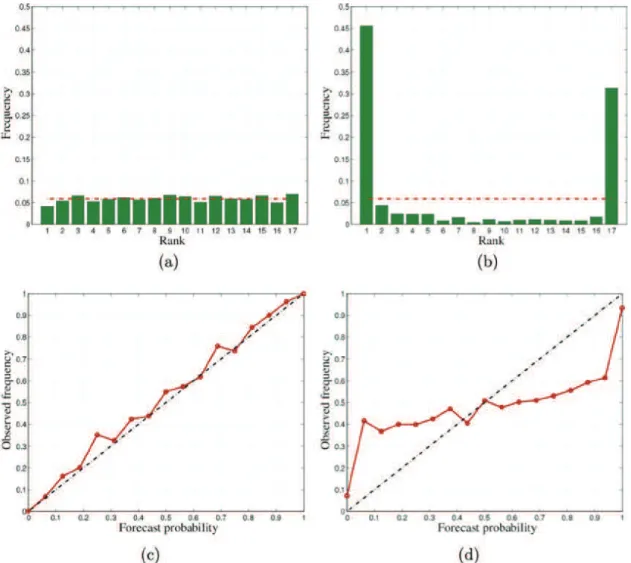
The rank histogram displayed inFig. 7a for a 5-h forecast lead time that is shorter than the transfer time at Peyrehorade (6 h) is nearly flat. This implies that the ensemble and the observations follow the same random variable for this lead time; water level forecast can be therefore provided with uncertainty range (for example, with STD or with box plots).

Even though several synthetic flood events are used in DA-OSSE2, because of the lack of data for flood peaks, it is not possible to evaluate the reliability property for a single probabilistic event of the type Zf PZTg. Nonetheless, since there is no model error and no bias on the forcings in DA-OSSE2, since error observations are homogeneous, reliability is evaluated on a set of events

ZPZk_T n o

, where ZkT covers different threshold values ZT. The reli-ability line in Fig. 7c is close to the identity line, meaning that fore-cast probabilities are in agreement with observed frequencies for this lead time. When the forecast lead time (here 12 h) is longer than the transfer time, the ensemble is not consistent with the observations, nor reliable as shown in Fig. 7b-d. This is due to the unrealistic description of the inflow as the upstream forcings are set constant beyond the last observed time. The ensemble is

ence upstream forcings are set up using the observed forcings and a synthetic lateral inflow on reach 6.This lateral inflow reaches a

are set constant beyond the last observed time. The ensemble is deemed under-dispersive, under-predictive for forecast

probabili-ties lower than 0.5 and over-predictive for forecast probabilities

Fig. 8shows that the forecast accuracy rapidly decreases when the forecast lead time exceeds the transfer time (for example 5 h at Peyrehorade). This is particularly true where the sensitivity to the upstream forcings is large. In the present case, since the water level at Lesseps is more sensitive to the downstream boundary condition than to the upstream one, the forecast accuracy remains satisfying, even when upstream forcings are unrealistic (beyond 12 h).

4.1.3. Hydraulic state estimation

4.1.3.1. Comparison of EnKF and IEnKF. The capability of the IEnKF to compute accurate water level and discharge is assessed in DA-OSSE3. This setting is closer to operational conditions where there are various sources of uncertainty such as those related to lateral inflows. The objective is to show the merits of inflation to compute correct water level and discharge, even with important error on lateral inflows, through a comparison between IEnKF and EnKF

Fig. 7. DA-OSSE2 experiment – Ensemble forecast properties at the Peyrehorade station at 5-h (left panels) and 12-h (right panels) forecast lead times. (a)-(b) Rank diagram. (c)-(d) Reliability diagram.

Fig. 8. DA-OSSE2 experiment – CRPS for lead times from 1 to 12 h at Peyrehorade (red line) and Lesseps (green line) stations.

Table 1

Prescribed and estimated observation error STDrofollowing methodology presented

in Section3.4 , i.e. with the following parametersj¼ 1 03: ;mb_{¼ 1 andm}o_{¼ 0 85 – DA-:}

OSSE1 experiment.

Prescribedr_o(m) 0.025 0.075 0.125 Estimatedr_o(m) 0.0263 0.0748 0.13125

ties lower than 0.5 and over-predictive for forecast probabilities larger than 0.5.

lateral inflows, through a comparison between IEnKF and EnKF results in Fig. 9.

In the EnKF (green curve), as the size of the sample is limited, the uncertainty description is only partial and the ensemble tends to collapse as observations are assimilated. As a consequence, the variance of the model ensemble decreases along DA cycles in

Fig. 9and the observations have a smaller impact on the analysis. This is a common drawback of the EnKF (in the extreme case obser-vations are ignored by the DA analysis).

The inflation approach (red curve) is an artificial way to over-come this limitation adding some dispersion within the ensemble members. The ensemble variance is reduced as observations are assimilated as expected with DA; still, the IEnKF forecast step is able to input enough dispersion with in the ensemble so that the variance of the ensemble remains large enough for observations to have an impact on the following DA analysis cycle.

Fig. 9 illustrates that the difference between analyzed water level and water level observations is more efficiently reduced by IEnKF (red curve) than by EnKF (green curve), especially when the discrepancy between the model free run (black curve) and the observations (blue curve) is large. This justifies the use of IEnKF rather than EnKF. In the following, the shape, the temporal and spatial variability of the covariance functions for IEnKF is studied here and compared to that of deterministic IKF algorithm (Ricci et al., 2011).

4.1.3.2. Covariance functions. The 2011 flood event lasted more than 6 days (about 150 h) and decomposes in two flood peaks. The covariance functions are analyzed for two different times, before the first flood peak at 25 h and during the second flood peak at 100 h. Note that the time is given with respect to the flood start.

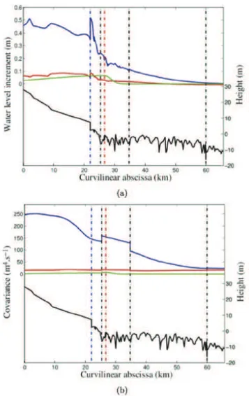
Fig. 10a displays the background error univariate covariance func-tion related to water level (term BZZ, Section3.1) andFig. 10b dis-plays the background error multivariate covariance function related to water-level/discharge variables (term BQZ, Section3.1) associated with the observing station at Peyrehorade. These func-tions are presented along reaches 6–5-2–1 for the IKF (green lines) and for the IEnKF at times 25 h (red line) and 100 h (blue line).

The IEnKF water level univariate covariance function shows important discontinuity where the river geometry features abrupt and frequent changes, for instance at the dam location on reach 6 (vertical blue dashed line) as well as at the river network upstream where the bathymetry profile is smoother with a large, relatively

tidal influence, the covariance function is smooth and decreases. The IKF covariance function presents significantly shorter correla-tion length scales than that of the IEnKF, especially downstream of the observation point, and has no coherence with the river geometry by construction.

The IEnKF water level/discharge multivariate covariance func-tion presents a discontinuity at each confluence between reaches (vertical black dashed line) since discharge is an additive variable. It also features larger spatial extent than that of the IKF function. It is worth mentioning that in the IKF, the water level/discharge mul-tivariate relation is prescribed with a proportionality coefficient between the ratio of the water level and discharge increments and the ratio of the background water level and discharge values at the observing station; discharge conservation is thus explicitly preserved at confluences.

4.1.3.3. Water level and discharge analysis increments. The mean (ensemble-averaged) water level and discharge increments obtained through the IEnKF and IKF analysis steps at time 25 h (red lines) and time 100 h (blue lines) are shown in Fig. 11. The

0 0.1 0.2 0.3 0.4 Time (h)

Mean AMO (m) Water level (m)

0 20 40 60 80 100 120 140 160 180 3 4 5 6 7

Fig. 9. DA-OSSE3 experiment – Difference between analyzed and observed water levels at Peyrehorade for 2011 event for EnKF (green curve) and IEnKF (red curve). The model free run (black curve) and observations (blue curve) are plotted in the right y-axis.

Fig. 10. DA-OSSE3 experiment – (a) Water level covariance function associated with analysis at Peyrehorade at time 25 h (solid red line) and at time 100 h (blue solid line) with the IEnKF. The time-invariant counterpart for the IKF is given in green solid line. (b) Same caption as (a) for water-level/discharge covariance function. Vertical red dashed lines represent the Peyrehorade observing station. Vertical black dashed lines represent the separation between two reaches corre-sponding to confluences. Vertical blue dashed lines represent the dam position on reach 6. Black solid lines correspond to bathymetry (right y-axis).

where the bathymetry profile is smoother with a large, relatively

uniform slope. Downstream of the dam, the Adour river is under (redIEnKF lines) and time 100 h (blue lines) are shown in corrections are consistent with the previously-describedFig. 11. The

covariance functions and thereby with the network geometric properties (see the bathymetry profile in continuous black line in

Fig. 10a-b, right -axis). They provide an optimal and spatially-y distributed correction in water level and discharge. As the error correlation length scales are large, the impact of a local observation is spread onto the entire hydraulic network, both for water level and discharge. The corrected hydraulic state is thus used as initial condition for further forecast and in particular for the next assim-ilation cycle.

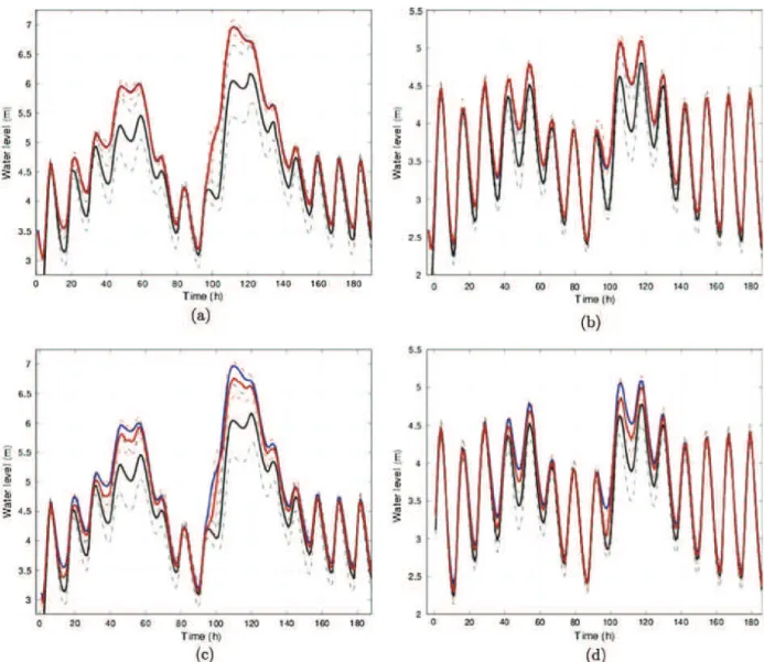
4.1.3.4. Water level and discharge analysis. In the following, results are presented in terms of the time-evolving mean water level/dis-charge computed over the ensemble, which results from the IEnKF sequential application in the context of DA-OSSE3 experiment. Fig. 12a-b show the water level temporal evolution at Peyrehorade and Urt during the whole 2011 flood event in terms of ensemble means (red solid lines) and STD (red dotted thin lines). In the pre-sent case, only observations at Peyrehorade are assimilated in order to highlight the impact of the spatial correction due to the

assimilated). IEnKF results at the analysis time are compared to the MASCARET standalone simulation (black line – referred to as free run and corresponding to a case without DA) and to the avail-able observations (blue line) over the 6 days.Fig. 13a-b present the counterpart ofFig. 12a-b for the river discharge. At the analysis time, the water level at Peyrehorade and Urt is brought closer to the observations than the free run. The discharge is also signifi-cantly improved at both observing stations. The spread of the water level and discharge ensemble is significantly reduced with DA, showing that DA reduced uncertainty at the analysis time.

Fig. 12c presents the counterpart ofFig. 12a for the 2-h forecast water level (at Peyrehorade). In addition, Fig. 12d presents the counterpart of Fig. 12b for the 4-h forecast water level (at Urt). The objective is to analyze how the IEnKF performance varies with respect to the forecast lead time. While a significant improvement is obtained for short-range forecast (1 to 3-h forecast) on the water level ensemble mean, the improvement resulting from the IEnKF decreases as the forecast lead time increases since the persistence of the hydraulic state correction is limited in time. For increasing lead time, the analyzed water level thus drifts back towards the free run because of model uncertainties (forcing, geometry, fric-tion); the assimilation is less efficient in reducing uncertainty and thus the ensemble spread. This highlights the need to extend the control vector to model parameters and hydrological forcing to improve medium- to long-range forecasts (3 to 6-h forecast and 6 to 24-h forecast, respectively). Beyond the transfer time of the upstream forcing, the error in the forecast water level signifi-cantly increases as unrealistic forcings are input to the system.

4.1.3.5. Intermediate conclusions and discussion. The DA-OSSE3 results on the 2011 flood event show that (1) a water level obser-vation (here at Peyrehorade) is translated into a spatial correction in water level and discharge; (2) the analysis is coherent with the reference state; and (3) it is better than the free run, even where no observations are available (here at Urt) and for variables that are not assimilated (i.e. river discharge). While this provides a proper validation of the IEnKF algorithm, it should be noted that in the framework of real DA, the ensemble-based estimation of the uni-variate and multiuni-variate covariance functions may lead to a smaller improvement. Indeed, the estimation of these functions relies on the quality of the model. For instance, if the description of the bathymetry or the friction coefficient is erroneous, the water level/discharge relation in the model may be inconsistent with that of the reality and the DA algorithm may fail to derive a satisfactory increment over the entire network for both variables from a lim-ited number of assimilated observations. This is the advantage of the OSSE framework; the water level/discharge relation within the model is similar to that of the observations. This will be further discussed in Section4.2.

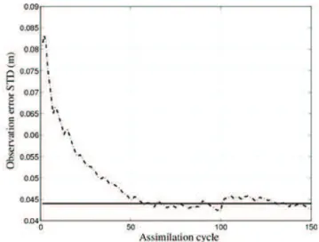
4.2. Real data experiment results (DA-REAL) 4.2.1. Estimation of observation error STD

To estimate the observation error STD

r

_o with real data (DA-REAL1), we selected data with small error in the hydrological forc-ings so that the model error at the observing stations is small.

r

_o is estimated through successive DA cycles with the same method as presented in Section 4.1.1for DA-OSSE1 experiments. It is found that the estimated

r

_o (black dashed line in Fig. 14) converged to 0.044 m (continuous black line in Fig. 14); this value is obtained as the average value between assimilation cycles 60 to 150. Thus, in the following DA-REAL experiments, the observation error STD

Fig. 11. DA-OSSE3 experiment – (a) Analyzed water level increment associated with analysis at Peyrehorade at time 25 h (solid red line) and at time 100 h (blue solid line) with the IEnKF. The time-invariant counterpart for the IKF is given in green solid line. (b) Same caption as (a) for discharge increment. Vertical red dashed lines represent the location of Peyrehorade station. Vertical black dashed lines represent the separation between two reaches corresponding to confluences. Vertical blue dashed lines represent the dam position on reach 6. Black solid lines correspond to bathymetry (right y-axis).

order to highlight the impact of the spatial correction due to the

covariance functions (in real cases all available observations are in

r

o is the following DA-REAL experiments, the observation error STD fixed constant and equal to 0.044 m.

Fig. 12. DA-OSSE3 experiment – Ensemble water level at (a)-(c) Peyrehorade and (b)-(d) Urt. (a)-(b) correspond to the analysis time (+0-h forecast lead time). (c) corresponds to the 2-h forecast lead time. (d) corresponds to the 4-h forecast lead time. Solid red lines represent the mean IEnKF estimate; red dotted lines represent the ensemble STD; blue lines represent observations; black lines represent the free run mean; and black dotted lines represent the STD of the ensemble free run. (For interpretation of the references to colour in this figure legend, the reader is referred to the web version of this article.)

4.2.2. Hydraulic state estimation

In the context of DA-REAL2, the IEnKF is evaluated against a set of eight flood events on the Adour catchment from 2009 to 2014. Hourly water level observations were assimilated at Peyrehorade and Pont-Blanc. In the following, results are presented for the 2014 event that is characterized by a simultaneous flood peak on reaches 3–6-7 (Cambo, Escos, Orthez, respectively) followed by a flood peak on reach 4 (Dax).Fig. 15a-b present the time-evolving observed river discharge at upstream stations and the time-evolving water level at the downstream stations.

Water level results of the sequential application of the IEnKF for the 2014 flood event are displayed inFig. 16a-b at Peyrehorade and Urt, respectively. At the analysis time (+0-h forecast lead time), the assimilation leads to excellent results and the water level at Peyre-horade is as satisfying as in DA-OSSE3 experiment. The improve-ment at Urt is less obvious: the water level is improved, except close to the flood peak that remains overestimated. At the begin-ning of the flood event, the lack of flood plain modeling near Urt is penalizing and the infinite banks assumption in the 1D model results in an erroneous water line dynamic that causes errors in

Fig. 14. DA-REAL1experiment – Iterative estimation of the observation error STD

r_{oalong assimilation cycles (dashed line) and the resulting reference value 0.044 m}

(solid line).

Fig. 15. DA-REAL2 experiment – (a) Discharge time series at upstream stations and

Fig. 16. DA-REAL2 experiment – Ensemble water level comparison at (a) Peyreho-rade and (b) Urt for the 2014 flood event. The mean analysis is represented in red

(b) water level time series at the downstream station over the 2014 flood event. See

Fig. 1for a scheme of the ‘‘Adour Maritime” network.

line; the observations are represented in blue; and the mean free run is represented in black.

the water level covariance functions. Thus, in spite of the assimila-tion of observed water level at Peyrehorade, the simulated water level at Urt remains overestimated for high flow on reaches 6 and 7. After the flood peak, for medium flow, MASCARET predic-tions are realistic and the simulated water level is improved at Urt.

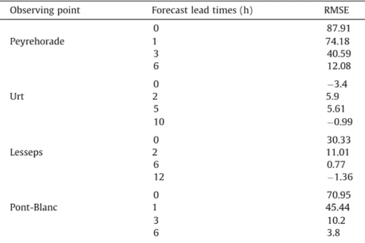
Table 2 summarizes the improvement in the mean RMSE obtained thanks to the IEnKF for the eight flood events, for forecast lead times ranging from 0 to 12 h depending on the observing sta-tion on the hydraulic network. Assimilating observasta-tions at Peyre-horade and Pont-Blanc significantly improves the water level RMSE for short- to medium-range lead time at these locations. The water level is also improved at Lesseps, where no observation is assimi-lated. However, the impact at Urt is not significant on average due to model errors in this area.

5. Conclusion and discussion

This study describes the application of the EnKF algorithm on the ‘‘Adour Maritime” hydraulic network (South West France) using the 1D hydrodynamic code MASCARET.

Results show that flow dependent error covariance statistics are accurately estimated using only 40 ensemble members. The model state functions are found to be closely related to the network geometry as well as the hydrological forcing; one interesting prop-erty is that they are characterized by an important spatial extent. To increase EnKF performance, two additional algorithms esti-mating observation and background error covariances at the observing stations were implemented. The resulting algorithm is referred to as the IEnKF. It is shown on a set of synthetic experi-ments that, under the assumption that the observation error is constant, the observation error STD can be accurately estimated. Using real data, a realistic observation error STD was estimated at 4.4 cm on the ‘‘Adour Maritime” network. Additionally, back-ground error inflation was found efficient to properly represent the error variability in the hydraulic state and to avoid EnKF col-lapse and divergence from the observations.

Results showed on a synthetic experiment with ungauged lat-eral inflow that the IEnKF data-driven model provided better results, in terms of analyzed and forecast water level and discharge for short forecast lead times (1 to 3 h), compared to the free run. Experiments with a set of eight recent flood events (2009–2014) provided good results at the stations where the assimilation is

per-overestimated because of the lack of flood plain in the ‘‘Adour Mar-itime” hydraulic model.

Properties of probabilistic forecast with IEnKF on the ‘‘Adour Maritime” network were then examined on several synthetic flood events through three criteria: consistency, reliability and accuracy. Under the assumption that the only source of uncertainty lies in observation error, probabilistic forecasts were correctly estimated according to these criteria for forecast lead times shorter than the transfer time of upstream forcings along the network.

Nonetheless, this study features several limitations. First, the lack of flood plain in the ‘‘Adour Maritime” hydraulic model results in a mis-estimation of the model state covariance functions and can lead to the result degradation in the correlation area of the sta-tion where observasta-tions are assimilated. Efforts are ongoing at SPG GAD to overcome this modeling limitation. Another limitation on the ‘‘Adour Maritime” network lies in the uncertainties in the forc-ings. On the one hand, there are ungauged lateral inflows (such as Bidouze or Luy rivers) whose contributions can be very important during flood events and which are not accounted for in the present hydraulic network. On the other hand, correcting errors in the forc-ings has a limited impact in forecast mode as the correction is propagated downstream and finally exits the network.

Despite those limitations, this study presents several perspec-tives. The IEnKF strategy presented here could be applied to 2D hydraulic modeling that also suffers from uncertain hydrological forcings; for instance, the correction could be extended to pressure and wind surface forcings. In this context, the need to reduce the uncertain input space dimension would be even more crucial for generating coherent ensemble and representative flow dependent background error covariance functions (the flow may move from the river bed to the flood plains). Another direct application is to supply corrected boundary conditions for 2D hydraulic models in the context of multi-dimensional (1D-2D) hydrodynamic model combined with DA on the 1D model. Multi-dimensional coupling with IEnKF on the 1D model is a promising approach to improve short-term (1–3 h) forecast performance as highlighted by ongoing studies on the ‘‘Adour Maritime” network.

Acknowledgments

The financial support provided by SCHAPI and ‘‘Région Midi-P yrénées” was greatly appreciated. The authors also gratefully acknowledge Thierry Morel and Florent Duchaine (CERFACS) for their support on OpenPALM and on the PalmParasol functionality.

References

Alemohammad, S., McLaughlin, D., Entekhabi, D., 2015. Quantifying precipitation uncertainty for land data assimilation applications. Mon. Weather Rev. 143, 3276–3299.http://dx.doi.org/10.1175/MWR-D-14-00337.1.

Anderson, J.L., 2007. An adaptive covariance inflation error correction algorithm for ensemble filters. Tellus, Series A: Dyn. Meteorol. Oceanogr. 59, 210–224.http:// dx.doi.org/10.1111/j.1600-0870.2006.00216.x. ISSN 02806495.

Anderson, J.L., Anderson, S.L., 1999. A Monte Carlo implementation of the nonlinear filtering problem to produce ensemble assimilations and forecasts. Mon. Weather Rev. 127, 2741–2758. http://dx.doi.org/10.1175/1520-0493(1999) 127<2741:AMCIOT>2.0.CO;2. ISSN 0027-0644.

Andreadis, K.M., Clark, E.A., Lettenmaier, D.P., Alsdorf, D.E., 2007. Prospects for river discharge and depth estimation through assimilation of swath-altimetry into a raster-based hydrodynamics model. Geophys. Res. Lett. 34, 1–5.http://dx.doi. org/10.1029/2007GL029721. ISSN 00948276..

M. Audinet, H. André, 1995. Hydrométrie appliquée aux cours d’eau, Collection EDF-DER no. 91.

Biancamaria, S., Durand, M., Andreadis, K.M., Bates, P.D., Boone, A., Mognard, N.M., Rodr´guez, E., Alsdorf, D.E., Lettenmaier, D.P., Clark, E.A., 2011. Assimilation of virtual wide swath altimetry to improve Arctic river modeling. Remote Sensing Environ. 115 (2), 373–381. http://dx.doi.org/10.1016/j.rse.2010.09.008. ISSN 00344257.

Table 2

Percentage mean improvement of the water level RMSE at the stations of Peyreho-rade, Urt, Lesseps and Pont-Blanc for increasing forecast lead times from 0-h to 12-h.

Observing point Forecast lead times (h) RMSE

0 87.91 Peyrehorade 1 74.18 3 40.59 6 12.08 0 3.4 Urt 2 5.9 5 5.61 10 0.99 0 30.33 Lesseps 2 11.01 6 0.77 12 1.36 0 70.95 Pont-Blanc 1 45.44 3 10.2 6 3.8

provided good results at the stations where the assimilation is per-formed, but the water level computed at other stations may be

00344257.

Bozzi, S., Passoni, G., Bernardara, P., Goutal, N., Arnaud, A., 2014. Roughness and discharge uncertainty in 1D water level calculations. Environ. Modeling Assess.

4.http://dx.doi.org/10.1007/s10666-014-9430-6. ISSN 1420–2026, URLhttp:// link.springer.com/10.1007/s10666-014-9430-6.

Brier, G.W., 1950. Cerification of forecasts expressed in terms of probaility. Mon. Weather Rev. 78 (1), 1–3.http://dx.doi.org/10.1126/science.27.693.594. ISSN 0036–8075.

Buis, S., Piacentini, A., Déclat, D., 2006. PALM: a computational framework for assembling high-performance computing applications. Concurrency Comput.: Pract. Exp. 18 (2), 231–245.

Burgers, G., Jan van Leeuwen, P., Evensen, G., 1998. Analysis scheme in the ensemble Kalman filter. Mon. Weather Rev. 126 (6), 1719–1724. ISSN 0027–0644. Desroziers, G., Berre, L., Chapnik, B., Poli, P., 2005. Diagnosis of observation,

background and analysis-error statistics in observation space. Q. J. R. Meteorol. Soc. 131 (2005), 3385–3396. http://dx.doi.org/10.1256/qj.05.108. ISSN 00359009, URLhttp://doi.wiley.com/10.1256/qj.05.108.

Dumedah, G., Walker, J., 2017. Assessment of model behavior and acceptable forcing data uncertainty in the context of land surface soil moisture estimation. Adv. Water Resour. 101, 23–36. http://dx.doi.org/10.1016/j. advwatres.2017.01.001.

Durand, M., Andreadis, K.M., Alsdorf, D.E., Lettenmaier, D.P., Moller, D., Wilson, M., 2008. Estimation of bathymetric depth and slope from data assimilation of swath altimetry into a hydrodynamic model. Geophys. Res. Lett. 35, 1–5.http:// dx.doi.org/10.1029/2008GL034150. ISSN 00948276.

Evensen, G., 1994. Sequential data assimilation with a nonlinear quasi-geostrophic model using Monte Carlo methods to forecast error statistics. J. Geophys. Res. 99 (C5), 10143–10162.http://dx.doi.org/10.1029/94JC00572. ISSN 0148– 0227.

Giustarini, L., Matgen, P., Hostache, R., Montanari, M., Plaza, D., Pauwels, V.R.N., De Lannoy, G.J.M., De Keyser, R., Pfister, L., Hoffmann, L., Savenije, H.H.G., 2011. Assimilating SAR-derived water level data into a hydraulic model: a case study. Hydrol. Earth Syst. Sci. 15, 2349–2365. http://dx.doi.org/10.5194/hess-15-2349-2011. ISSN 10275606.

Goutal, N., Maurel, F., 2002. A finite volume solver for 1D shallow-water equations applied to an actual river. Int. J. Numer. Methods Fluids 38 (1), 1–19. Guha-Sapir, D., Vos, F., Below, R., Penserre, S., 2012. Annual disaster statistical

review 2011: the numbers and trends. Cred 2010 (384). URLhttp://www.cred. be/sites/default/files/ADSR2011.pdf.

Habert, J., Ricci, S., Le Pape, E., Thual, O., Piacentini, A., Goutal, N., Rochoux, M., 2016. Reduction of the uncertainties in the water level-discharge relation of a 1D hydraulic model in the context of operational flood forecasting. J. Hydrol.

J. Hartnack, H. Madsen, J. Tornfeldt Sorensen, 2005. DATA ASSIMILATION IN A COMBINED 1D–2D FLOOD MODEL, Tech. Rep.

Jean-Baptiste, N., Malaterre, P.O., Dorée, C., Sau, J., 2011. Data assimilation for real-time estimation of hydraulic states and unmeasured perturbations in a 1D hydrodynamic model. Math. Comput. Simul. 81 (10), 2201–2214.http://dx.doi. org/10.1016/j.matcom.2010.12.021. ISSN 03784754.

Li, G., Iskandarani, M., Le Henaff, M., Winokur, J., Le Maıtre, O., Knio, O., 2016. Quantifying initial and wind forcing uncertainties in the Gulf of Mexico. Comput. Geosci. 20 (5), 1133–1153. http://dx.doi.org/10.1007/s10596-016-9581-4.

Li, H., Kalnay, E., Miyoshi, T., 2009. Simultaneous estimation of covariance inflation and observation errors within an ensemble Kalman filter. Q. J. Royal 135 (February), 523–533.http://dx.doi.org/10.1002/qj.371.

Madsen, H., Skotner, C., 2005. Adaptive state updating in real-time river flow forecasting – A combined filtering and error forecasting procedure. J. Hydrol. 308, 302–312.http://dx.doi.org/10.1016/j.jhydrol.2004.10.030. ISSN 00221694. Maggioni, V., Anagnostou, E., Reichle, R., 2012. The impact of model and rainfall forcing errors on characterizing soil moisture uncertainty in land surface

modeling. Hydrol. Earth Syst. Sci. 16, 3499–3515.http://dx.doi.org/10.5194/ hess-16-3499-2012.

Matgen, P., Montanari, M., Hostache, R., Pfister, L., Hoffmann, L., Plaza, D., Pauwels, V.R.N., De Lannoy, G.J.M., De Keyser, R., Savenije, H.H.G., 2010. Towards the sequential assimilation of SAR-derived water stages into hydraulic models using the Particle Filter: Proof of concept. Hydrol. Earth Syst. Sci. 14, 1773– 1785.http://dx.doi.org/10.5194/hess-14-1773-2010. ISSN 10275606. Miyoshi T., 2005. Ensemble Kalman Filter Experiments With a Primitive-Equation

Global Model, Doctor

Neal, J.C., Schumann, G., Bates, P.D., Buytaert, W., Matgen, P., Pappenberger, F., 2009. A data assimilation approach to discharge estimation from space. Hydrol. Process. 23, 3641–3649.http://dx.doi.org/10.1002/hyp.7518. URLhttp://jamsb. austms.org.au/courses/CSC2408/semester3/resources/ldp/abs-guide.pdf. Piacentini, A., Morel, T., Thévenin, A., Duchaine, F., 2011. O-Palm: An open source

dynamic parallel coupler. In: Proceedings of the 4th International Conference on Computational Methods for Coupled Problems in Science and Engineering, COUPLED ProblemS 2011 URLhttp://www.scopus.com/inward/record.url?eid= 2-s2.0-84857394958&partnerID=40&md5=

68a5bee3be07572776ea8cd9dd6240a3.

Ricci, S., Piacentini, A., Thual, O., Le Pape, E., Jonville, G., 2011. Correction of upstream flow and hydraulic state with data assimilation in the context of flood forecasting. Hydrol. Earth Syst. Sci. 15, 3555–3575.http://dx.doi.org/10.5194/ hess-15-3555-2011. ISSN 10275606.

Roe, P., 1981. Approximate Riemann solvers, parameter vectors, and difference schemes. J. Comput. Phys. 43, 357–372.http://dx.doi.org/10.1016/0021-9991 (81)90128-5. ISSN 00219991, URL http://www.sciencedirect.com/science/ article/pii/0021999181901285.

Shiiba, M., Laurenson, X., Tachikawa, Y., 2000. Real-time stage and discharge estimation by a stochastic-dynamic flood routing model, Hydrological Processes 14 (February 1999) (2000) 481–495, ISSN 08856087, doi: 10.1002/(SICI)1099-1085(20000228)14:3481::AID-HYP9503.0.CO;2-F.

Stocker, T., Qin, D., Plattner, G., Tignor, M., Allen, S., Boschung, J., Nauels, A., Xia, Y., Bex, B., Midgley, B., 2013. IPCC, 2013: climate change 2013: the physical science basis. Contribution of working group I to the fifth assessment report of the intergovernmental panel on climate change.

Talagrand, O., Vautard, R., Strauss, B., 1997. Evaluation of probabilistic prediction systems, in: Proc. ECMWF Workshop on Predictability, 1–25.

Vrugt, J.A., ter Braak, C.J.F., Clark, M.P., Hyman, J.M., Robinson, B.A., 2008. Treatment of input uncertainty in hydrologic modeling: Doing hydrology backward with Markov chain Monte Carlo simulation. Water Resources Research 44 (W00B09).

http://dx.doi.org/10.1029/2007WR006720. ISSN 00431397, URL http://doi. wiley.com/10.1029/2007WR006720.

Weerts, A.H., Winsemius, H.C., Verkade, J.S., 2011. Estimation of predictive hydrological uncertainty using quantile regression: examples from the National Flood Forecasting System (England and Wales). Hydrol. Earth System Sci. 15, 255–265. http://dx.doi.org/10.5194/hess-15-255-2011. ISSN 1607-7938, URLhttp://www.hydrol-earth-syst-sci.net/15/255/2011/.

Werner, M., Cranston, M., Harrison, T., Whitfield, D., Schellekens, J., 2009. Recent developments in operational flood forecasting in England, Wales and Scotland. Meteorol. Appl. 16 (February), 13–22.http://dx.doi.org/10.1002/met.124. World Meteorological Organization, Manual on flood forecasting and warning,

1072, ISBN 9789263110725, 2011.

Yoon, Y., Durand, M., Merry, C.J., Clark, E.A., Andreadis, K.M., Alsdorf, D.E., 2012. Estimating river bathymetry from data assimilation of synthetic SWOT measurements. J. Hydrol. 464-465, 363–375. http://dx.doi.org/10.1016/j. jhydrol.2012.07.02. ISSN 00221694, URL http://dx.doi.org/10.1016/j.jhydrol. 2012.07.028.