To link to this article:
DOI:10.1080/00207543.2017.1308575
URL:
https://doi.org/10.1080/00207543.2017.1308575
This is an author-deposited version published in:
http://oatao.univ-toulouse.fr/
Eprints ID:
19719
To cite this version:
Khemiri, Rihab and Elbedoui-Maktouf, Khaoula and Grabot, Bernard and
Zouari, Belhassen A fuzzy multi-criteria decision making approach for
managing performance and risk in integrated procurement-production
planning. (2017) International Journal of Production Research, vol. 55
(n°18). pp. 5305-5329. ISSN 0020-7543
O
pen
A
rchive
T
oulouse
A
rchive
O
uverte (
OATAO
)
OATAO is an open access repository that collects the work of Toulouse researchers and
makes it freely available over the web where possible.
Any correspondence concerning this service should be sent to the repository
A fuzzy multi-criteria decision-making approach for managing performance and risk in
integrated procurement–production planning
Rihab Khemiria,b,c, Khaoula Elbedoui-Maktoufa, Bernard Grabotb* and Belhassen Zouaric
a
Faculty of Sciences of Tunis, University of Tunis El Manar, Tunis, Tunisia;bLGP, INPT-ENIT, Université de Toulouse, Tarbes Cedex, France;cMediatron Lab, Higher School of Communications of Tunis, University of Carthage, Carthage, Tunisia
Nowadays in Supply Chain (SC) networks, a high level of risk comes from SC partners. An effective risk management process becomes as a consequence mandatory, especially at the tactical planning level. The aim of this article is to present a risk-oriented integrated procurement–production approach for tactical planning in a multi-echelon SC network involving multiple suppliers, multiple parallel manufacturing plants, multiple subcontractors and several customers. An originality of the work is to combine an analytical model allowing to build feasible scenarios and a multi-criteria approach for assessing these scenarios. The literature has mainly addressed the problem through cost or profit-based optimisation and seldom considers more qualitative yet important criteria linked to risk, like trust in the supplier, flexibility or resilience. Unlike the traditional approaches, we present a method evaluating each possible supply scenario through performance-based and risk-based decision criteria, involving both qualitative and quantitative factors, in order to clearly separate the performance of a scenario and the risk taken if it is adopted. Since the decision-maker often cannot provide crisp values for some critical data, fuzzy sets theory is suggested in order to model vague information based on subjective expertise. Fuzzy Technique for Order of Preference by Similarity to Ideal Solution is used to deter-mine both the performance and risk measures correlated to each possible tactical plan. The applicability and tractability of the proposed approach is shown on an illustrative example and a sensitivity analysis is performed to investigate the influence of criteria weights on the selection of the procurement–production plan.
Keywords: procurement; supply chain management; multi-criteria decision-making; risk management; fuzzy sets theory; fuzzy logic
1. Introduction
Supply Chain Planning (SCP) is one of the most important issues in Supply Chain Management (SCM) (Gupta and
Maranas2003). Three decision levels can be distinguished in SC planning: strategic, tactical and operational (Gupta and
Maranas 1999). Strategic planning deals with long-term decisions, from two to ten years, concerning the design of the
SC and its configuration (Chauhan, Nagi, and Proth 2004; Kemmoe, Pernot, and Tchernev2014). Tactical decisions are
made in the medium-term horizon, between three months and two years (Chhaochhria and Graves 2013; Khakdaman
et al. 2015), in order to optimally use the resources and determine production and procurement quantities for the whole
SC. Operational decisions are made with a short-term horizon, from one to two weeks, and mainly concern the exact
scheduling of the detailed tasks according to various resource constraints (Baumann and Trautmann 2013; Wang, Liu,
and Chu 2015; Ivanov et al.2016). This article focuses on tactical planning.
Traditionally, procurement and production activities are handled separately. However, the ordered quantities of raw materials depend on the production quantities of finished product. Therefore, separating these two activities may result
in sub optimisation and poor overall performance (Goyal and Deshmukh1992).
Three paramount characteristics of the integrated procurement–production planning problems should be taken into account by the decision-maker: (i) The rapid market changes may result in conflicting objectives regarding performance maximisation and risk minimisation. (ii) The complex nature of the relationships amongst the different actors on the SC results in a high degree of uncertainty in the tactical planning decisions. (iii) Some input data and preferences are only accessible through human judgments or uncertain data that can hardly be estimated by crisp numerical values or by probability distributions.
However, few research works simultaneously consider all these issues. The majority of the existing literature addresses the integration of the planning activities as an optimisation process, oriented on cost minimisation (see for
instance (Su and Lin 2015; Gholamian et al. 2015; Gholamian, Mahdavi, and Tavakkoli-Moghaddam 2016; Giri,
Bardhan, and Maiti 2016)), and do not address qualitative (but important) evaluation criteria linked to the risk correlated
to each procurement–production alternative, especially when changes occur.
Even if many approaches have been defined for coping with uncertainty, most of them are based on probability dis-tributions, requiring knowledge on historical data. When such information is not available, fuzzy set theory (Gholamian,
Mahdavi, and Tavakkoli-Moghaddam 2016), possibility theory (Torabi and Hassini2008) and Dempster–Shafer Theory
(Curcurù, Galante, and La Fata 2013) may help to deal with both epistemic uncertainty and subjective information.
In this context, the aim of this paper is to propose and test an integrated procurement–production planning system for a multi-echelon SC with multiple parallel manufacturing plants, multiple suppliers, multiples subcontractors and several customer zones, involving quantitative and qualitative criteria linked to performance and risk. Multi-Criteria Decision-Making (MCDM) techniques can provide a suitable base for the assessment phase. Within this framework, we suggest to model qualitative criteria, mostly evaluated using human judgments, by trapezoidal fuzzy numbers (Chou,
Chang, and Shen2008).
Bellman and Zadeh (1970) have been the first ones to integrate Fuzzy Set theory with MCDM as an effective
approach to deal with the vagueness of the human decision-making process. Fuzzy Technique for Order of Preference
by Similarity to Ideal Solution (fuzzy-TOPSIS) (Chen2000) will be used in this article to rank the alternatives planning
under evaluation.
This article has three main contributions. Firstly, it suggests an analytical model allowing to generate the set of pro-curement–production scenarios allowing to satisfy the demand in the context of multiple parallel manufacturing plants, multiple suppliers, multiples subcontractors and multiple customer zones. Secondly, it introduces risk-based criteria, often neglected in the existing contributions, in the procurement–production problem. Thirdly, it proposes a multi-criteria decision support approach providing independent measures of the performance and risk correlated to each procurement– production scenario.
The article is structured as follows. The relevant literature is explored in next section. Section 3 suggests various
decision criteria for evaluating allocation scenarios. Section 4 introduces the theoretical background of this work while
Section 5 presents the structure of the SC and the considered problem. In Section 6, the proposed multi-criteria
deci-sion-making approach is detailed, an illustrative example being presented in Section 7. Finally, a sensitivity analysis is
performed to investigate the importance of the weights of the criteria on the decision-making process.
2. Literature review
This short survey is mainly oriented on the two problems to solve: the integrated procurement–production planning problem, and the decision criteria that can be used for the supplier selection and order allocation problems.
2.1 Tactical supply chain planning
A wide variety of tactical planning models has been developed in the scientific literature on SCM, and may be classified according to the characteristics of the physical system (i.e. single plant/multiple plants), to the domain of decision (i.e. production, distribution and procurement), and to the data used (crisp/deterministic vs. imprecise/stochastic data). When
deterministic data cannot be found, a large number of studies use stochastic programming (Gupta and Maranas 2003;
Kazemi Zanjani, Nourelfath, and Ait-Kadi 2010) or robust optimisation (Kanyalkar and Adil 2010; Mirzapour
Al-e-hashem, Malekly, and Aryanezhad 2011; Niknamfar, Niaki, and Pasandideh2015). In this case, probability
distri-butions are usually deduced from historical data. However, in practice, providing a realistic probability distribution is not easy. Nevertheless, the actors of the company often have a good practical expertise that can be reused. Fuzzy Sets Theory can be an efficient tool for modelling such subjective data, and has been used in that purpose in several recent
researches related to tactical SCP, e.g. for production planning (Wang and Liang 2005; Chen and Huang2010), or for
dealing with the interrelations between distribution and production (Liang 2008; Selim, Araz, and Ozkarahan 2008;
Torabi and Moghaddam 2011). Among the rare studies modelling uncertainties by fuzzy sets for integrated
procurement–production planning, (Chen and Chang2006) suggests a multi-product, multi-period and multi-echelon SC
model for reducing costs when the demand, the unitary cost of raw materials and the unitary transportation cost of
prod-ucts are modelled by fuzzy numbers. Torabi and Hassini (2008) developed a multi-objective possibilistic mixed integer
linear programming model to formulate an integrated procurement, production and distribution planning problem in a fuzzy environment for a three echelon SC consisting of multiple suppliers, one manufacturer and multiple distribution centres. The proposed model uses two objectives functions: minimisation of the total cost of logistics and maximisation of the total value of purchasing. The latter considers the impact of qualitative criteria related to purchasing decisions,
such as technical capacities of the suppliers, business structure and after sale services. However, in spite of the subjective nature of these criteria, they are assessed quantitatively. This work was extended in (Torabi and Hassini
2009) by proposing an interactive fuzzy goal programming approach for a multi echelon SC in presence of imprecise
data, such as market demand and available capacities. As in their previous work (Torabi and Hassini 2008), the authors
evaluate subjective criteria using quantitative measurements.
Peidro et al. (2009) introduced a fuzzy mixed-integer linear programming model for integrating procurement,
production and distribution planning where supply, demand and process are modelled by triangular fuzzy numbers. The target is the best use of the available resources while meeting customer demand at minimum cost. The authors developed a strategy for transforming the fuzzy formulation into an equivalent axillary crisp mixed integer linear pro-gramming model.
Recently, Gholamian et al. (2015) developed a fuzzy multi-objective mixed integer nonlinear programme for a
multi-echelon SC. Four objective functions were suggested: (i) minimising the total cost, (ii) improving the customer satisfaction, (iii) minimising the rate of changes of the workforce and (iv) maximising the total value of purchasing. The
first three conflicting criteria were reused in (Gholamian, Mahdavi, and Tavakkoli-Moghaddam 2016) to formulate a
mixed integer nonlinear programme for an integrated tactical and operational planning, solved by fuzzy optimisation. We can observe that a limited number of studies deal with integrated procurement–production planning. Moreover, these studies mainly suggest the use of mathematical optimisation approaches, the objectives at the mid-term horizon being usually limited to meeting the customer demands and minimising the total cost / maximising the total profit. These approaches do not consider subjective criteria, or convert them into quantitative ones. Indeed, even if the presence of imprecise / expert data is recognised as an important characteristic of such planning problems, few studies suggest using the available expert knowledge.
Another important limitation is that these methods do not include risk management in their decision process. Indeed, they limit the awareness on risk to the existence of some uncertain parameters, such as market demand, supply, produc-tion process and their associated costs and do not consider explicitly the characteristics and behaviour of the partners of the SC (suppliers, plants, etc.) facing risk.
In the following sub-section, a short review of the most frequently used decision criteria in supplier selection and order allocation processes is given.
2.2. Supplier selection and order allocation problem
Supplier selection is an important strategic decision in SCM. Many criteria, either quantitative or qualitative, have been proposed since 1966, such as quality, productive capability, price, delivery, industry position, financial stability, perfor-mance history, reputation, location, reliability, responsiveness, safety, customer responsiveness, relationship closeness,
etc. (Weber, Current, and Benton 1991; Dickson1966; Huang and Keskar2007). Nevertheless, most studies suggest that
product quality, price and delivery time are the most important ones (Shipley 1985; Ellram 1990; Pi and Low 2005).
We think that this is not anymore true in an ever-changing context in which the execution of an optimal planning may be set into question by unexpected events.
The allocation of the orders to the selected suppliers should also be optimised. (Guneri, Yucel, and Ayyildiz 2009)
presents an integrated fuzzy linear programming approach to solve the multiple sourcing supplier selection problem under uncertainty and vagueness. The proposed approach uses trapezoidal fuzzy numbers to evaluate importance weights and ratings of supplier selection criteria including reputation and position, relationship closeness, performance history, delivery capability and conflict resolution. As a second step, a linear programming model is presented to select the best suppliers and the optimal order quantities, considering the objective of total value purchase maximisation and constraints such as quality, budget and capacity.
Mafakheri, Breton, and Ghoniem (2011) suggest a two stage multiple criteria dynamic programming approach to
solve the supplier selection and order allocation problem. In the first stage, Analytic Hierarchy Process (AHP) (Saaty
1980) is used to rank potential suppliers using four criteria (quality, price performance, delivery performance and
environmental performance) decomposed into 21 qualitative and quantitative sub-criteria. Then, an order allocation model is proposed on the basis of two objectives: minimising the total SC costs and maximising the utility function for the company.
In (Arabzad et al. 2015), suppliers are evaluated using a Strengths, Weaknesses, Opportunities and Threats analysis
according to quantitative and qualitative criteria. Fuzzy TOPSIS is then used to determine the weights of the criteria. In the second phase, the results provided by Fuzzy TOPSIS are used as input for a mixed integer linear programming calculating the allocated order to each supplier. The model is solved using LINGO.
Zouggari and Benyoucef (2012) also proposed a two-phase decision-making approach for supplier selection, then order allocation. In the first phase, Fuzzy-AHP is used to select suppliers based on four classes of criteria (performance strategy, quality of service, innovation and risk), qualitatively evaluated. In the second phase, Fuzzy TOPSIS is used to assess the order allocation among the selected suppliers on the base of three criteria (cost, quality and delivery). This article is one of the few taking explicitly ‘risk’ into account, but only strategic risks are considered, linked to the geo-graphical location of the supplier and the political and economic stability of its country. However, risks can also occur at the tactical level, linked to the poor flexibility of a supplier for instance, that may become a problem if changes are required. Consequently, it is in our opinion important to consider risk factors not only when selecting the suppliers but also when allocating them the orders.
It can be seen that the majority of existing studies on the supplier selection problem with order allocation are exclu-sively based on performance criteria. Factors of risk like poor flexibility of the supplier, low commitment, or fragility are not considered at middle term. When present, the criteria related to risk are generally aggregated with others in order to compute an overall score for each supplier. In our opinion, they should be clearly distinguished from criteria linked to performance, since they provide information of different nature. They should therefore be displayed without a priori aggregation, so that the decision-maker can distinguish these two dimensions of a plan.
To overcome the various limitations described above, we suggest developing a tactical planning method based on both performance and risk decision criteria, clearly distinguished from each other and efficiently captured through expert knowledge. To achieve this goal, a multi-criteria decision-making approach is used and several novel decision criteria are proposed.
3. Proposed decision criteria
We suggest in what follows a list of sub-criteria allowing assessing the performance and risk of a procurement– production plan. Nevertheless, the list should be adapted in order to fit with the specificity of a given real case.
3.1 Class I: performance-based decision criteria
This first class of criteria aims at assessing the performance of a plan. We have selected the following criteria:
• Cost price: The total cost of the tactical plan includes production, subcontracting and purchasing costs. These costs may be imprecisely known at middle term; they will therefore be described by fuzzy numbers.
• Number of actors: suppliers, manufacturing plants and subcontractors involved in a plan. This criterion may be relevant or not according to the decision maker’s policy. Some companies estimate that reducing the number of
suppliers allows improving quality and reducing cost (Monczka, Trent, and Callahan 1993; Goffin, Szwejczewski,
and New 1997). The opposite strategy (multi sourcing) may also be adopted in order to decrease the dependence
on a supplier.
• Quality: The quality related to each tactical plan is the estimated capacity of the involved partners to deliver parts of the required specifications in the required conditions of packaging. We have chosen here a global and qualitative assessment of the quality criterion.
• Reliability: The reliability is considered here as the ability of a supplier to deliver the orders on time. The reliability of a supplier is supposed to be evaluated by the decision-maker in qualitative terms.
3.2 Class II: risk-based decision criteria
These criteria should allow distinguishing the suppliers able to react to changes, from others who have good perfor-mance but may have difficulties coping with unexpected events.
• Flexibility: The flexibility of a supplier is considered here as its ability to take into account changes imposed by the customer in the characteristics of the product while the order is in process.
This criterion may be for instance important if the configuration of customised products can be modified at short term. It will of course not be used if the orders only concern standard and stable products.
• Responsiveness: The responsiveness is seen here as the ability of the supplier to answer to a change in the due date of the orders. Again, such criterion will not be of interest in case of stable demand.
• Robustness: The robustness of a supplier can be defined as its insensitivity to disturbances. This criterion is of
• Resilience: Resilience is sometimes defined as the ability of the actor to get back to its original state after disruption
(Mensah and Merkuryev2014), but this definition is in our opinion too close to the one of robustness. According to
Bhamra, Dani, and Burnard (2011), resilience is the ability of an entity to return to a stable state after disruption. In
psychology, resilience is the ability of an individual to reach a satisfactory state (even if different from the one initially
expected) after a crisis (Cyrulnik and Macey2009). We select this definition here.
In recent years, there has been a considerable academic interest in SC resilience (Tukamuhabwa et al.2015).
However, only few studies integrate the resilience criterion into the supplier selection process (Haldar et al. 2012,
2014; Sahu, Datta, and Mahapatra2016). To our best knowledge, none considers it for order allocation.
• Stability: The stability of a supplier is linked to the planning more than to the supplier itself: it expresses the stability of the load of the supplier between two consecutive periods. Practical studies have shown that a supplier (especially a
small one) can be destabilised by important load variations (Ming, Grabot, and Houé2014), leading to an increased
risk to be unable to fulfil the orders. We shall assess this criterion by calculating the difference between the previous
and the actual load, therefore estimating an instability measure that should be minimised.
Quality, reliability, flexibility, responsiveness, robustness and resilience are benefit criteria (to be maximised), whereas cost price, number of actors and instability are cost criteria (to be minimised).
Except the instability criterion, all these criteria will be qualitatively assessed according to an expert judgement. In next sections are provided the theoretical bases allowing using these criteria for assessing a supplier, then a pro-curement–production plan.
4. Theoretical background
4.1 Multi-criteria decision-making methods
Several methods have been proposed to deal with multi-criteria assessment problems, frequently classified according to the discrete or continuous nature of the alternatives. A discrete problem (Multi Attribute Decision Making (MADM)) usually consists of a limited number of decision alternatives, whereas a continuous problem (Multi Objective Decision Making) deals with a large or infinite amount of alternatives. The main proposal of this study is to evaluate each pre-specified procurement–production plan through performance-based and risk-based decision criteria. The decision-making problem has thus a discrete nature and a MADM method will be adequate in this case. MADM methods may be cate-gorised according to their compensatory or non-compensatory nature. The compensatory methods are based on multi-attribute value functions and Multi-Attribute Utility Theory (MAUT) and use an aggregation of the criteria. In contrast, the non-compensatory methods are mainly based on an outranking relation, which consists in the comparison between
the alternatives according to each individual criterion. PROMETHEE (Brans and Vincke 1985) and ELECTRE (Roy
and Bertier1971; Roy 1978) are the most prevalent outranking methods. However, it has been acknowledged that such
methods are able to provide a partial ranking among alternatives, but not a global one. Accordingly, MAUT methods
are considered in this paper. Among these methods, we can cite for example AHP (Saaty1980), Technique for Order of
Preference by Similarity to Ideal Solution (TOPSIS) (Hwang and Yoon 1981), VIsekriterijumska optimizacija i
KOmpromisno Resenje (VIKOR) (Opricovic 1998), COmplex PRoportional ASsessment (COPRAS) (Zavadskas,
Kaklauskas, and Sarka 1994), Multi-Attributive Border Approximation Area Comparison (MABAC) (Pamučar and
Ćirović 2015; Gigović et al.2017) and Multi-Attributive Ideal-Real Comparative Analysis (MAIRCA) (Pamučar, Vasin,
and Lukovac2014; Gigović et al.2016).
Each method has its advantages and drawbacks, including its complexity of use. In this study, TOPSIS is chosen for
the four advantages cited in Kim, Park, and Yoon (1997) and Shih, Shyur, and Lee (2007): (i) a sound logic that
charac-terises the rationale of human choice; (ii) a scalar number calculated on the basis of both the worst and the best alterna-tives simultaneously; (iii) a simple computation method that can be readily programmed in a spread sheet; and (iv) the performance measures of each alternative on the various attributes can be presented on a polyhedron, at least for two dimensions. In addition, TOPSIS (but it is also the case for the aforementioned methods) has been extended for dealing
with fuzzy criteria or weights (Triantaphyllou and Lin1996; Chen2000).
Thus, Fuzzy TOPSIS, described with more details in Section4.3, is used for evaluating the performance and the risk
correlated to each alternative planning, through several quantitative and qualitative criteria.
4.2 Fuzzy set theory
Fuzzy set theory was introduced by Zadeh (1965) for representing the inherent imprecision, uncertainty and vagueness
allows simple calculations, and it has often been shown that this modelling framework is sufficient for modelling expert
knowledge (Chou, Chang, and Shen 2008).
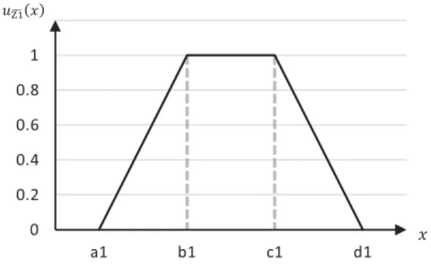
Definition 1: A trapezoidal fuzzy number ~z1can be represented as a quadruplet of real numbers (a1, b1, c1, d1) as shown
in Figure1.
Definition 2: Given two fuzzy trapezoidal fuzzy numbers ~z1= (a1, b1, c1, d1) and ~z2= (a2, b2, c2, d2) and any positive
real number r, the main operations on fuzzy numbers can be defined as follows (Chen, Lin, and Huang 2006):
~z1 ! ~z2¼ ða1þ a2; b1þ b2; c1þ c2; d1þ d2Þ (1)
~z1 Hez2¼ ða1& d2; b1& c2; c1& b2; d1& a2Þ (2)
~z1' ~z2¼ ða1( a2; b1( b2; c1( c2; d1( d2Þ (3)
~z1' r ¼ ða1( r; b1( r; c1( r; d1( rÞ (4)
Definition 3: Let ~z1= (a1, b1, c1, d1) and ~z2= (a2, b2, c2, d2) be two trapezoidal fuzzy numbers; the distance between
them can be calculated using the vertex method (Chen2000; Chen, Lin, and Huang2006):
Dð~z1; ~z2Þ ¼ ffiffiffiffiffiffiffiffiffiffiffiffiffiffiffiffiffiffiffiffiffiffiffiffiffiffiffiffiffiffiffiffiffiffiffiffiffiffiffiffiffiffiffiffiffiffiffiffiffiffiffiffiffiffiffiffiffiffiffiffiffiffiffiffiffiffiffiffiffiffiffiffiffiffiffiffiffiffiffiffiffiffiffiffiffiffiffiffiffiffiffiffiffiffiffiffiffi 1 4½ að 1& a2Þ 2þ b 1& b2 ð Þ2þ cð 1& c2Þ2þ dð 1& d2Þ2* r (5)
Definition 4: A matrix eD is called a fuzzy matrix if it includes at least a fuzzy entry (Buckley1985).
Definition 5: A linguistic variable is a variable which value is presented in linguistic terms (Zimmermann 2011).
Linguistic variables are commonly used to express subjective or qualitative appreciation of a decision-maker, using terms such as ‘very low’, ‘low’, ‘medium’, ‘high’, etc. Linguistic values can be modelled by fuzzy numbers.
4.3 From TOPSIS to Fuzzy TOPSIS
To compare solutions, TOPSIS computes the distance from each alternative to the Positive Ideal Solution (PIS) and Negative Ideal Solution (NIS). The PIS (resp. NIS) is the solution that minimises (resp. maximises) the ‘cost’ criteria and maximises (resp. minimises) the ‘benefit’ criteria (‘cost’ and ‘benefit’ are considered here in a broad sense). Fuzzy
TOPSIS uses linguistic variables to model the ratings and the weights of the criteria (Triantaphyllou and Lin1996; Chen
2000). This approach includes six steps:
Step 1: Construction of the fuzzy decisions matrix and of the weight vector
Let us assume that there are m possible alternatives Aiði¼ 1; . . .; mÞ to solve a problem, evaluated on n criteria
Cjðj¼ 1; . . .; nÞ. The rating of the alternatives with respect to the different criteria may be represented by a decision
matrix ~D:
e D¼ C1 C2 . . . Cn A1 ~x11 ~x12 . . . ~x1n A2 ~x21 ~x22 ~x2n . . . . Am ~xm1 ~xm2 . . . ~xmn (6)
where ~xijis a linguistic value that represents the performance rating of alternative Aiwith respect to criterion Cj.
The criteria weights can be expressed in a vector as follows: ~
w¼ ½~w1; ~w2; . . .; ~wn* (7)
where ~wj may also be a linguistic value that represents the importance weight of criterion j.
In this article, ~xij and ~wj (i = 1, …, m and j = 1, …, n) are assumed to be trapezoidal fuzzy numbers given by:
~
xij= (aij, bij, cij, dij) and ~wj= (w1j, w2j, w3j, w4j).
Step 2: Construction of the normalised fuzzy decisions matrix
The decision matrix is normalised to avoid anomalies resulting from different criteria scales. The set of criteria can be categorised into ‘cost’ criteria (Co) (to be minimised) and ‘benefit’ criteria (B) (to be maximised). The normalised fuzzy decision matrix can then be calculated as:
~ R¼ ½~rij*m(n; i¼ 1; . . .; m and j ¼ 1; . . .; n (8) ~rij¼ aij dþj ; bij dþj ; cij dþj ; dij dþj ! ; j2 B (9) ~ rij¼ a&j dij ;a & j cij ;a & j bij ;a & j aij & ' ; j2 Co (10)
where dþj = max_idijif j ∊ B and a&j = min_iaij, j ∊ Co.
Step 3: Construction of the weighted normalised fuzzy decisions matrix
The weighted normalised fuzzy decisions matrix is defined by multiplying the normalised fuzzy decision matrix by the importance weights of the criteria as follows:
~
V ¼ ½~vij*m(n; i¼ 1; 2; . . .; m; j¼ 1; 2; . . .; n (11)
~vij¼ ~rij' ~wj (12)
Step 4: Computation of the fuzzy positive ideal solution and the fuzzy negative ideal solution
The fuzzy positive ideal solution (FPIS) denoted by Aþ and the fuzzy negative ideal solution (FNIS) A−can be defined,
respectively, as: Aþ¼ ðevþ1;ev þ 2; . . .;ev þ nÞ (13) A&¼ ðev& 1;ev & 2; . . .;ev & nÞ (14) whereevþ
j = max_ievij4;ev&j = min_ievij1; i¼ 1; . . .; m; j = 1, …, n.
It should be noted that if all the criteria are assessed using the same set of fuzzy linguistic variables, there is no need to normalise the fuzzy decision matrix, and the FPIS and FNIS can be respectively defined as:
Aþ¼ ðevþ1;ev þ 2; . . .;ev
þ
nÞ ¼ ðmax_iVij4j j 2 BÞ; ðmin_iVij1j j 2 CoÞ (15)
A&¼ ðev&1;ev & 2; . . .;ev
&
Step 5: Determination of the distance between each alternative, FPIS and FNIS The distance from each alternative to the FPIS and the FNIS are:
diþ¼X n j¼1 dðevij;evþjÞ; i¼ 1; . . .; m (17) di&¼X n j¼1 dðevij;ev&jÞ; i¼ 1; . . .; m (18)
where d(·,·) denotes the distance between two fuzzy numbers, calculated using Equation (5). Step 6: Computation of the closeness coefficient and ranking the alternatives
In order to aggregate the two distances, a Closeness Coefficient (CC) is calculated for each alternative according to d+
and d−as follows: CCi¼ d&i d& i þ diþ ; i¼ 1; . . .; m (19)
CC is defined so that an alternative is close to FPIS and far from FNIS if its closeness coefficient is close to 1. We shall see in the next section how these methods and tools may be used to address the considered problem.
5. Problem description
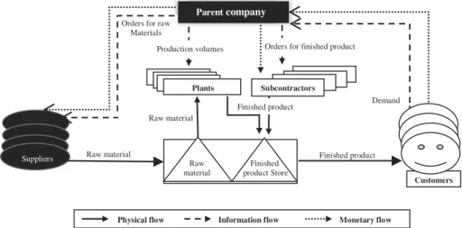
The structure of the SC considered in this work is presented in Figure2. This generic yet simplified SC is composed of
multiple suppliers, multiple parallel manufacturing plants and multiple subcontractors. Each manufacturing plant can produce several finished products using components provided by the suppliers. Production cost of the same product can be different according to the manufacturing plant. To increase its production capacity, each manufacturing plant can use overtime. Regular hours and overtime hours are limited for each period. For simplicity, we have not considered the transportation costs in this work (they can be considered as included in the costs of products, or can be added in a more precise way in the models if needed). In addition, it is assumed that the production durations are negligible. Again, tak-ing into account different production durations complicates the problem without setttak-ing specific theoretical issues. Costs and capacities of each supplier and subcontractor can be different.
We assume that a predefined list of approved suppliers is given. For simplification purpose, it is assumed that a manufacturing plant is considered as a single stage production system, for instance by considering the bottleneck resource.
Finished product Demand Orders for raw
Materials Raw material Raw material Customers Parentcompany Raw material Plants
Production volumes Orders for finished product
Finished product
Finished product Store
Physical flow Information flow Monetary flow
Suppliers
Subcontractors
6. Proposed approach 6.1 Notation • Set of indices: • Crisp parameters: • Fuzzy parameters: • Decision variables:
6.2 Presentation of the proposed approach The suggested approach consists of six main steps.
• Step 1: Select the criteria used for order allocation
In this first step, the decision-maker must choose among Class I and Class II criteria the ones that match with his strategy, or may add other criteria.
• Step 2: Provide the set of scenarios allowing to satisfy demand requirements We note:
Cp;t: a set of scenario able to satisfy demand requirements Dp;t
i: index of allocation scenario (i = 1, …, card (Cp;t)) where:
g
c rm;p;t Production cost for a unit of product p in regular time at manufacturing plant m in period t
g
c ovm;p;t Production cost for a unit of product p in overtime at manufacturing plant m in period t
g
c bb;p;t Subcontracting cost for a unit of product p by subcontractor b in period t
gc ss;r;t Purchasing cost of a unit of raw material r at supplier s in period t
g
Q mm, gQ bb; gQ ss Linguistic evaluation of quality related, respectively, to manufacturing plant m, to subcontractor b and to supplier s
g
Rl mm, gRl bb; gRl ss Linguistic evaluation of the reliability, respectively, related to manufacturing plant m, to subcontractor b and
to supplier s g
F mm, gF bb; gF ss Linguistic evaluation of the flexibility related, respectively, to manufacturing plant m, to subcontractor b and
to supplier s g
Rsp mm, g
Rsp bb; gRsp ss
Linguistic evaluation of the responsiveness related, respectively, to manufacturing plant m, to subcontractor b and to supplier s
g Rsi mm,
g
Rsi bb; gRsi ss
Linguistic evaluation of the resilience related, respectively, to manufacturing plant m, to subcontractor b and to supplier s
g Rob mm,
g
Rob bb; gRob ss
Linguistic evaluation of the robustness related, respectively, to manufacturing plant m, to subcontractor b and to supplier s
T Number of time periods (t = 1, …, T) P Number of finished products (p = 1, …, P) R Number of raw materials (r = 1, …, R) M Number of manufacturing plants (m = 1 ,…, M) S Number of suppliers (s = 1, …, S)
B Number of subcontractors (b = 1, …, B)
Sr Set of suppliers providing raw material r (i.e. Sr-{1,…,S})
Mp Set of manufacturing plants producing finished product p (i.e. Mp⊆ {1, …, M}) Bp Set of subcontractors supplying finished product p (i.e. Bp-{1, …, B})
Rp Set of raw materials required to produce a final product p
αp,r Quantity of raw material r required to produce a unit of final product p
cap rm;p;t Maximum number of product p that can be produced in regular time at manufacturing plant m during period t
cap ovm;p;t Maximum number of product p that can be produced in overtime at manufacturing plant m during period t
cap bb;p;t Maximum number of product p that can be provided by subcontractor b during period t
cap ss;r;t Maximum number of raw material r that can be provided by supplier s during period t
Dp,t Global demand of finished product p in period t resulting from all the customers
x rm;p;t Production quantity in regular time for product p at plant m in period t
x ovm;p;t Production quantity in overtime for product p at plant m in period t
x bb;p;t Subcontracting quantity for product p at subcontractor b in period t
Cp;t¼ fSip;tg ¼ fðx r i m;p;tÞm2MP;ðx ovim;p;tÞm2MP;ðx bb;p;ti Þb2BP;ðx Sim;p;tÞm2MPj ð21Þ–ð27 Þg (20) X m2MP x rm;p;ti þ X m2MP x ovim;p;tþ X b2BP x bib;p;t¼ Dp;t 8i; p; t (21) X s2Sr x sis;r;t¼ ðX m2MP x rim;p;tþ X m2MP x ovim;p;tÞ ( ap;r 8r 2 Rp; 8i; t (22) x rim;p;t1 cap rm;p;t 8i; m; p; t (23) x ovim;p;t1 cap ovm;p;t 8i; m; p; t (24) x bib;p;t1 cap bb;p;t 8i; b; p; t (25) x sis;r;t1 cap ss;r;t 8i; r; s; t (26) x rim;p;t; x ovim;p;t; x bib;p;t; x sis;r;t2 0 8i; p; r; t; m; b; s (27) Constraint (21) ensures that all customer demands are satisfied at the end of each planning period.
The quantity of each raw material to be supplied in each planning period is calculated using constraint (22). Con-straints (23) and (24) represent the manufacturer’s production capacity limitation during, respectively, regular and over-time hours.
Constraints (25) and (26) indicate the maximum utilised capacities at each supplier and subcontractor in each period, respectively.
Constraint (27) expresses the non-negativity of different decision variables. • Step 3: Evaluate the performance of each allocation scenario
(a) Rate each actor with respect to Class I criteria
The cost is given by a trapezoidal fuzzy number, whereas the quality and the reliability are supposed to be evaluated by the decision-maker using linguistic labels, according to previous experiences with the partner.
(b) Construct the fuzzy comparison matrix (allocation scenarios-selected criteria of Class I)
Using the results of step 3(a), the fuzzy comparison matrix can be constructed according to the Class I criteria defined in the first step, using the following proposals:
(i) The cost measure of each allocation scenario is the sum of production costs, supply costs and subcontracting
cots. If fTCip;t denotes the total cost measure of scenario Si
p;t, then: f TCip;t¼ X m2MP x rim;p;t'gc rm;p;t! X m2MP x ovim;p;t'c ovgm;p;t! X b2BP x bib;p;t' gc bb;p;t! X s2Sr X r2Rp x sis;r;t'gc ss;r;t 8i; p; t (28) (ii) The measure of each allocation scenario according to the criterion ‘number of actors’ can be evaluated by
calcu-lating the number of manufacturing sites, subcontractors and suppliers involved in this allocation. If nbi
p;tdenotes the number of actors related of scenario Sip;t then:
nbip;t¼ cardðEm;p;ti Þ 8i; p; t (29)
where
Em;p;ti ¼ fm 2 MPjx ri
We have now to aggregate the quality and reliability of the suppliers used in each considered scenario. We denote by e
Qip;t, eRlip;t, respectively, the quality and reliability measures associated to allocation scenario Sp;ti .
The assessment of each allocation according to the quality (resp. reliability) criterion can be estimated using various strategies. We limit our discussion to three classical ones, rather intuitive:
• Pessimistic strategy: The quality (resp. reliability) measure associated to an allocation scenario is assumed to be the quality (resp. reliability) of the worst partner:
~
Qip;t¼ MinðMinm2Ei
m;p;tQ mgm;p; Minb2Eim;p;tQ bgb;p; Mins2Eim;p;tQ sgs;rÞ 8i (31) e
Rlp;ti ¼ MinðMinm2Ei
m;p;tRl mg m;p; Minb2Eim;p;tRl bgb;p; Mins2Eim;p;tRl sgs;rÞ 8i (32)
• Optimistic strategy: The quality (resp. reliability) measure associated to an allocation scenario is assumed to be the quality (resp. reliability) of the best partner:
e Qip;t¼ Maxð Max m2Ei m;p;t g Q mm;p; Max b2Ei m;p;t g Q bb;p; Max s2Ei m;p;t g Q ss;rÞ 8i (33) e Rlip;t¼ Maxð Max m2Ei m;p;t g Rl mm;p; Max b2Ei m;p;t g Rl bb;p; Max b2Ei m;p;t g Rl ss;rÞ 8i (34)
• Medium strategy: The quality (resp. reliability) measure associated to an allocation scenario is assumed to be the average of the quality (resp. reliability) measures of the actors involved in this allocation scenario:
~ Qip;t¼ X m2MP ðx ri m;p;tþ x ovim;p;tÞ ' gQ mm;p ! ! X b2BP x bib;p;t' gQ bb;p ! ! X s2Sr X r2Rp x sis;r;t' gQ ss;r ! " # = X m2MP ðx ri m;p;tþ x ovim;p;tÞ þ X b2BP x bib;p;tþX s2Sr X r2Rp x sis;r;t ! " # (35) e Rlip;t¼ X m2MP ðx ri m;p;tþ x ovim;p;tÞ ' eRlm;p ! ! X b2BP x bib;p;t' fRlb;p ! ! ðX s2Sr X r2Rp x sis;r;t' fRls;rÞ " # = X m2MP ðx ri m;p;tþ x ovim;p;tÞ þ X b2BP x bib;p;tþX s2Sr X r2Rp x sis;r;t ! " # (36)
(c) Use of fuzzy TOPSIS
In this step, we apply the fuzzy TOPSIS method, considering the fuzzy decision matrix described in 3(b) and the
Class I criteria defined in the first step. At the end of this step, we can determine for each allocation scenario Si
p;t the
closeness coefficient CC Ii
p;t.
• Step 4: Evaluate the risk of each allocation scenario
(a) Measure the rating of each actor with respect to Class II criteria
We assume that the decision-maker provides in a linguistic form the rating of each actor with respect to the criteria of flexibility, responsiveness, resilience and robustness. Concerning the stability criterion, we assume that we have access to accurate information on the load of the actor during the previous period.
(b) Construct the fuzzy comparison matrix (allocation scenarios-Class II criteria)
The fuzzy decision matrix can be constructed according to the Class II criteria using the result of the previous step 5(a). The rating of each allocation scenario with respect to the criteria of Class II can be calculated according to the decision-maker strategy (i.e. optimistic strategy, pessimistic strategy or medium strategy) as described previously.
(c) Use of fuzzy TOPSIS
Fuzzy TOPSIS is then used, taking as an input the fuzzy decision matrix obtained in previous step. The method cal-culates the closeness coefficient of each allocation scenario according to the selected criteria related to Class II.
Obvi-ously, the allocation scenario with the highest closeness coefficient value CC IIi
p;twill be the less risky.
• Step 5: Interpretation of the results
The use of fuzzy TOPSIS has for outputs the two closeness coefficients related to Class I (performance) and Class
II (risk) criteria. Their interpretation can be facilitated by using rules such as those suggested in Table 1. The
perfor-mance is here rated according to the {do not recommend, recommend, approve} scale, while the risk is denoted by the {low, moderate, high} linguistic scale. The decision-maker can of course use other linguistic values to rate the allocation scenarios according to his strategy.
7. Numerical example
In this section, a numerical example is presented to show the applicability of the suggested approach. The main purpose of this example is to compare in a considered period t the performance and risk of different allocation scenarios that
satisfy the global demand of finished product p Dp;t= 28.
The case study involves two manufacturing plants (m = 1, 2) and two subcontractors (b = 1, 2) who produce the finished product p. One unit of raw material r is required to produce one unit of p. Each raw material r can be provided
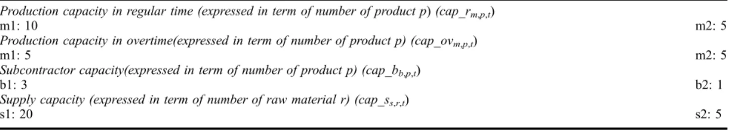
by two suppliers (s = 1, 2). Data on the capacities of the considered SC are given in Table2.
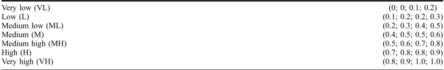
The decision-maker uses the classical linguistic variables presented in Table 3 to assess the importance of the
various criteria. The linguistic variables shown in Table4 (also classical) are used to rate the actors with respect to each
criterion (Hatami-Marbini and Tavana2011).
Table 1. Proposed rules of assessment status of Sp;ti . Closeness coefficient CC Ii
p;t Closeness coefficient CC IIp;ti Assessment status of Sp;ti
CC Ii
p;t2 [0, 0.4) 8CC IIp;ti Do not recommend
CC Ii
p;t2 [0.4, 0.75) CC IIp;ti 2 [0, 0.4) Recommend with high risk
CC IIp;ti 2 [0.4, 0.75) Recommend with moderate risk CC IIp;ti 2 [0.75, 1] Recommend with low risk CC Ii
p;t2 [0.75, 1] CC IIp;ti 2 [0, 0.4) Approved with high risk
CC IIi
p;t2 [0.4, 0.75) Approved with moderate risk
CC IIi
p;t2 [0.75, 1] Approved and preferred
Table 2. Capacity data for the supply chain network.
Production capacity in regular time (expressed in term of number of product p) (cap_rm,p,t)
m1: 10 m2: 5
Production capacity in overtime(expressed in term of number of product p) (cap_ovm,p,t)
m1: 5 m2: 5
Subcontractor capacity(expressed in term of number of product p) (cap_bb,p,t)
b1: 3 b2: 1
Supply capacity (expressed in term of number of raw material r) (cap_ss,r,t)
The computational procedure can be summarised as follows: Step 1: Select the used criteria for order allocation
The decision-maker chooses for instance the following criteria: • Class I: Performance strategy and quality of service
(1) Cost (2) Quality (3) Reliability (4) Number of actors • Class II: Risk
(1) Flexibility (2) Responsiveness (3) Resilience (4) Robustness (5) Stability
Step 2: Provide the set of scenario able to satisfy demand requirements
In a preliminary study, the analytical model has been implemented in LINGO in order to get the optimal solution of
the problem when a simple objective function linked to cost is used (Khemiri et al. 2015). As a consequence, reusing
the LINGO model while removing the objective function allows easily generating all the possible scenarios satisfying
the demand (see Table5); the solver was therefore used for checking the satisfaction of the constraints.
Step 3: Evaluate the performance of each allocation scenario • Assess the rating of each actor with respect to Class I criteria
The ratings of the actors defined by the decision-maker according to the various criteria of Class I are shown in
Table 6. The cost ratings are given as trapezoidal fuzzy numbers while the quality and reliability ratings are given
through linguistic variables that can be converted into trapezoidal fuzzy numbers using Table4.
• Construct the fuzzy comparison matrix
We assume that the decision-maker uses the medium strategy to assess each allocation scenario on the quality and reliability criteria (formulae (35) and (36)). The cost measures are obtained using formula (28) and the number of actors
is given by formula (29). The result is the fuzzy decision matrix of Table 7.
Table 3. Linguistic variables for the importance weight of each criterion (Hatami-Marbini and Tavana2011).
Very low (VL) (0; 0; 0.1; 0.2) Low (L) (0.1; 0.2; 0.2; 0.3) Medium low (ML) (0.2; 0.3; 0.4; 0.5) Medium (M) (0.4; 0.5; 0.5; 0.6) Medium high (MH) (0.5; 0.6; 0.7; 0.8) High (H) (0.7; 0.8; 0.8; 0.9) Very high (VH) (0.8; 0.9; 1.0; 1.0)
Table 4. Linguistic variables for ratings (Hatami-Marbini and Tavana2011).
Very poor (VP) (0; 0; 1; 2) Poor (P) (1; 2; 2; 3) Medium poor (MP) (2; 3; 4; 5) Fair (F) (4; 5; 5; 6) Medium good (MG) (5; 6; 7; 8) Good (G) (7; 8; 8; 9) Very good (VG) (8; 9; 10; 10)
• Use of Fuzzy TOPSIS
Fuzzy TOPSIS is used with as input the fuzzy decision matrix shown in Table 7. The importance weights of the
Class I criteria determined by the decision-maker are shown in Table 8. Table 7 is used to obtain the normalised Fuzzy
decision matrix presented in Table 9 using the formulae (9) and (10). Using the normalised Fuzzy decision matrix and
the importance weights of the criteria in Table8, a weight normalised Fuzzy decision matrix is calculated using formula
(12), as shown in Table10.
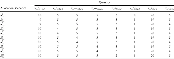
Table 5. The set of allocation scenarios.
Allocation scenarios Quantity x_rm1,p,t x_rm2,p,t x_ovm1,p,t x_ovm2,p,t x_bb1,p,t x_bb2,p,t x_ss1,r,t x_ss2,r,t S1 p;t 10 5 5 5 3 0 20 5 S2 p;t 9 5 5 5 3 1 19 5 S3 p;t 9 5 5 5 3 1 20 4 S4 p;t 10 4 5 5 3 1 19 5 S5 p;t 10 4 5 5 3 1 20 4 S6 p;t 10 5 4 5 3 1 19 5 Sp;t7 10 5 4 5 3 1 20 4 S8 p;t 10 5 5 4 3 1 19 5 S9 p;t 10 5 5 4 3 1 20 4 S10 p;t 10 5 5 5 2 1 20 5
Table 6. Ratings of the actors by the decision-maker using selected criteria of Class I.
Criteria Class I
Actors
m1 m2 b1 b2 s1 s2
Cost Regular time cost: Regular time cost: (45, 50, 50, 53) (250,260,265,270) (5,10,12,17) (10,15,20,25) (9, 10, 11, 12) (1, 2, 3, 5)
Overtime cost: Overtime cost: (26, 27,28,30) (15, 16, 17, 20)
Quality G VG MG P G VG
Reliability G VG G VP MG VG
Table 7. Fuzzy comparison matrix (allocation scenarios-Class I criteria).
Allocation scenarios
Criteria
Cost Quality Reliability Number of actors
S1 p;t (585, 750, 840, 1019) (7.169, 8.169,8.509,9.226) (6.528,7.528, 8.188, 8.905) (5,5,5,5) S2 p;t (821, 990, 1082,1260) (7.057,8.057, 8.403, 9.115) (6.423,7.403, 8.076, 8.788) (6,6,6,6) Sp;t3 (816, 985, 1074,1252) (7.038,8.038, 8.365, 9.096) (6.365,7.346, 8.019, 8.750) (6,6,6,6) S4 p;t (829, 998, 1090,1267) (7.038,8.038, 8.365, 9.096) (6.403,7.384, 8.038, 8.769) (6,6,6,6) S5 p;t (824, 993, 1082,1259) (7.019,8.019, 8.326, 9.076) (6.346,7.326, 7.980, 8.730) (6,6,6,6) S6 p;t (804, 973, 1065,1242) (7.057,8.057, 8.403, 9.115) (6.423,7.403, 8.076, 8.788) (6,6,6,6) S7 p;t (799, 968, 1057,1234) (7.038,8.038, 8.365, 9.096) (6.365,7.346, 8.019, 8.750) (6,6,6,6) S8 p;t (815, 984, 1076,1252) (7.038,8.038, 8.365, 9.096) (6.403,7.384, 8.038, 8.769) (6,6,6,6) S9 p;t (810, 979, 1068,1244) (7.019,8.019, 8.326, 9.076) (6.346,7.326, 7.980, 8.730) (6,6,6,6) S10 p;t (790, 960, 1055,1236) (7.094,8.094, 8.415, 9.132) (6.396,7.377, 8.056, 8.773) (6,6,6,6)
The fuzzy positive ideal solution (Aþ) and the FNIS (A&) (which are crisp numbers) are calculated using formulae (13) and (14) as follows:
Aþ¼ ½ð1; 1; 1; 1Þ; ð0:6; 0:6; 0:6; 0:6Þ; ð0:9; 0:9; 0:9; 0:9Þ; ð1; 1; 1; 1Þ*
A&¼ ½ð0:369; 0:369; 0:369; 0:369Þ; ð0:304; 0:304; 0:304; 0:304Þ; ð0:498; 0:498; 0:498; 0:498Þ; ð0:666; 0:666; 0:666; 0:666Þ*
The distance of each allocation scenario Si
p;t to A
+
and A− with respect to the various criteria is calculated using formula
(5), as shown, respectively, in Tables11and12.
The calculated diþand d&i of the various allocation scenarios Si
p;tcan, respectively, be obtained using formulae (17) and
(18) as shown in Table13. The closeness coefficient of the allocation scenarios is then calculated using formula (19).
Step 4: Evaluate the risk of each allocation scenario
• Measure the rating of each partner with respect to Class II criteria
The ratings of the actors defined by the decision-maker according to the criteria of Class II are shown in Table14.
The flexibility, responsiveness, resilience and robustness ratings are given using linguistic variables. For the criterion of stability, the decision-maker knows the previous load of each actor; the instability measurement is determined by calcu-lating the difference between the previous and the actual load.
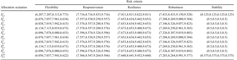
• Construct the fuzzy comparison matrix (allocation scenarios - risk criteria)
We assume that the decision-maker uses the ‘average’ strategy to calculate the measure of each allocation scenario
according to the risk criteria. The result is given in Table 15.
rch Table 8. Importance weights of Class I criteria.
Criteria I
Cost Quality Reliability Number of actors
VH M H VH
Table 9. Normalised fuzzy decision matrix – Class I.
Allocation scenarios
Criteria I
Cost Quality Reliability Number of actors
S1 p;t (0.574, 0.696, 0.780,1) (0.777, 0.885, 0.922, 1) (0.733, 0.845, 0.919, 1) (1, 1, 1, 1) S2 p;t (0.464,0.540, 0.590,0.712) (0.764,0.873, 0.910,0.987) (0.721,0.831, 0.906, 0.986) (0.833, 0.833, 0.833, 0.833) S3 p;t (0.467,0.544, 0.593,0.716) (0.762,0.871, 0.906,0.985) (0.714,0.824, 0.900, 0.982) (0.833, 0.833, 0.833, 0.833) S4 p;t (0.461,0.536, 0.586,0.705) (0.762,0.871, 0.906,0.985) (0.719,0.829, 0.902, 0.984) (0.833, 0.833, 0.833, 0.833) S5 p;t (0.464,0.540, 0.589,0.709) (0.760,0.869, 0.902,0.983) (0.712,0.822, 0.896, 0.980) (0.833, 0.833, 0.833, 0.833) S6 p;t (0.471,0.549, 0.601, 0.727) (0.764,0.873, 0.910,0.987) (0.721,0.831, 0.906, 0.986) (0.833, 0.833, 0.833, 0.833) S7 p;t (0.474,0.553, 0.604, 0.732) (0.762,0.871, 0.906,0.985) (0.714,0.824, 0.900, 0.982) (0.833, 0.833, 0.833, 0.833) S8 p;t (0.467,0.543, 0.594, 0.717) (0.762,0.871, 0.906,0.985) (0.719,0.829, 0.902, 0.984) (0.833, 0.833, 0.833, 0.833) S9 p;t (0.470,0.547, 0.597, 0.722) (0.760,0.869, 0.902,0.983) (0.712,0.822, 0.896, 0.980) (0.833, 0.833, 0.833, 0.833) S10 p;t (0.473,0.554, 0.609, 0.740) (0.768,0.877, 0.912,0.989) (0.718,0.828, 0.904, 0.985) (0.833, 0.833, 0.833, 0.833)
Table 10. Weighted normalised fuzzy decision matrix – Class I
Allocation Scenarios
Criteria
Cost Quality Reliability Number of actors
S1 p;t (0.459, 0.626, 0.780, 1) (0.310, 0.442, 0.461, 0.6) (0.513, 0.676, 0.735, 0.9) (0.8, 0.9, 1, 1) S2 p;t (0.371, 0.486, 0.590, 0.712) (0.305, 0.436, 0.455, 0.592) (0.504, 0.665, 0.725, 0.888) (0.666, 0.750, 0.833, 0.833) S3 p;t (0.373, 0.490, 0.593, 0.716) (0.305, 0.435, 0.453, 0.591) (0.500, 0.659, 0.720, 0.884) (0.666, 0.750, 0.833, 0.833) S4 p;t (0.369, 0.483, 0.586, 0.705) (0.305, 0.435, 0.453, 0.591) (0.503, 0.663, 0.722, 0.886) (0.666, 0.750, 0.833, 0.833) S5 p;t (0.371, 0.486, 0.589, 0.709) (0.304, 0.434, 0.451, 0.590) (0.498, 0.658, 0.716, 0.882) (0.666, 0.750, 0.833, 0.833) S6 p;t (0.376, 0.494, 0.601, 0.727) (0.305, 0.436, 0.455, 0.592) (0.504, 0.665, 0.725, 0.888) (0.666, 0.750, 0.833, 0.833) S7 p;t (0.379, 0.498, 0.604, 0.732) (0.305, 0.435, 0.453, 0.591) (0.500, 0.659, 0.720, 0.884) (0.666, 0.750, 0.833, 0.833) S8 p;t (0.373, 0.489, 0.594, 0.717) (0.305, 0.435, 0.453, 0.591) (0.503, 0.663, 0.722, 0.886) (0.666, 0.750, 0.833, 0.833) S9 p;t (0.376, 0.492, 0.597, 0.722) (0.304, 0.434, 0.451, 0.590) (0.498, 0.658, 0.716, 0.882) (0.666, 0.750, 0.833, 0.833) S10 p;t (0.378, 0.499, 0.609, 0.740) (0.307, 0.438, 0.456, 0.593) (0.502, 0.662, 0.723, 0.886) (0.666, 0.750, 0.833, 0.833)
Table 11. Distance between each allocation scenario and Aþ.
Allocation scenarios
Criteria
Cost Quality Reliability Number of actors
S1 p;t 0.3464 0.1786 0.2380 0.1118 S2 p;t 0.4766 0.1830 0.2459 0.2393 S3 p;t 0.4735 0.1840 0.2499 0.2393 S4 p;t 0.4803 0.1840 0.2475 0.2393 S5 p;t 0.4772 0.1850 0.2516 0.2393 Sp;t6 0.4683 0.1830 0.2459 0.2393 S7 p;t 0.4651 0.1840 0.2499 0.2393 S8 p;t 0.4735 0.1840 0.2475 0.2393 S9 p;t 0.4704 0.1850 0.2516 0.2393 S10 p;t 0.4628 0.1818 0.2476 0.2393
• Use of fuzzy TOPSIS
• The decision-maker provides the weights of the risk criteria shown in Table16. This table and the fuzzy decision
matrix presented in Table 15 are used for calculating the closeness coefficient for each allocation scenario as
shown in Table17.
Step 5: Interpretation of the results
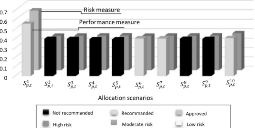
The rules presented in Table1 have been used to classify the allocation scenarios in Figure3. As seen in Figure3, the
first scenario S1
p;t denotes better performance and risk measures than the other solutions, and is ‘recommended’ with
rch Table 12. Distance between each allocation scenario and A&.
Allocation scenarios
Criteria
Cost Quality Reliability Number of actors
S1 p;t 0.4001 0.1811 0.2493 0.2713 S2 p;t 0.2124 0.1757 0.2401 0.1250 S3 p;t 0.2155 0.1746 0.2364 0.1250 S4 p;t 0.2079 0.1746 0.2382 0.1250 S5 p;t 0.2109 0.1734 0.2345 0.1250 S6 p;t 0.2223 0.1757 0.2401 0.1250 Sp;t7 0.2255 0.1746 0.2364 0.1250 S8 p;t 0.2159 0.1746 0.2382 0.1250 S9 p;t 0.2190 0.1734 0.2345 0.1250 S10 p;t 0.2303 0.1767 0.2386 0.1250
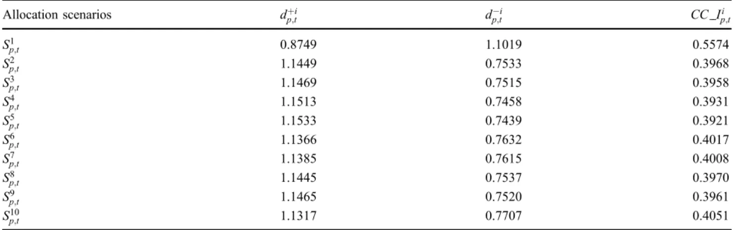
Table 13. Computation of dþip;t, dp;t&i;jand CC Ip;ti .
Allocation scenarios dþi
p;t dp;t&i CC Ip;ti Sp;t1 0.8749 1.1019 0.5574 S2 p;t 1.1449 0.7533 0.3968 S3 p;t 1.1469 0.7515 0.3958 S4 p;t 1.1513 0.7458 0.3931 S5 p;t 1.1533 0.7439 0.3921 Sp;t6 1.1366 0.7632 0.4017 S7 p;t 1.1385 0.7615 0.4008 S8 p;t 1.1445 0.7537 0.3970 S9 p;t 1.1465 0.7520 0.3961 S10 p;t 1.1317 0.7707 0.4051
Table 14. Ratings of the actors by the decision-maker under Class II criteria.
Criteria Class B Actors m1 m2 b1 b2 s1 s2 Flexibility VG MG VG VP MG G Responsiveness VG G VG VP VG G Resilience VG G VG VP VG VG Robustness G VG VG VP VG MG
Stability (Previous load) x rm1;p;t&1¼ 11 x rm2;p;t&1¼ 5 3 0 20 5
Table 15. Fuzzy comparison matrix (allocation scenarios-Class II criteria).
Allocation scenarios
Risk criteria
Flexibility Responsiveness Resilience Robustness Stability
S1 p;t (6.207,7.207,8.113,8.773) (7.716,8.716,9.433,9.716) (7.811,8.811,9.622,9.811) (7.433,8.433,9.150,9.528) (0.125,0.125,0.125,0.125) S2 p;t (6.076,7.057,7.961,8.634) (7.557,8.538,9.250,9.557) (7.653,8.634,9.442,9.653) (7.288,8.269,9.000,9.384) (0.5,0.5,0.5,0.5) S3 p;t (6.038,7.019,7.942,8.615) (7.576,8.557,9.288,9.576) (7.653,8.634,9.442,9.653) (7.346,8.326,9.057,9.423) (0.5,0.5,0.5,0.5) S4 p;t (6.134,7.115,8.019,8.673) (7.576,8.557,9.288,9.576) (7.673,8.653,9.480,9.673) (7.269,8.250,8.961,9.365) (0.5,0.5,0.5,0.5) S5 p;t (6.096,7.076,8.000,8.653) (7.596,8.576,9.326,9.596) (7.673,8.653,9.480,9.673) (7.326,8.307,9.019,9.403) (0.5,0.5,0.5,0.5) S6 p;t (6.076,7.057,7.961,8.634) (7.557,8.538,9.250,9.557) (7.653,8.634,9.442,9.653) (7.288,8.269,9.000,9.384) (0.5,0.5,0.5,0.5) S7 p;t (6.038,7.019,7.942,8.615) (7.576,8.557,9.288,9.576) (7.653,8.634,9.442,9.653) (7.346,8.326,9.057,9.423) (0.5,0.5,0.5,0.5) S8 p;t (6.134,7.115,8.019,8.673) (7.576,8.557,9.288,9.576) (7.673,8.653,9.480,9.673) (7.269,8.250,8.961,9.365) (0.5,0.5,0.5,0.5) S9 p;t (6.096,7.076,8.000,8.653) (7.596,8.576,9.326,9.596) (7.673,8.653,9.480,9.673) (7.326,8.307,9.019,9.403) (0.5,0.5,0.5,0.5) S10 p;t (6.056,7.037,7.943,8.622) (7.566,8.547,9.264,9.566) (7.660,8.641,9.452,9.660) (7.283,8.264,8.981,9.377) (0.375,0.375,0.375,0.375)
rch Table 16. Importance weights of Class II criteria.
Criteria B
Flexibility Responsiveness Resilience Robustness Stability
VH H H VH VH Table 17. Computation of CC IIi p;t. Allocation scenarios CC IIi p;t S1 p;t 0.6367 S2 p;t 0.3679 S3 p;t 0.3692 S4 p;t 0.3700 S5 p;t 0.3713 S6 p;t 0.3679 S7 p;t 0.3692 S8 p;t 0.3700 S9 p;t 0.3713 S10 p;t 0.3950
Table 18. Experiments for sensibility analysis.
Expt. no.
Definition
Importance weights of Class I criteria Importance weights of Class II criteria
Cost Quality Reliability Number of actors Flexibility Responsiveness Resilience Robustness Stability
1 VL VL VL VL VL VL VL VL VL 2 M M M M M M M M M 3 VH VH VH VH VH VH VH VH VH 4 VH VL VL VL VL VL VL VL VL 5 VL VH VL VL VL VL VL VL VL 6 VL VL VH VL VL VL VL VL VL 7 VL VL VL VH VL VL VL VL VL 8 VL VL VL VL VH VL VL VL VL 9 VL VL VL VL VL VH VL VL VL 10 VL VL VL VL VL VL VH VL VL 11 VL VL VL VL VL VL VL VH VL 12 VL VL VL VL VL VL VL VL VH 13 VH VH VH VH VL VL VL VL VL 14 VL VL VL VL VH VH VH VH VH 15 VL L ML M MH H VH VH VL 16 VH H MH M ML L VL VL VH 17 H ML M MH L VL VH H ML 18 ML MH VH VL L M H H M
Table 19. Results of sensibility analysis: performance measure. Expt.no. CC Iip;t Ranking R1 R2 R3 R4 R5 R6 R7 R8 R9 R10 1 0.4199 0.3856 0.3854 0.3847 0.3844 0.3867 0.3865 0.3856 0.3854 0.3877 R1>R10>R6>R7>R8>R2>R9>R3>R4>R5 2 0.5203 0.4051 0.4039 0.4020 0.4008 0.4085 0.4073 0.4048 0.4036 0.4112 R1>R10>R6>R7>R2>R8>R3>R9>R4>R5 3 0.5729 0.4240 0.4224 0.4200 0.4183 0.4284 0.4269 0.4236 0.4220 0.4318 R1>R10>R6>R7>R2>R8>R3>R9>R4>R5 4 0.4781 0.3590 0.3607 0.3558 0.3575 0.3654 0.3672 0.3610 0.3627 0.3702 R1>R10>R7>R6>R9>R8>R3>R2>R5>R4 5 0.4699 0.4369 0.4352 0.4347 0.4330 0.4378 0.4361 0.4354 0.4338 0.4400 R1>R10>R6>R2>R7>R8>R3>R4>R9>R5 6 0.4714 0.4393 0.4359 0.4371 0.4337 0.4401 0.4368 0.4378 0.4344 0.4395 R1>R6>R10>R2>R8>R4>R7>R3>R9>R5 7 0.5129 0.3736 0.3734 0.3728 0.3726 0.3747 0.3745 0.3736 0.3734 0.3756 R1>R10>R6>R7>R8>R2>R9>R3>R4>R5 8 0.4199 0.3856 0.3854 0.3847 0.3844 0.3867 0.3865 0.3856 0.3854 0.3877 R1>R10>R6>R7>R8>R2>R9>R3>R4>R5 9 0.4199 0.3856 0.3854 0.3847 0.3844 0.3867 0.3865 0.3856 0.3854 0.3877 R1>R10>R6>R7>R8>R2>R9>R3>R4>R5 10 0.4199 0.3856 0.3854 0.3847 0.3844 0.3867 0.3865 0.3856 0.3854 0.3877 R1>R10>R6>R7>R8>R2>R9>R3>R4>R5 11 0.4199 0.3856 0.3854 0.3847 0.3844 0.3867 0.3865 0.3856 0.3854 0.3877 R1>R10>R6>R7>R8>R2>R9>R3>R4>R5 12 0.4199 0.3856 0.3854 0.3847 0.3844 0.3867 0.3865 0.3856 0.3854 0.3877 R1>R10>R6>R7>R8>R2>R9>R3>R4>R5 13 0.5729 0.4240 0.4224 0.4200 0.4183 0.4284 0.4269 0.4236 0.4220 0.4318 R1>R10>R6>R7>R2>R8>R3>R9>R4>R5 14 0.4199 0.3856 0.3854 0.3847 0.3844 0.3867 0.3865 0.3856 0.3854 0.3877 R1>R10>R6>R7>R8>R2>R9>R3>R4>R5 15 0.4999 0.4208 0.4194 0.4194 0.4180 0.4217 0.4203 0.4201 0.4187 0.4223 R1>R10>R6>R2>R7>R8>R3>R4>R9>R5 16 0.5304 0.4058 0.4049 0.4021 0.4011 0.4105 0.4097 0.4059 0.4050 0.4142 R1>R10>R6>R7>R8>R2>R9>R3>R4>R5 17 0.5215 0.3925 0.3922 0.3896 0.3892 0.3968 0.3966 0.3930 0.3928 0.3999 R1>R10>R6>R7>R8>R9>R2>R3>R4>R5 18 0.4984 0.4459 0.4433 0.4430 0.4403 0.4481 0.4455 0.4447 0.4421 0.4495 R1>R10>R6>R2>R7>R8>R3>R4>R9>R5
Table 20. Results of sensibility analysis: risk measure. Expt. no. CC IIip;t Ranking R1 R2 R3 R4 R5 R6 R7 R8 R9 R10 1 0.4245 0.3664 0.3667 0.3668 0.3671 0.3664 0.3667 0.3668 0.3671 0.3726 R1>R10>R9>R5>R8>R4>R7>R3>R6>R2 2 0.5847 0.3726 0.3737 0.3743 0.3754 0.3726 0.3737 0.3743 0.3754 0.3930 R1>R10>R9>R5>R8>R4>R7>R3>R6>R2 3 0.6565 0.3860 0.3873 0.3882 0.3895 0.3860 0.3873 0.3882 0.3895 0.4123 R1>R10>R9>R5>R8>R4>R7>R3>R6>R2 4 0.4245 0.3664 0.3667 0.3668 0.3671 0.3664 0.3667 0.3668 0.3671 0.3726 R1>R10>R9>R5>R8>R4>R7>R3>R6>R2 5 0.4245 0.3664 0.3667 0.3668 0.3671 0.3664 0.3667 0.3668 0.3671 0.3726 R1>R10>R9>R5>R8>R4>R7>R3>R6>R2 6 0.4245 0.3664 0.3667 0.3668 0.3671 0.3664 0.3667 0.3668 0.3671 0.3726 R1>R10>R9>R5>R8>R4>R7>R3>R6>R2 7 0.4245 0.3664 0.3667 0.3668 0.3671 0.3664 0.3667 0.3668 0.3671 0.3726 R1>R10>R9>R5>R8>R4>R7>R3>R6>R2 8 0.4795 0.3984 0.3974 0.4013 0.4002 0.3984 0.3974 0.4013 0.4002 0.4024 R1>R10>R8>R4>R9>R5>R6>R2>R7>R3 9 0.4700 0.4145 0.4159 0.4160 0.4174 0.4145 0.4159 0.4160 0.4174 0.4202 R1>R10>R9>R5>R8>R4>R7>R3>R6>R2 10 0.4709 0.4157 0.4159 0.4172 0.4174 0.4157 0.4159 0.4172 0.4174 0.4212 R1>R10>R9>R5>R8>R4>R7>R3>R6>R2 11 0.4694 0.4151 0.4179 0.4143 0.4171 0.4151 0.4179 0.4143 0.4171 0.4198 R1>R10>R7>R3>R9>R5>R6>R2>R8>R4 12 0.6215 0.2528 0.2531 0.2532 0.2534 0.2528 0.2531 0.2532 0.2534 0.2936 R1<R10<R9<R5<R8<R4<R7<R3<R6<R2 13 0.4245 0.3664 0.3667 0.3668 0.3671 0.3664 0.3667 0.3668 0.3671 0.3726 R1>R10>R9>R5>R8>R4>R7>R3>R6>R2 14 0.6565 0.3860 0.3873 0.3882 0.3895 0.3860 0.3873 0.3882 0.3895 0.4123 R1>R10>R9>R5>R8>R4>R7>R3>R6>R2 15 0.5320 0.4691 0.4710 0.4712 0.4731 0.4691 0.4710 0.4712 0.4731 0.4723 R1>R9>R5>R10>R8>R4>R7>R3>R6>R2 16 0.6287 0.2872 0.2872 0.2882 0.2882 0.2872 0.2872 0.2882 0.2882 0.3238 R1>R10>R9>R5>R8>R4>R7>R3>R6>R2 17 0.5461 0.3975 0.3992 0.3982 0.3999 0.3975 0.3992 0.3982 0.3999 0.4125 R1>R10>R9>R5>R7>R3>R8>R4>R6>R2 18 0.5838 0.3826 0.3847 0.3836 0.3857 0.3826 0.3847 0.3836 0.3857 0.4028 R1>R10>R9>R5>R7>R3>R8>R4>R6>R2
‘moderate risk’. The main reason is that this scenario implies fewer actors (5 actors instead of 6 in the other scenarios); moreover, subcontractor b2, who has a poor performance (high cost, poor quality and reliability) and a very low resis-tance to the risk factors (very poor flexibility, responsiveness, etc.) is not involved.
The scenarios S6p;t, Sp;t7 and Sp;t10 are recommended with high risk whereas all the other scenarios are not
recom-mended according to the rules suggested in Table1.
In our opinion, the results presented in Figure 3 may allow a decision-maker to determine a balanced solution
between expected performance and risk.
8. Sensitivity analysis
The use of overlapping fuzzy weights is known as giving some intrinsic robustness to the aggregation method. As an
illustration, a sensitivity analysis was conducted. The details of 18 experiments are summarised in Table 18. For
exam-ple, in thefirst three experiments, the weights of all decision criteria are assumed to be equal to ‘VL’, ‘M’ and ‘VH’. In
experiments 4–12, the importance weight of each decision criteria is assumed to be ‘Very High (VH)’ and the rest of the criteria are set to ‘Very Low (VL)’. In experiment 13 (resp. 14), the weights of all performance-based decision criteria (resp. risk-based decision criteria) are set to the highest value (VH), while weights of all risk-based decision cri-teria (resp. performance-based decision cricri-teria) are set as lowest value (VL). The remaining experiments were randomly generated.
The results of the sensitivity analysis are illustrated in Tables 19 and 20. It can be seen that, although the rank of
some allocation scenarios changes with respect to different fuzzy weight bases, Sp;t1 is still selected as the best allocation
scenario, since it has the highest performance and risk measures. We can also notice that out of 18 experiments, Sp;t10 has
the second rank in 17 experiments according to both performance and risk measures. Additionally, the allocation
sce-nario S5
p;t has the lowest performance score in all the experiments and Sp;t2 has the lowest risk score in 16 experiments.
Therefore, we can conclude that the proposed decision-making approach is relatively robust to small changes in the fuzzy criteria weights on this example.
9. Conclusion and future research work
Nowadays, most SC networks are affected by various sources of uncertainty, including an increased variability of the demand. Consequently, making explicit the risk linked to the future execution of a supply plan may be an asset for sup-porting the decision of the logistic managers. However, the academic literature still shows a lack of approaches consid-ering risk-based factors when constructing a procurement–production tactical plan. The existing studies are indeed mainly based on the optimisation of performance factors, and often focus on price or profit criteria.
This article proposes to use a multi-criteria decision-making approach to deal with an integrated procurement– production system in a multi-echelon SC network involving multiple suppliers, multiple production sites, multiple sub-contractors and several customers, in which some critical data are evaluated in an imprecise way using fuzzy logic. The decision-maker selects first risk-based and performance-based decision criteria that match his strategy and his industrial context. The set of possible plans is generated as well as their performance and risk measures, in order to better support the selection of a procurement–production plan.
The main interest of the proposal is in our opinion to keep a clear distinction between assessment criteria linked to performance and to risk, since there is clearly no ‘mechanical’ compensation between these types of criteria in real situ-ations
Another interest of the method is that it better preserves the decision maker’s preferences than existing optimisation approaches. Additionally, it provides appropriate flexibility to the decision-maker for selecting the preferred tactical plan among several alternatives. The developed approach is generic in nature and can be easily extended to other selection problems.
The suggested approach has of course limitations. Some of them are classical, like the possible interaction between the dispersion of the assessments and the weights of the criteria. Others are linked to the chosen strategy, i.e. the genera-tion of all the possible scenarios, which makes difficult to address very large/multi-period problems. Extensions of this work are in progress for defining heuristics in order to only generate a given number of ‘good’ scenarios. Other limita-tions are linked to the hypothesis considered for simplifying the problem: it would for instance be more realistic to incorporate several distribution centres in order to deal with an integrated procurement, production and distribution plan-ning problem. The method should also be extended to take into account the various lead times associated with purchas-ing and manufacturpurchas-ing. Additionally, we assumed for simplicity that the customer demand is deterministic: it would be interesting to consider it as uncertain. Addressing these limitations will be the next step of this study.