a publisher's https://oatao.univ-toulouse.fr/26921
https://doi.org/10.1029/2020JE006387
Kenda, Balthasar and Drilleau, Mélanie and Garcia, Raphaël F.,... [et al.] Subsurface Structure at the InSight Landing Site From Compliance Measurements by Seismic and Meteorological Experiments. (2020) Journal of Geophysical Research: Planets, 125 (6). 1-30. ISSN 2169-9097
meteorological experiments
3B. Kenda1, M. Drilleau1, R. F. Garcia2, T. Kawamura1, N. Murdoch2, N.
4
Compaire2, P. Lognonn´e1, A. Spiga3,4, R. Widmer-Schnidrig5, P. Delage6, V.
5
Ansan7, C. Vrettos8, S. Rodriguez1, W. B. Banerdt9, D. Banfield10, D.
6
Antonangeli11, U. Christensen12, D. Mimoun2, A. Mocquet7, T. Spohn13
7
1Universit´e de Paris, Institut de physique du globe de Paris, CNRS, F-75005 Paris, France
8
2Institut Sup´erieur de l’A´eronautique et de l’Espace ISAE-SUPAERO, 10 Avenue Edouard Belin, 31400
9
Toulouse, France
10
3Laboratoire de M´et´eorologie Dynamique / Institut Pierre-Simon Laplace (LMD/IPSL), Sorbonne
11
Universit´e, Centre National de la Recherche Scientifique (CNRS), ´Ecole Polytechnique, ´Ecole Normale
12
Sup´erieure (ENS)
13
4Institut Universitaire de France (IUF)
14
5Black Forest Observatory, Stuttgart University, Heubach 206, D-77709 Wolfach, Germany
15
6Ecole des Ponts ParisTech, Laboratoire Navier/CERMES, CNRS, F 77455 Marne la Vallee, France
16
7Laboratoire de Plan´etologie et G´eodynamique, UMR6112-CNRS, Univ. Nantes, Univ. Angers, 44322
17
Nantes Cedex 3, France
18
8Division of Soil Mechanics and Foundation Engineering, Technical University of Kaiserslautern, 67663
19
Kaiserslautern, Germany
20
9Jet Propulsion Laboratory, California Institute of Technology, Pasadena, CA 91109, USA
21
10Cornell University, Cornell Center for Astrophysics and Planetary Science, Ithaca, NY, 14853, USA
22
11Sorbonne Universit´e, Mus´eum National d’Histoire Naturelle, UMR CNRS 7590, Institut de Min´eralogie,
23
de Physique des Mat´eriaux et de Cosmochimie, IMPMC, 75005 Paris, France
24
12Max Planck Institute for Solar System Research, Justus-von-Liebig-Weg 3, 37077 G¨ottingen, Germany
25
13German Aerospace Center (DLR), Institute of Planetary Research, Rutherfordstr. 2, 12489 Berlin,
26
Germany
27
Key Points:
28
• Ground compliance measurements by InSight depend on the elastic properties in 29
the near surface of Mars
30
• Observed compliance from convective vortex encounters and other pressure fluc-31
tuations opens the way to the exploration of the near surface
32
• Markov chain Monte Carlo inversion for the Young modulus profile suggests strat-33
ification within and below the regolith
34
Corresponding author: Balthasar Kenda, kenda@ipgp.fr
This article has been accepted for publication and undergone full peer review but has not
been through the copyediting, typesetting, pagination and proofreading process which may
lead to differences between this version and the Version of Record. Please cite this article as
Abstract
35
Measurements of ground compliance at the InSight landing site – describing the surface
36
response to pressure loading – are obtained from seismic and meteorological data.
Com-37
pliance observations show an increase with frequency indicating the presence of a stiffer
38
rock layer beneath the exposed regolith. We performed a Markov chain Monte Carlo
in-39
version to investigate the vertical profile of the elastic parameters down to 20 m below
40
InSight. Compliance was inverted both freely and assuming prior knowledge of compaction
41
in the regolith, and the limitations and strengths of the methods were assessed on the
42
basis of theoretical considerations and synthetic tests. The inverted Young modulus
ex-43
hibits an increase by a factor of 10-100 over the first 10-15 meters, compatible with a
struc-44
tural discontinuity between 0.7 and 7 m. The proposed scheme can be used for joint
in-45
version of other seismic, geological or mechanical constraints to refine the resulting
ver-46
tical section.
47
Plain Language Summary
48
Pressure fluctuations of the Mars’ atmosphere induce tiny deformations of the ground
49
that can be measured by the very sensitive seismometer of the InSight mission. The amount
50
of deformation depends on the elastic properties of the sandy regolith (the surface layer
51
exposed and highly fractured by impacts) and of the underlying rocks, and can thus be
52
used to explore beneath the surface. In this work, we review the theory describing the
53
ground motion caused by moving pressure perturbations, and we analyze the effect of
54
various parameters (wind speed, layering in the subsurface). We then develop a method
55
to retrieve a vertical profile of the elastic parameters beneath the lander from the
mea-56
surements. After testing the method on ideal cases, we apply it to data from Mars: the
57
results show that the regolith becomes stiffer with depth, and that a layer of harder rock
58
may be present below, with the interface possibly located between 0.7 and 7 depth.
De-59
termining the structure of the near surface provides constraints on the geologic history
60
of the landing site and contributes to the explanation of measured seismic signals.
61
1 Introduction
62
The InSight (Interior Exploration using Seismic Investigations, Geodesy and Heat
63
Transport) mission landed on Mars on November 26th, 2018. The main science goal of
64
the mission is to probe the interior of Mars through seismic, geodetic and heat-flow
mea-65
surements: the relevant experiments are SEIS (Seismic Experiment for the Interior
Struc-66
ture, Lognonn´e et al., 2019), RISE (Rotation and Interior Structure Experiment, Folkner
67
et al., 2018) and HP3 (Heat Flow and Physical Properties Probe, Spohn et al., 2018),
68
respectively. Additionally, the APSS package (Auxiliary Payload Sensor Suite, Banfield
69
et al., 2018) ensures a continuous monitoring of the environment through atmospheric
70
(pressure, air temperature, wind direction and speed) and magnetic measurements.
71
The main rationale for including the APSS experiments in the InSight payload is
72
to complement the seismic data with direct observations of the environment. Indeed, in
73
addition to ground motion, a seismometer is sensitive to meteorological and magnetic
74
fluctuations, either if installed at the surface (e.g. Lognonn´e & Mosser, 1993; Withers
75
et al., 1996) or even in a seismic vault (Beauduin et al., 1996; Z¨urn & Widmer, 1995; Z¨urn
76
& Wielandt, 2007). For the purposes of the SEIS experiment, it is thus necessary to
mon-77
itor the environment, both to discriminate between seismic signals of internal or
atmo-78
spheric origin (Spiga et al., 2018), and to decorrelate the pressure, wind, magnetic and
79
thermal signals from the seismic records in order to get a lower noise floor; see Mimoun
80
et al. (2017) for a thorough discussion of the noise sources, and Murdoch et al. (2017)
81
and Garcia et al. (2020) for pressure decorrelation.
During the first six months of operations following the Wind and Thermal Shield
83
deployment (WTS), the InSight seismometers have shown this expected sensitivity to
84
atmospheric phenomena, even during the 18:00-24:00 LMST when the wind generated
85
signal is very small and wind is below the resolution of the wind sensors (Lognonn´e et
86
al., 2020; Banfield et al., 2020). On Earth, seismic noise of environmental origin provides
87
information both about the source of noise and the structure beneath the stations (see
88
e.g. Tanimoto et al., 2015, for a recent review). Although many techniques used in
ter-89
restrial studies, such as the extremely powerful micro-seismic noise tomography (Shapiro
90
& Campillo, 2004), rely on seismic networks, a variety of methods work for single
sta-91
tion and can thus be applied in the framework of InSight. These methods include the
92
study of the long-period hum of the planet (Kobayashi & Nishida, 1998), developed in
93
more detail for Mars by Nishikawa et al. (2019), the motion induced by oceanic or
at-94
mospheric pressure fluctuations (Sorrells, 1971; Crawford et al., 1991; Tanimoto & Wang,
95
2018), high-frequency resonances related to the very local structure (Nakamura, 1989;
96
Bonnefoy-Claudet et al., 2008), and seismic noise autocorrelations (Tibuleac & von
Seg-97
gern, 2012).
98
Seismic sounding of the Martian subsurface has not been possible before the
In-99
Sight mission and the first results from Lognonn´e et al. (2020) and Banerdt et al. (2020)
100
paved the way for more in-depth analysis, which is one of the goal of this paper. It is
101
an important goal to confirm the nature of the Martian subsurface a couple meters or
102
tens of meters deep from the surface, which thus far had only been indirectly derived from
103
geological analysis (e.g. Golombek et al., 2017, 2018, for the InSight landing region) and
104
to better asses the resolution of the compliance techniques in Mars’s conditions. In this
105
work, we focus on the ground deformation induced by propagating atmospheric pressure
106
fluctuations: the reaction to the pressure loading depends on a property of the ground,
107
the compliance. Indeed, the infinitesimal elastic strain of the ground under pressure
forc-108
ing is governed by its mechanical compliance. The observed deformation at the surface
109
is proportional to the amplitude of the pressure fluctuations and inversely proportional
110
to the apparent stiffness of the ground. Similar work has been done on Earth with ocean
111
bottom seismometers (Crawford et al., 1991) and data from the U.S. Transportable
Ar-112
ray (Tanimoto & Wang, 2018), as well as with synthetic noise models for Mars and Earth
113
(Kenda et al., 2017; Tanimoto & Wang, 2019). The goals of our work are thus: 1) to
an-114
alyze the compliance from combined seismic and pressure measurements, respectively
115
with the SEIS and APSS instruments; 2) to perform an inversion for the structure of the
116
near surface layers at the InSight landing site; 3) to discuss the resolution of the results
117
and their consequences in terms of site geology.
118
This paper is organized as follows. In Section 2 we recall the theoretical
formula-119
tion describing the seismic signals induced by pressure fluctuations. In Section 3 we present
120
the datasets used in this study and two different techniques to retrieve the ground
com-121
pliance from real data: the compliance is a byproduct of the pressure-decorrelation
meth-122
ods, discussed in more detail in a companion paper by Garcia et al. (2020). The
result-123
ing compliance profiles are showed, and the uncertainties and limitations assessed.
Sec-124
tion 4 is devoted to the Bayesian inversion of compliance profiles, from idealized synthetic
125
cases to actual Mars data. Section 5 discusses the implications of these results for the
126
stratigraphy at the InSight landing site. Future developments and links to other
obser-127
vations constraining the near surface are briefly presented in the concluding Section 6.
128
2 Theoretical basis for ground compliance
129
Before detailing the theoretical aspects of the ground deformation induced by
pres-130
sure fluctuations, it is worth providing some basic orders of magnitude: to infer them,
131
one should keep in mind that the deformation observed at the surface depends both on
132
the pressure loading, and on the elastic properties in the near-surface.
It is assumed that the InSight lander stands on a very degraded, about 30m-in-diameter
134
impact crater, filled by aeolian material (sandy material), into Hesperian lava flows (Golombek
135
et al., 2017, 2018, 2020). Based on geologic studies, the metric scale stratigraphy can be
136
summed up in the following units: 1) sandy material with sparse pebbles down to at least
137
3 m depth (Warner et al., 2019; Ansan et al., 2019; Golombek et al., 2020)
correspond-138
ing to both regolith and aeolian material (we will refer to this unit simply as regolith);
139
the fine-grained regolith grades into 2) coarse blocky ejecta; below, 3) fractured basalt
140
corresponding to basaltic lava flow fractured by impactors, whose thickness is unkown;
141
finally, 4) basaltic bedrock whose thickness is estimated to be about 200 m (Golombek
142
et al., 2017). In Table 1 we list the relevant elastic properties for these units expected
143
at the InSight landing site (Delage et al., 2017; Morgan et al., 2018). Our scope being
144
to illustrate the order of magnitudes, we do not assess the uncertainties in the elastic
prop-145
erties. As detailed and justified below, the surface deformation induced by a moving
pres-146
sure field over a homogeneous half space is characterized by a vertical velocity at the
sur-147
face that is proportional to the amplitude of the pressure fluctuation and to the wind
148
speed, and inversely proportional to the Young modulus of the ground. Accordingly,
Ta-149
ble 1 also shows the expected ground velocity for typical conditions on Mars (pressure
150
fluctuation 1 Pa, wind speed 5 m/s).
151
The atmosphere of Mars is thin, and consequently typical turbulent pressure
fluc-152
tuations modeled (Spiga et al., 2018) and observed (Banfield et al., 2020) at the InSight
153
landing site range from a few tenths of a Pa to a few Pa (Spiga et al., 2018).
Neverthe-154
less, the presence of a regolith layer (Golombek et al., 2017) is responsible for relatively
155
large surface deformations induced by those pressure loadings (as compared to stiff bedrock,
156
see Table 1). These can be felt by a sensitive seismometer such as SEIS, which is able
157
to measure tiny deformations inducing ground velocities of less than 10−9 m/s at 10 s
158
period (Lognonn´e et al., 2019). The pressure noise induced by a unit pressure
fluctua-159
tion and a wind speed of 5 m/s (typical of near-surface Martian conditions) can be clearly
160
detected based on the expected elastic properties in the near surface. Additionally, these
161
values illustrate the effect of the seismometer installation on the background noise
dur-162
ing the turbulent daytime.
163
Table 1. Elastic properties of rock units expected in the near surface at the InSight landing site (Golombek et al., 2017; Delage et al., 2017; Morgan et al., 2018). ?Indicates the vertical seismic velocity induced by a 1 Pa pressure fluctuation and a background wind of 5 m/s if the seismometer was installed on a half space made of the respective unit.
164
165
166
167
Rock type Young modulus (MPa) Poisson’s ratio Ground velocity (m/s)?
Regolith (surface) 7.5 0.22 1× 10⁻⁶
Regolith (1 m depth) 28 0.22 3× 10⁻⁷
Coarse Ejecta 520 0.24 2× 10⁻⁸
Fractured Bedrock 13000 0.28 7× 10⁻¹⁰
Basalt 65000 0.25 1× 10⁻¹⁰
To model the effect of a propagating pressure fluctuation over a realistic
subsur-168
face model, we proceed by steps describing: 1) the effect of a static pressure load on a
169
homogeneous elastic half space; 2) the effect of a propagating pressure load on a
homo-170
geneous elastic half space; 3) the same effect over a one-dimensional horizontally layered
171
model. Several other effects, such as the gravitational attraction of the moving air masses
or the free-air anomaly (less than 5% of the signal for frequencies above 1 mHz on Mars)
173
are present but not significant for our applications (Z¨urn et al., 2007; Z¨urn & Wielandt,
174
2007; Spiga et al., 2018).
175
InSight and HiRise observations (e.g Banerdt et al., 2020) suggest that the wind
176
is predominantly blowing along a stable direction during day time. We are therefore
as-177
suming in what follows that the largest pressure gradient is along the wind direction, which
178
we will note x. Synthetics tests made prior to launch on 3D Large Eddies Simulations
179
have furthermore validated this hypothesis for compliance analysis (e.g. Kenda et al.,
180
2017).
181
In case 1), the pressure field exerted by the atmosphere at the surface is therefore
182
assumed to depend on the wind direction horizontal coordinate only, say x:
183
P = P (x) = Z
kx
P(kx)eikxxdkx, (1)
where kxis the wave number. For every Fourier component, the displacement u at the
184
surface can be derived from the elasto-static equation with the pressure field giving the
185
boundary condition for vertical stress (see e.g., Sorrells, 1971) in terms of the elastic
prop-186
erties of the half space:
187 uz(kx) = − 2 kx 1− ν2 E P(kx), (2) ux(kx) = i kx (1 + ν)(1− 2ν) E P(kx). (3)
Here, E denotes the Young modulus and ν the Poisson’s ratio of the homogeneous half
188
space, and the z axis points upwards.
189
In order to model a propagating pressure fluctuation P = P (x, t), t being the time
190
coordinate, we follow Sorrells hypothesis (Sorrells, 1971) and assume that the
fluctua-191
tion is advected by an ambient wind with speed c parallel along the x-axis, that is:
192
P(x, t) = P (x− ct). (4)
This implies that the wave number of the fluctuation satisfies kx= ω/c, where ω is
an-193
gular frequency. This formulation gives the elastic response to pressure loading in the
194
frequency domain, with the resulting formulas:
195 vz(ω) = −2ic 1− ν2 E P(ω), (5) vx(ω) = c (1 + ν)(1− 2ν) E P(ω). (6)
Here, v indicates ground velocity and we refer to vz and vxas inertial velocities, since
196
they are related to a true motion of the ground. In addition to these inertial motions,
197
the ground deformation induces a tilt angle in the x direction:
198 θx= ∂uz ∂x = ikxuz=−2i 1− ν2 E P(kx). (7)
For small angles θx, this tilt induces the acceleration felt by the seismometer is
199
atilt,x= g sin θx∼ gθx, (8)
where g = 3.71 m/s2is surface gravity. This last term induces the apparent
horizon-200 tal velocity 201 vx,tilt(ω) = 2 ωg 1− ν2 E P(ω). (9)
The absolute value of the ratio between the resulting ground velocity v and the
pres-202
sure P is called compliance. To be more specific, and avoid confusion between the
com-203
pliances that can be defined with equations 5 to 6, we define the vertical and
horizon-204 tal compliance κv, κh as 205 κv= 2c 1− ν2 E , κh= c (1 + ν)(1− 2ν) E . (10)
The normalized compliance is obtained by dividing by the wind speed c:
206
¯
κv= κv/c, ¯κh= κh/c. (11)
Tilt is related to normalized vertical compliance through the equation
207 ¯ κv = ω g vx,tilt P . (12)
For a homogeneous half space, normalized compliance depends only on the elastic
prop-208
erties, therefore it is more suitable to investigate the subsurface structure.
209 10-3 10-2 10-1 100 101 Frequency (Hz) 10-9 10-8 10-7 10-6 10-5 (m/s)/Pa Compliance - wind 5 m/s Tilt Vertical Horizontal 10-3 10-2 10-1 100 101 Frequency (Hz) 10-9 10-8 10-7 10-6 10-5 (m/s)/Pa Compliance - wind 5 m/s Tilt Vertical Horizontal
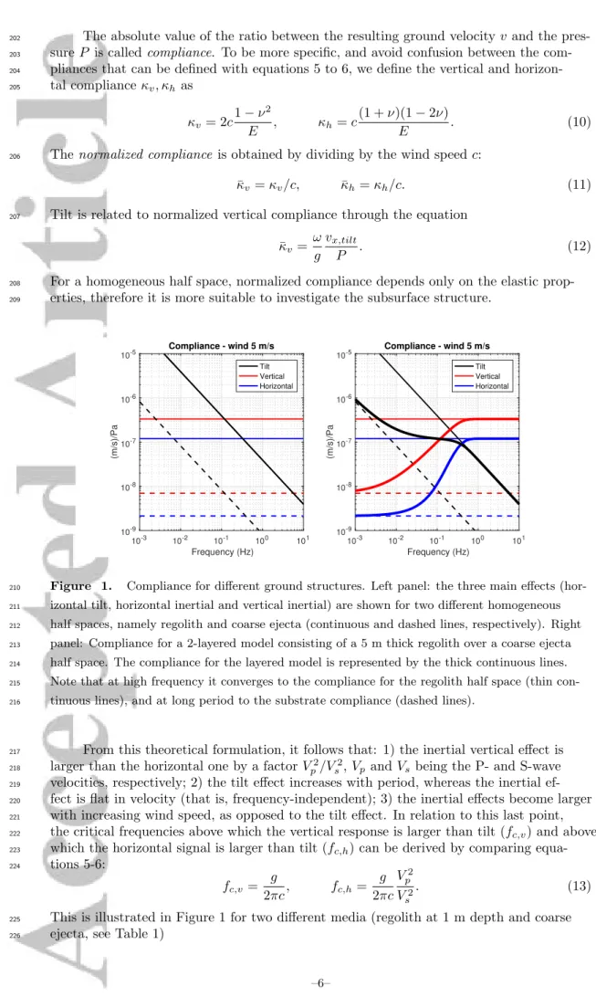
Figure 1. Compliance for different ground structures. Left panel: the three main effects (hor-izontal tilt, hor(hor-izontal inertial and vertical inertial) are shown for two different homogeneous half spaces, namely regolith and coarse ejecta (continuous and dashed lines, respectively). Right panel: Compliance for a 2-layered model consisting of a 5 m thick regolith over a coarse ejecta half space. The compliance for the layered model is represented by the thick continuous lines. Note that at high frequency it converges to the compliance for the regolith half space (thin con-tinuous lines), and at long period to the substrate compliance (dashed lines).
210 211 212 213 214 215 216
From this theoretical formulation, it follows that: 1) the inertial vertical effect is
217
larger than the horizontal one by a factor V2 p/V
2
s, Vp and Vsbeing the P- and S-wave
218
velocities, respectively; 2) the tilt effect increases with period, whereas the inertial
ef-219
fect is flat in velocity (that is, frequency-independent); 3) the inertial effects become larger
220
with increasing wind speed, as opposed to the tilt effect. In relation to this last point,
221
the critical frequencies above which the vertical response is larger than tilt (fc,v) and above
222
which the horizontal signal is larger than tilt (fc,h) can be derived by comparing
equa-223 tions 5-6: 224 fc,v= g 2πc, fc,h= g 2πc Vp2 V2 s . (13)
This is illustrated in Figure 1 for two different media (regolith at 1 m depth and coarse
225
ejecta, see Table 1)
In the case of a horizontally layered half space, no simple formula relating the ground
227
motion to the pressure forcing (the equivalent of equations 5-6 for the homogeneous half
228
space) is available. The solution to the elastostatic equation can however be obtained
229
with a Thomson-Haskell propagator method (Thomson, 1950; Haskell, 1953; Sorrells et
230
al., 1971b). In this case, the compliance becomes frequency dependent: if we assume a
231
single layer lying over a homogeneous half space (Figure 1), it can be seen that at high
232
frequencies the properties of the top layer dominate, whereas at long periods the half space
233
properties become relevant.
234 10-3 10-2 10-1 100 101 Frequency (Hz) 10-9 10-8 10-7 10-6 (m/s)/Pa Vertical compliance 7 8 9 10 log1 0(Pa) 20 10 0 Depth (m) Young modulus 10-3 10-2 10-1 100 101 Frequency (Hz) 10-9 10-8 10-7 10-6 (m/s)/Pa Vertical compliance 7 8 9 10 log1 0(Pa) 20 10 0 Depth (m) Young modulus 10-3 10-2 10-1 100 101 Frequency (Hz) 10-9 10-8 10-7 10-6 (m/s)/Pa Vertical compliance 0 0.2 0.4 20 10 0 Depth (m) Poisson ratio
Figure 2. Sensitivity of vertical ground compliance to various parameters for a 2-layered model. The top row shows the vertical compliance for a wind speed of 5 m/s for the models shown in the bottom row. From left to right, the depth of the second layer, the Young modulus and the Poisson’s ratio in the second layer are varied.
235
236
237
238
We now explore the effect of the various parameters involved in a simple case: we
239
consider a 2-layered model with fixed elastic parameters in the first layer and vary those
240
parameters, and the depth of the discontinuity, in the second layer (Figure 2). We
con-241
clude that: 1) increasing the depth of the second layer shifts the compliance profile
to-242
wards lower frequencies; 2) increasing E of the second layer lowers the compliance
val-243
ues at long and intermediate periods; 3) varying ν does not significantly affect the
re-244
sults.
245
Another way to look at the relationship between subsurface structure, frequency
246
and observed compliance is through sensitivity kernels, as done by e.g. Zha and Webb
247
(2016); Doran and Laske (2019) for seafloor compliance and by Tanimoto and Wang (2019)
248
for surface seismometers. Considering for simplicity E only, its sensitivity kernel S is
de-249
fined by the integral equation
250 δ¯κv ¯ κv = Z 0 −∞ S(z)δE E dz, (14)
where δ indicates a perturbation of the reference model and compliance (Tanimoto &
251
Wang, 2019). An example of the sensitivity kernel for a Mars subsurface model is shown
252
in Figure 3: the results for different frequencies correspond to different penetration depths
253
of the pressure-induced fluctuation, that compare with terrestrial results by Tanimoto
254
and Wang (2019). As pointed out by (Doran & Laske, 2019), however, the sensitivity
kernels are extremely dependent on the reference model, and therefore we did not use
256
them further in our inversion scheme.
257
106 108 1010
Young Modulus (Pa) 20 15 10 5 0 Depth (m) Reference Model -0.4 -0.3 -0.2 -0.1 0 1/m 20 15 10 5 0 Depth (m) Sensitivity Kernels 0.8 Hz 0.3 Hz 0.05 Hz
Figure 3. Depth sensitivity kernels for the Young modulus. The reference model to be per-turbed is shown on the left panel (ν is fixed to 0.25 in all layers). The sensitivity kernels are shown for three different frequencies, and it is clear that at high frequencies the sensitivity to the structure is limited to shallow depth. The computation were done for a wind speed of 5 m/s.
258 259 260 261 10-3 10-2 10-1 100 Frequency (Hz) 10-9 10-8 10-7 10-6 (m/s)/Pa
Compliance - sensitivity to wind speed
Wind speed (m/s) Tilt Vertical Horizontal 2 8 14 20
Figure 4. Sensitivity of ground compliance to wind speed for a two-layered model. The color scale corresponds to the wind speed. The values for wind speed have been chosen as typical for the InSight landing site given the observed wind speeds by APSS.
262
263
264
Another key parameter is the mean wind speed, for which the situation is slightly
265
more complicated. Indeed, increasing the wind speed has two competing effect: first, the
266
inertial effect (both on the vertical and horizontal components) scales like the wind speed,
267
whereas ground tilt does not depend explicitly upon wind. Second, the wavelength of
268
the pressure fluctuation is proportional to the wind speed, thus - for a given frequency
269
- the sensitivity depth (that is, the region determining the compliance observation at the
270
surface) increases with the wind speed. This is shown in Figure 4: for ground tilt, only
271
the sensitivity depth depends on the wind, therefore for a given frequency (and
increas-272
ing stiffness with depth) the compliance decreases when wind increases. For the inertial
273
effect the behavior is more complex, but, generally speaking, stronger winds imply larger
274
pressure noise, although the relationship is frequency dependent and non-linear. These
results show that, apart from the simple case of a homogeneous half space, when
infer-276
ring the subsurface structure from compliance measurements (derived from vertical or
277
tilt seismic signals), it is necessary to take into account the wind speed. Furthermore,
278
analyzing ideal synthetic cases, Kenda et al. (2017) and Murdoch et al. (2017) showed
279
that the tilt effect is sensitive to the pressure field over a larger area. Therefore, when
280
a single pressure sensor is available, estimates derived from the vertical component may
281
be more reliable than tilt-derived estimates. Reconstruction of the trajectory of the
pres-282
sure fluctuations is instead needed when evaluating compliance from ground tilt.
Ad-283
ditionally, since the horizontal components are sensitive both to tilt and ground motion
284
produced by pressure loading, it may be challenging to correctly separate the two effects.
285
For these reasons, in the rest of this work we focused on the compliance observed from
286
the vertical component.
287
2.1 The effect of compaction and confining stress in the regolith layer
288
The theory discussed above can now be applied to the geologic context of the
In-296
Sight landing site to enlighten another key aspect. Pre- and post-landing geological
stud-297
ies (Golombek et al., 2017, 2020; Warner et al., 2019; Ansan et al., 2019) indicate the
298
presence of a layer of sandy regolith, estimated to be between 3 m and 11 m thick based
299
on the analysis of rocky ejecta craters (Warner et al., 2017). Beneath the regolith, stiffer
300
layers of coarse ejecta and fractured bedrock are present. The mechanical properties of
301
the regolith were studied making use of laboratory experiments with Martian simulants
302
(Delage et al., 2017) and theoretical considerations (Morgan et al., 2018). The
result-303
ing pre-landing model has of course large uncertainties (e.g., the actual thickness of the
304
regolith layer, or the density values of the surface layer), however it clearly shows that
305
we cannot assume that the regolith layer has homogeneous elastic properties. Indeed,
306
even neglecting compaction, the elastic properties (for our purposes, the Young
modu-307
lus) strongly depend upon the confining stress, hence upon depth (Morgan et al., 2018).
308
This dependence is illustrated in Figure 5: the reference model by Morgan et al. (2018)
309
is shown for different thicknesses of the regolith and compared to the corresponding
ho-310
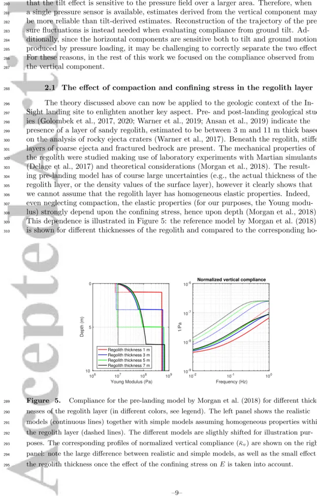
106 107 108 109 Young Modulus (Pa) 10 5 0 Depth (m) Regolith thickness 1 m Regolith thickness 3 m Regolith thickness 5 m Regolith thickness 7 m 10-2 10-1 100 Frequency (Hz) 10-9 10-8 10-7 10-6 1/Pa
Normalized vertical compliance
Figure 5. Compliance for the pre-landing model by Morgan et al. (2018) for different thick-nesses of the regolith layer (in different colors, see legend). The left panel shows the realistic models (continuous lines) together with simple models assuming homogeneous properties within the regolith layer (dashed lines). The different models are sligthly shifted for illustration pur-poses. The corresponding profiles of normalized vertical compliance (¯κv) are shown on the right
panel: note the large difference between realistic and simple models, as well as the small effect of the regolith thickness once the effect of the confining stress on E is taken into account.
289 290 291 292 293 294 295
mogeneous models. It can be seen that E increases by a factor 4 over the first meter,
311
and by an order of magnitude at 5 m depth.
312
For this set of models we computed the normalized compliance as described above
313
(by densely discretizing the vertical profile of E every 5 cm in order to mimic the effect
314
of a continuous increase). The compliance profiles exhibit a large difference between
sim-315
ple models (that is, with a homogeneous regolith layer) and models accounting for the
316
effects of confining stress (Figure 5). Furthermore, once the confining stress is
consid-317
ered, the effect of different regolith thickness is mitigated, and therefore it becomes
dif-318
ficult to infer this parameter. This point is extremely important for the inversion
strat-319
egy and for the interpretation of inversion results.
320
3 Compliance observations at the InSight landing site
321
3.1 Dataset for this study
322
InSight landed on November 26, 2018 at Elysium Planitia and the SEIS experiment
323
was deployed on the ground on Sol 22 and covered with the Wind and Thermal Shield
324
on Sol 66 (Lognonn´e et al., 2020; Banerdt et al., 2020). Since Sol 73, the SEIS
seismome-325
ters have been functioning in the nominal mode of operation producing an almost
con-326
tinuous high-quality dataset (Lognonn´e et al., 2020). SEIS includes two three-axis
seis-327
mometers, the VBBs (Very Broad Band) and SPs (Short Period) fully described in Lognonn´e
328
et al. (2019). In this study, we focused on the VBB data since these sensors have
bet-329
ter performances in the frequency range of our interest, that is below 1 Hz. The VBBs
330
produce two different datastreams: the VEL and POS outputs (proportional to ground
331
velocity and acceleration, respectively). The pre-processing of seismic data includes
stan-332
dard procedures (removal of the transfer function to retrieve ground motion in
physi-333
cal units, axis recombination to the standard geographical frame Vertical/North/East).
334
The geographic north with respect to the SEIS reference frame was determined through
335
a sundial (Savoie et al., 2019). The APSS experiment did not require a deployment and
336
monitored the atmospheric and magnetic environment almost continuously since the
be-337
ginning of operations. The meteorological channels used in this work are limited to
cal-338
ibrated pressure and wind data (Banfield et al., 2020). We analyzed data from Sol 73
339
to Sol 227, all of which are publicly available (InSight Mars SEIS data Service, 2020).
340
To ensure that the comparison of seismic and pressure data gives access to the ground
346
compliance as described in Section 2, it is necessary to check whether the seismic
sig-347
nals are actually generated by the pressure fluctuations (Murdoch et al., 2017). An
ef-348
ficient way to do it is to measure the coherence between the time series and hence
mea-349
sure the amount of the power spectral density of the seismic signal that is explained by
350
pressure variations. This is shown in Figure 6 for Sol 114 through a cohero-gram,
illus-351
trating how coherence varies with local time for the three seismic axis. It can be seen
352
that the background coherence level is low during the nighttime and it increases during
353
the daytime when convective turbulence in the Planetary Boundary Layer is strong (Spiga
354
et al., 2018; Banfield et al., 2020). However, zooming in in the daytime shows that high
355
coherence is mostly limited to the occurrence of strong pressure signals, mainly pressure
356
drops that indicate encounters with convective vortices (dust devils, if enough dust
par-357
ticles are carried within the vortex). The cohero-grams of Figure 6 show that the high
358
coherence (say, above 0.8) between pressure and seismic time series required for
compli-359
ance analysis is generally limited to the band 0.02-0.9 Hz. We will thus focus on this
lim-360
ited range, although episodes with high coherence at higher (or lower) frequency are
pos-361
sible and can be individually studied. For a more complete analysis of the coherence and
362
the observed effects of pressure fluctuations, we refer to the companion paper by Garcia
363
et al. (2020).
0 5 10 15 20 −2 −10 Pa
Pressure
12.6 12.8 13.0 13.2 13.4 −2 −10 PaPressure
0 5 10 15 20 10−2 10−1 100 HzVertical/Pressure coherence
12.6 12.8 13.0 13.2 13.4 10−2 10−1 100 HzVertical/Pressure coherence
0 5 10 15 20 10−2 10−1 100 HzEast/Pressure coherence
12.6 12.8 13.0 13.2 13.4 10−2 10−1 100 HzEast/Pressure coherence
0 5 10 15 20Local Mean Solar Time 10−2 10−1 100 Hz
North/Pressure coherence
12.6 12.8 13.0 13.2 13.4Local Mean Solar Time 10−2 10−1 100 Hz
North/Pressure coherence
0.2 0.4 0.6 0.8Figure 6. Coherence between the pressure and very-broad band (VBB) seismic signals over Sol 114. The pressure time series are high-pass filtered at 600 s. Coherence ranges from 0 (blue) to 1 (yellow). It appears that the coherence is high mostly for short time windows corresponding to strong pressure signals, e.g. convective vortices during the daytime. The right panels are a zoom into 12.5-13.5 Local time.
341
342
343
344
345
3.2 Measurements from dust-devil convective vortices
365
Since they often exhibit a large coherence between pressure and seismic signals,
con-369
vective vortices are well suited to perform compliance measurements (Kenda et al., 2017).
370
We considered about 360 vortices encountered between Sol 73 and Sol 169. From the whole
371
catalog of pressure drops larger than 0.25 Pa, we selected (in an almost-automated
pro-372
cedure, including a final manual quality check) a subset of events i) that had a large
co-373
herence; ii) whose vertical seismic signal could be simply modeled with a single
propor-374
tionality coefficient based on the theory of Section 2. In particular, we considered
vor-375
tex encounters for which the coherence between seismic and pressure time series have
376
a coherence larger than 0.5. The procedure, described in more details in Garcia et al.
377
(2020) and Lognonn´e et al. (2020), gives - for each event - a measurement of the
appar-378
ent compliance in a certain frequency range (determined by requiring a reduction both
379
of the coherence with pressure and of the spectral density of the seismic signal). By
tak-380
ing as ambient wind speed the average value over 1 minute before and after the vortex
381
encounter (removing the vortex encounter itself), we derive the normalized compliance
382
(Figure 7).
383
Based on the discussion in Section 2, and in particular on the effect of the
ambi-384
ent wind on the apparent normalized compliance for layered media, one could claim that
385
it is not possible to derive statistics from events occurring in different wind conditions.
386
However, clustering of the resulting compliance measurements based on the wind speed,
387
does not show significantly different results (Figure 7). This means that the variance of
388
the compliance values alone, taken here as a measure of the uncertainty, dominates over
389
the effect of wind speed when enough events are considered. Therefore, we decided to
390
consider the whole compliance distribution regardless of wind speed (and to use the
10
−210
−110
0Frequency (Hz)
10
−910
−810
−7 κv(1/Pa)
# Events
wind<4.5m/s
10
−210
−110
0Frequency (Hz)
10
−910
−810
−7 κv(1/Pa)
# Events
4.5m/s<wind<6m/s
10
−210
−110
0Frequency (Hz)
10
−910
−810
−7 κv(1/Pa)
# Events
wind>6m/s
10
−210
−110
0Frequency (Hz)
10
−910
−810
−7 κv(1/Pa)
# Events
all wind
0
5
10
15
20
0
10
20
30
40
0
5
10
15
20
25
30
35
0
20
40
60
80
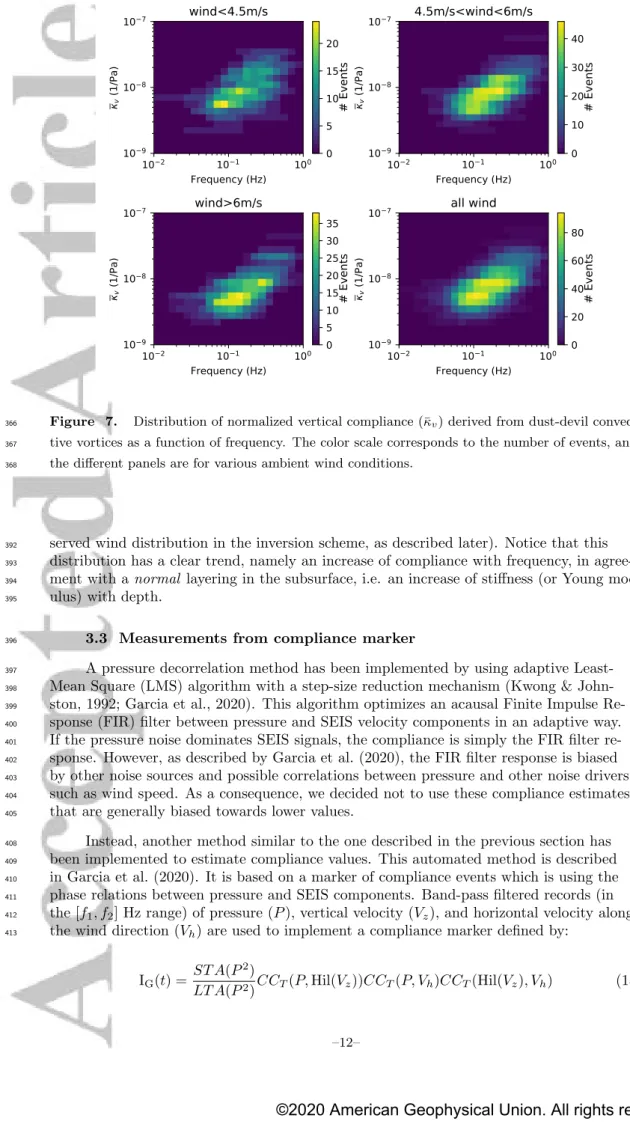
Figure 7. Distribution of normalized vertical compliance (¯κv) derived from dust-devil
convec-tive vortices as a function of frequency. The color scale corresponds to the number of events, and the different panels are for various ambient wind conditions.
366
367
368
served wind distribution in the inversion scheme, as described later). Notice that this
392
distribution has a clear trend, namely an increase of compliance with frequency, in
agree-393
ment with a normal layering in the subsurface, i.e. an increase of stiffness (or Young
mod-394
ulus) with depth.
395
3.3 Measurements from compliance marker
396
A pressure decorrelation method has been implemented by using adaptive
Least-397
Mean Square (LMS) algorithm with a step-size reduction mechanism (Kwong &
John-398
ston, 1992; Garcia et al., 2020). This algorithm optimizes an acausal Finite Impulse
Re-399
sponse (FIR) filter between pressure and SEIS velocity components in an adaptive way.
400
If the pressure noise dominates SEIS signals, the compliance is simply the FIR filter
re-401
sponse. However, as described by Garcia et al. (2020), the FIR filter response is biased
402
by other noise sources and possible correlations between pressure and other noise drivers
403
such as wind speed. As a consequence, we decided not to use these compliance estimates
404
that are generally biased towards lower values.
405
Instead, another method similar to the one described in the previous section has
408
been implemented to estimate compliance values. This automated method is described
409
in Garcia et al. (2020). It is based on a marker of compliance events which is using the
410
phase relations between pressure and SEIS components. Band-pass filtered records (in
411
the [f1, f2] Hz range) of pressure (P ), vertical velocity (Vz), and horizontal velocity along
412
the wind direction (Vh) are used to implement a compliance marker defined by:
413
IG(t) =
ST A(P2)
10−8 Compliance (1/Pa) 10−1 Frequency (Hz) 0 5 10 15 20 25 30 35 Weight 10 2 10 1 100 Frequency (Hz) No rmaliz ed compliance (1/P a) 10 9 10 8 10 7 10−8 Compliance (1/Pa) 10−1 Frequency (Hz) 0 5 10 15 20 25 30 35 Weight 0 10 20 30 Weight 1
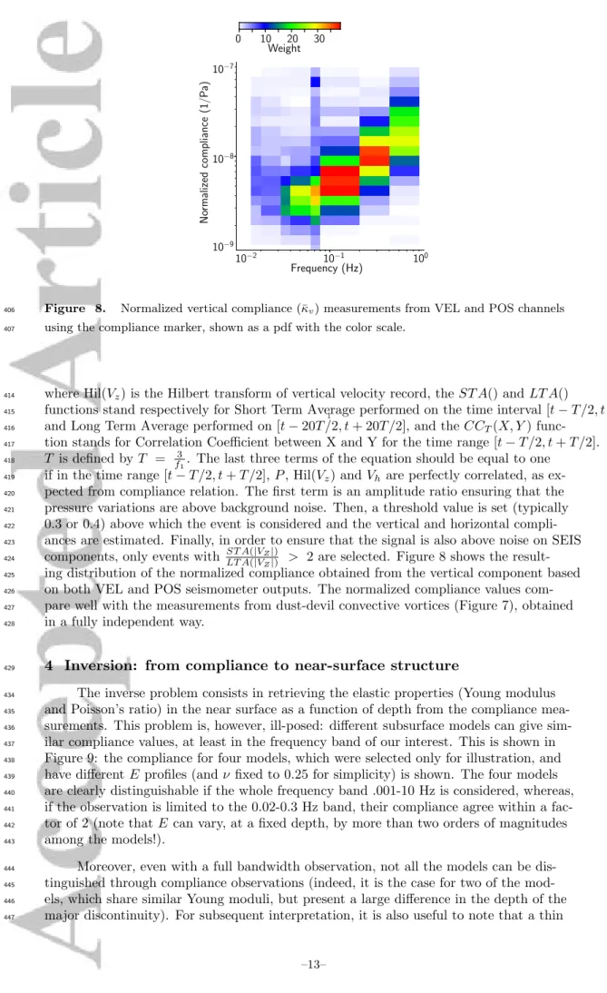
Figure 8. Normalized vertical compliance (¯κv) measurements from VEL and POS channels
using the compliance marker, shown as a pdf with the color scale.
406
407
where Hil(Vz) is the Hilbert transform of vertical velocity record, the ST A() and LT A()
414
functions stand respectively for Short Term Average performed on the time interval [t− T/2, t + T/2],
415
and Long Term Average performed on [t− 20T/2, t + 20T/2], and the CCT(X, Y )
func-416
tion stands for Correlation Coefficient between X and Y for the time range [t− T/2, t + T/2].
417
T is defined by T = 3
f1. The last three terms of the equation should be equal to one 418
if in the time range [t− T/2, t + T/2], P , Hil(Vz) and Vh are perfectly correlated, as
ex-419
pected from compliance relation. The first term is an amplitude ratio ensuring that the
420
pressure variations are above background noise. Then, a threshold value is set (typically
421
0.3 or 0.4) above which the event is considered and the vertical and horizontal
compli-422
ances are estimated. Finally, in order to ensure that the signal is also above noise on SEIS
423
components, only events with ST A(|VZ|)
LT A(|VZ|) > 2 are selected. Figure 8 shows the result-424
ing distribution of the normalized compliance obtained from the vertical component based
425
on both VEL and POS seismometer outputs. The normalized compliance values
com-426
pare well with the measurements from dust-devil convective vortices (Figure 7), obtained
427
in a fully independent way.
428
4 Inversion: from compliance to near-surface structure
429
The inverse problem consists in retrieving the elastic properties (Young modulus
434
and Poisson’s ratio) in the near surface as a function of depth from the compliance
mea-435
surements. This problem is, however, ill-posed: different subsurface models can give
sim-436
ilar compliance values, at least in the frequency band of our interest. This is shown in
437
Figure 9: the compliance for four models, which were selected only for illustration, and
438
have different E profiles (and ν fixed to 0.25 for simplicity) is shown. The four models
439
are clearly distinguishable if the whole frequency band .001-10 Hz is considered, whereas,
440
if the observation is limited to the 0.02-0.3 Hz band, their compliance agree within a
fac-441
tor of 2 (note that E can vary, at a fixed depth, by more than two orders of magnitudes
442
among the models!).
443
Moreover, even with a full bandwidth observation, not all the models can be
dis-444
tinguished through compliance observations (indeed, it is the case for two of the
mod-445
els, which share similar Young moduli, but present a large difference in the depth of the
446
major discontinuity). For subsequent interpretation, it is also useful to note that a thin
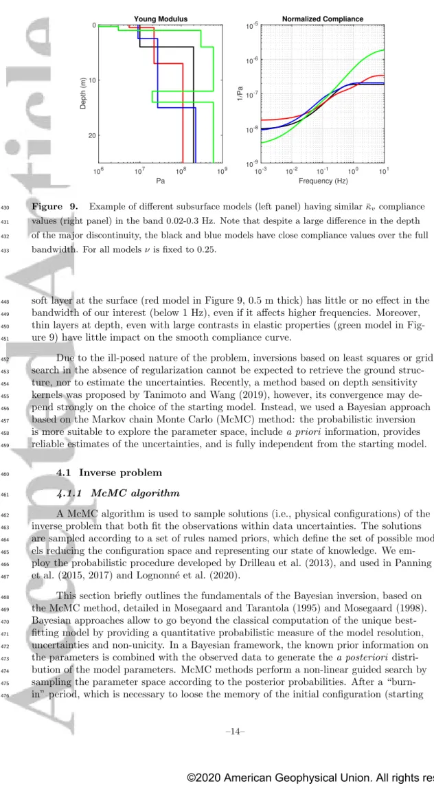
10-3 10-2 10-1 100 101 Frequency (Hz) 10-9 10-8 10-7 10-6 10-5 1/Pa Normalized Compliance 106 107 108 109 Pa 20 10 0 Depth (m) Young Modulus
Figure 9. Example of different subsurface models (left panel) having similar ¯κvcompliance
values (right panel) in the band 0.02-0.3 Hz. Note that despite a large difference in the depth of the major discontinuity, the black and blue models have close compliance values over the full bandwidth. For all models ν is fixed to 0.25.
430
431
432
433
soft layer at the surface (red model in Figure 9, 0.5 m thick) has little or no effect in the
448
bandwidth of our interest (below 1 Hz), even if it affects higher frequencies. Moreover,
449
thin layers at depth, even with large contrasts in elastic properties (green model in
Fig-450
ure 9) have little impact on the smooth compliance curve.
451
Due to the ill-posed nature of the problem, inversions based on least squares or grid
452
search in the absence of regularization cannot be expected to retrieve the ground
struc-453
ture, nor to estimate the uncertainties. Recently, a method based on depth sensitivity
454
kernels was proposed by Tanimoto and Wang (2019), however, its convergence may
de-455
pend strongly on the choice of the starting model. Instead, we used a Bayesian approach
456
based on the Markov chain Monte Carlo (McMC) method: the probabilistic inversion
457
is more suitable to explore the parameter space, include a priori information, provides
458
reliable estimates of the uncertainties, and is fully independent from the starting model.
459
4.1 Inverse problem
460
4.1.1 McMC algorithm
461
A McMC algorithm is used to sample solutions (i.e., physical configurations) of the
462
inverse problem that both fit the observations within data uncertainties. The solutions
463
are sampled according to a set of rules named priors, which define the set of possible
mod-464
els reducing the configuration space and representing our state of knowledge. We
em-465
ploy the probabilistic procedure developed by Drilleau et al. (2013), and used in Panning
466
et al. (2015, 2017) and Lognonn´e et al. (2020).
467
This section briefly outlines the fundamentals of the Bayesian inversion, based on
468
the McMC method, detailed in Mosegaard and Tarantola (1995) and Mosegaard (1998).
469
Bayesian approaches allow to go beyond the classical computation of the unique
best-470
fitting model by providing a quantitative probabilistic measure of the model resolution,
471
uncertainties and non-unicity. In a Bayesian framework, the known prior information on
472
the parameters is combined with the observed data to generate the a posteriori
distri-473
bution of the model parameters. McMC methods perform a non-linear guided search by
474
sampling the parameter space according to the posterior probabilities. After a
“burn-475
in” period, which is necessary to loose the memory of the initial configuration (starting
model), McMC methods perform a non-linear guided search by sampling the
parame-477
ter space according to the posterior probabilities.
478
Let us denote by p the parameters of our model and d the data, respectively. The
479
data are related to the parameters through the equation, d = A(p), where the non-analytic
480
and non-linear operator A represents the forward problem discussed in Section 2.
Ex-481
plicitly, the parameters are the depths, the Young modulus and Poisson’s ratio of each
482
layer. In the Bayesian framework, a set of parameters is randomly chosen at each
iter-483
ation. The corresponding E and ν profiles are then used to compute the compliance as
484
a function of frequency. The solutions of the inverse problem are described by the
pos-485
terior probabilities P (p|d) that the parameters are in a configuration p given the data
486
are in a configuration d. The parameter space is sampled according to P (p|d). Bayes’
487
theorem links the prior distribution P (p) and the posterior distribution P (p|d),
488
P(p|d) = XP(d|p)P (p) p∈M
P(d|p)P (p), (16)
whereM denotes all the configurations in the parameter space. P (p) defines the prior
489
distribution, i. e. the set of possible models which reduce the configuration space and
490
represents our state of knowledge.
491
The probability distribution P (d|p) is a function of the misfit S(d, A(p)), which
492
determines the difference between the observed data d and the computed synthetic data
493
A(p). The input compliances as a function of frequency data are provided in the form
494
of 2D matrices (Figures 7 and 8), which give a weight to each (frequency, compliance)
495
couple. In practice, each time a new model is randomly sampled, a weight is given for
496
each frequency according to compliance value in the 2D matrix. The sum of the weights
497
for all the frequencies gives the misfit value. To estimate the posterior distribution (Eq.
498
16), we employ the Metropolis algorithm (Metropolis et al., 1953; Hastings, 1970), which
499
samples the model space with a sampling density proportional to the unknown
poste-500
rior probability density function. This algorithm relies on a randomized decision rule which
501
accepts or rejects the proposed model according to its fit to the data and the prior.
502
4.1.2 Model parameterization and a priori conditions
503
The Bayesian formulation enables a priori knowledge to be accounted for. We choose
504
to compare two different parameterizations, one with relatively few a priori conditions
505
on the Young modulus and Poisson’s ratio (called M1), and another one using physical
506
assumptions (called M2). Table 2 summarises the inverted parameters and the prior bounds
507
considered for M1 and M2 models. It is worth noting that these parametrizations cover
508
a range that is larger than the realistic properties of the expected rocks, however this
509
does not affect the inversion results and guarantees instead the robustness of the
inver-510
sion scheme. Indeed, considering a large parameter space for the inverse problem ensures
511
that no physically acceptable region may be missed because of boundary effects.
512
The first set of models is parameterized using several layers of variable thicknesses
513
(a good compromise turned out to be 8 layers, apart for a synthetic test where we used
514
2 layers only). The varying parameters are the depth of each layer, E and ν for each
con-515
sidered layer. The parameters are randomly sampled in relatively wide parameter spaces
516
(Table 2), with no assumption on the depth of the structural discontinuities.
517
A second set of models is parameterized considering physical assumptions in the
520
regolith. The model is divided into two parts: the regolith and an underlying
geologi-521
cal unit (expected, but not requested, to be stiffer). This unit could be made of coarse
522
ejecta, fractured bedrock, or basaltic lava flows, or a combination of those, but due to
523
limited resolution we do not attempt to extract information about further layering. In
524
the regolith, we consider that the medium is densely compacted, using the empirical law
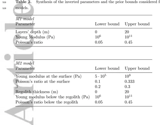
Table 2. Synthesis of the inverted parameters and the prior bounds considered for M1 and M2 models.
518
519
M1 model
Parameter Lower bound Upper bound
Layers’ depth (m) 0 20
Young Modulus (Pa) 106 1011
Poisson’s ratio 0.05 0.45
M2 model
Parameter Lower bound Upper bound
Young modulus at the surface (Pa) 5· 105 108
Poisson’s ratio at the surface 0.1 0.333
β 0.2 0.3
Regolith thickness (m) 0 20
Young modulus below the regolith (Pa) 106 1011
Poisson’s ratio below the regolith 0.05 0.45
from Morgan et al. (2018). E and ν at the surface are randomly sampled during the
in-526
version scheme, within the ranges detailed in Table 2. Equations 1 and 20 from Morgan
527
et al. (2018) are then used to compute the whole E and ν profile as a function of depth
528
within the regolith layer. The uncertainty on this compaction model is taken into
ac-529
count by varying the experimentally determined and non-dimensional exponent β of
equa-530
tion 20 from Morgan et al. (2018). This β parameter describes the exponential increase
531
of the elastic parameters with confining stress. The thickness of the regolith layer is
ran-532
domly sampled between 0 m and 20 m. Below the regolith, a single homogeneous unit
533
is assumed, whose Young modulus and Poisson’s ratio can vary within the same range
534
of values as for the M1 models.
535
Figures 10a and 10b show the prior distributions of E profiles of M1 and M2
mod-545
els, respectively, assuming the conditions detailed in Table 2. Both the a priori
assump-546
tions and the sampling of the models lead to non uniform distributions. Concerning M1
547
models (Figure 10a), the pdf does not vary significantly with depth, but the center of
548
the parameter space is better sampled than the bounds. In the McMC algorithms, new
549
models are proposed by randomly perturbing the previously accepted model. Here, the
550
sampling of the parameter space is performed using a continuous proposal function.
Defin-551
ing the t-th and the (t+1)-th value of a parameter p, as pt i and p
t+1
i , respectively, then
552
the subsequent step may be defined as pt+1i = p t
i + wi, where wi is the t-th stepsize,
553
randomly sampled from a normal distribution with zero mean. A Gaussian probability
554
density distribution, centred at pt
i is classically used to randomly sample the p t+1
i , which
555
explains why for a given depth, the pdf decreases when moving away from the center of
556
the parameter space. Contrary to the M1 pdf (Figure 10a), the a priori distribution of
557
M2 models (Figure 10b) is strongly depth-dependent, because compaction and
confin-558
ing stress are accounted for in the regolith (Morgan et al., 2018). The pdf is spread as
559
a function of depth, because of the homogeneous layer below the regolith. As for the M1
560
pdf, the bounds of the distribution are less sampled. Note that we verified the efficiency
561
of the inversion process and the sampling by realizing several synthetic tests with extreme
562
values of the parameters space as input. The tested models were retrieved with success
563
by the algorithm. We stress that no covariance structure is imposed to the prior. This
564
choice was made to avoid including prior information in this first study and to explore
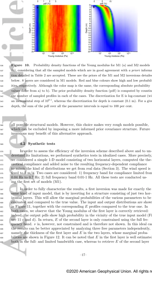
0 1 2 3 4 5 6 7 8 9 10 11 12 13 14 15 16 17 18 19 20 Depth (m) 107 108 109 1010
Young modulus (Pa)
0 1 2 3 pdf (%) 0 1 2 3 4 5 6 7 8 9 10 11 12 13 14 15 16 17 18 19 20 Depth (m) 107 108 109 1010
Young modulus (Pa)
0 5 10
pdf (%)
a b
Figure 10. Probability density functions of the Young modulus for M1 (a) and M2 models (b), considering that all the sampled models which are in good agreement with a priori informa-tion detailed in Table 2 are accepted. These are the priors of the M1 and M2 inversions detailed below. 8 layers are considered in M1 models. Red and blue colours show high and low probabil-ities, respectively. Although the color map is the same, the corresponding absolute probability values differ from a) to b). The prior probability density function (pdf) is computed by counting the number of sampled profiles in each of the cases. The discretization for E is log-constant (with an incremental step of 100.1, whereas the discretization for depth is constant (0.1 m). For a given depth, the sum of the pdf over all the parameter intervals is equal to 100 per cent.
536 537 538 539 540 541 542 543 544
all possible structural models. However, this choice makes very rough models possible,
566
which can be excluded by imposing a more informed prior covariance structure. Future
567
inversions may benefit of this alternative approach.
568
4.2 Synthetic tests
569
In order to assess the efficiency of the inversion scheme described above and to
un-570
derstand its limitations, we performed synthetics tests in idealized cases. More precisely,
571
we considered a simple 1-D model consisting of two horizontal layers, computed the
the-572
oretical compliance and added noise to the resulting frequency-dependent compliance
573
to mimic the kind of distributions we get from real data (Section 3). The wind speed is
574
fixed to 5 m/s. Two cases are considered: 1) frequency band for compliance limited from
575
0.04 Hz to 0.7 Hz; 2) full frequency band 0.01-1 Hz. All these tests are conducted
us-576
ing the first set of models (M1).
577
In order to fully characterize the results, a first inversion was made for exactly the
597
same kind of input model, that is by inverting for a structure consisting of just two
hor-598
izontal layers. This will allow the marginal probabilities of the various parameters to be
599
evaluated and compared to the true value. The input and output distributions are shown
600
in Figure 11, together with the corresponding E profiles compared to the true one. In
601
both cases, we observe that the Young modulus of the first layer is correctly retrieved:
602
indeed, the output pdfs show high probability in the vicinity of the true input model
(Fig-603
ure 11 c and d). In return, E of the second layer is only constrained using the full
fre-604
quency band. ν is, however, not constrained and is therefore not shown. In this ideal case,
605
the results can be better appreciated by analyzing three free parameters independently,
606
namely the thickness of the first layer and E in the two layers, whose marginal
proba-607
bilities are shown in Figure 12. It can be noted that E in the first layer is well estimated
608
both in the full- and limited bandwidth case, whereas to retrieve E of the second layer
knowledge of the full bandwidth compliance is necessary. The thickness of the first layer
610
is, however, not as well constrained as the Young modulus. Nevertheless, analysis of the
611
fit suggest that the right thickness can be inferred by minimizing the fit, as suggested
612
by the best-fit models shown in Figure 11 e and f, which cluster around the true
thick-613
ness of 4 m. A more careful analysis of the fit as a function of thickness (Figure 13)
con-614
firms this interpretation. In the limited bandwidth case, however, the fit for thicknesses
615
of about 4 m is, in a statistical sense, not better as compared to the one for other
val-616
ues. For the full bandwidth case, instead, the fit distribution is significantly better for
617
thickness values close to the true one.
618
An additional inversion test on the same dataset was made by relaxing the
assump-621
tion on the number of layers, increasing it to 8 at random depths (recall that the input
622
model had only two layers). The inversion results are shown in Figure 14. As expected,
623
the resolution at intermediate depth is in this case worse (since thin layers with arbitrary
624
Young moduli can be inserted without significantly affecting the compliance profile), but
625
E in the first layer is correctly retrieved, and interestingly its thickness as well. Indeed,
626
although it is not immediately clear how to define a discontinuity from pdfs, it appears
627
that resolution is good down to about 4 m, which is the true thickness of the first layer.
628
Moreover, in the full-bandwidth case (Figure 14 b and d), E towards 20 m (and below)
629
is correctly retrieved. Note that having better resolution below a certain depth is related
630
to the inversion scheme, since fixing a half-space structure for the lowermost layer
trig-631
gers the convergence of the models towards the true value of E. At intermediate depths,
632
instead, small layers with almost arbitrary values of E can be inserted, producing a less
633
constrained distribution.
634
4.3 Inversion of Mars data
635
4.3.1 Inversion assuming a layered structure
636
The first inversion performed on ground compliance observed by InSight (Section
637
3) was done without assuming a priori knowledge of the Martian near surface from
ge-638
ology and geotechnical experiments. Hence, we considered the M1 model class (Table
639
2) and assumed a horizontally layered structure (8 layers) over a homogeneous half space.
640
In all inversions of Martian data, the wind speed was chosen in the distribution observed
641
for the corresponding dataset.
642
The results are presented in Figure 15. First of all it should be noticed that the
649
inversion scheme is able to reproduce the observed distributions of compliance with
fre-650
quency (Figure 15 a and b). Moreover, as both measurement techniques exhibit a trend
651
of compliance with frequency, the retrieved vertical profiles of E are characterized by an
652
increase of stiffness with depth (Figure 15 c and d), suggesting the presence of a major
653
discontinuity between 3 and 15 m depth (see Section 5 for an interpretation of these
re-654
sults). In addition to this, the distribution is relatively well constrained close to the
sur-655
face and below 15 m depth, whereas at intermediate depths the acceptable values for E
656
are spread. This was also the case for the synthetic test described above (Figure 14 d)
657
and inherently depends on the possibility of adding thin layers with arbitrary elastic
pa-658
rameters at intermediate depths without affecting the compliance profile (Figure 9).
In-659
deed, where a half space structure is imposed, the models have no more the freedom to
660
include layers with little effect on the observed compliance and, accordingly, cluster
to-661
wards Young modulus values that fit the data.
662
4.3.2 Inversion assuming a compaction profile
663
A second inversion assumed a compaction profile in the regolith as well as the
ef-664
fect of confining stress on E as described in Section 4.1.2 (M2 model class). In this case
665
the general behavior of the retrieved Young modulus (Figure 16 c and d) is similar for
the inversion based on dust-devil vortex events and compliance marker. Note however
667
that the increase of the Young modulus in the regolith layer (corresponding to the
con-668
tinuously bend region close to the surface) is strongly determined from the prior
assump-669
tions (Figure 10 b). Nevertheless, a comparison with the prior distribution suggests a
670
relatively thin regolith layer, and a Young modulus below the regolith layer constrained
671
by the inversion procedure. It is also worth noting that E below the regolith layer is
sim-672
ilar to those found in the inversion without a priori. These points, together with the
gen-673
eral interpretation of the results, will be further discussed in Section 5.
674
5 Discussion
678
In order to avoid over- or misinterpretations of the inversion results presented in
679
Section 4.3, we critically review here those results and their implications in terms of the
680
near-surface structure at the InSight landing site. To do it, we analyze some key
param-681
eters summarizing the outputs of the inversions (the Young modulus at the very surface
682
and at depth, and the regolith thickness) and compare them with pre-landing
expecta-683
tions.
684
First of all, we consider the Young modulus at the very surface as retrieved from
685
the two proposed inversion schemes (Figure 17 a and c). The pre-launch proposed Young
686
modulus at the surface is 7.5 MPa (Morgan et al., 2018, Table 1), increased to about 20
687
MPa beneath the SEIS feet due to the weight of the sensor assembly. The inversions
con-688
sidering a layered structure give the 1σ confidence intervals of 30-200 MPa for the
dust-689
devil vortices dataset, and 30-125 MPa for the compliance marker inversion (Table 3).
690
Assuming a density of 1300 kg/m3and ν=0.25, we express these ranges by using the
ex-691
pression of the P-wave velocity: Vp =
(1−ν)E
ρ(1+ν)(1−2ν). This provides ranges of 166-430 and
692
166-340 m/s, respectively. These values are significantly higher than both the pre-launch
693
one and those measured by the HP3travel times, suggesting about 120 m/s (Lognonn´e
694
et al., 2020). The lower bounds are comparable to those proposed by Lognonn´e et al.
695
(2020) for similar compliance inversions. In both cases, however, it should be kept in mind
696
that because of the limited bandwidth of the observations (especially towards high
fre-697
quencies), the measurements are not sensitive to very shallow layers. Moreover, it can
698
be noticed that the a posteriori distribution is asymmetric (Figure 17 a), with low
val-699
ues of E more likely than very high values.
700
When taking into account the effect of confining stress (M2 inversion, Figure 17
707
c), the 1σ interval for E at the surface is lowered to 12-31 MPa (dust-devil convective
708
vortices) and 12-25 MPa (compliance marker), values which are much closer to the
pre-709
landing estimates. These provide P-wave velocities in the range 136-152 m/s for the two
710
median values, slightly higher than the measure based on HP3-hammering travel times
711
(Vp=120 m/s). However, the difference between the M1 and M2 inversions suggests that
712
the inversion scheme has a major impact on the retrieved Young modulus at the surface.
713
We thus recommend to consider these values with the due attention to the inversion
pro-714
cedure.
715
The Young modulus at 20 m depth (Figure 17 b and d) has less prominent
prob-719
ability peaks, but the distribution is still significantly different from the prior.
Interest-720
ingly, in this case all the inversions produce consistent and similar results (Table 3) with
721
a median value of 0.6-1 GPa fully compatible with a layer of coarse ejecta. This strongly
722
suggests that the observed compliance is sensitive to a relatively stiff layer of rock at some
723
depth and to an integrated value in the regolith layer. However, note that the confidence
724
intervals for E at depth span one order of magnitude, apart for the M2 inversion of the
725
compliance-marker measurements, for which the a posteriori uncertainty is roughly a
fac-726
tor of 2. In addition, the precise depth is not straightforward to infer: in particular the
727
depth of 20 m is the one where we put the homogeneous half space in the M1 inversions,