Robust and adaptable dynamic response reshaping of flexible structures

an author's

https://oatao.univ-toulouse.fr/25482

https://doi.org/10.1016/j.jsv.2019.115086

Preda, Valentin and Sanfedino, Francesco and Bennani, Samir and Boquet, Fabrice and Alazard, Daniel Robust and

adaptable dynamic response reshaping of flexible structures. (2020) Journal of Sound and Vibration, 468. 1-22. ISSN

0022460X

Robust and adaptable dynamic response reshaping of flexible

structures

Valentin Preda

a,∗

_{, Francesco Sanfedino}

b

_{, Samir Bennani}

a

_{, Fabrice Boquet}

a

_,

Daniel Alazard

b

a_{European Space Agency (GNC, AOCS & Pointing Division), ESTEC, Noordwijk, the Netherlands} b_{Institut Supérieur de l’Aéronautique et de l’Espace (ISAE-SUPAERO), Toulouse, France}

Keywords: Flexible structures Identification Physical modeling Robust control Worst-case analysis a b s t r a c t

This paper outlines a complete methodology for designing a control system that reshapes the dynamic response of the flexible structure to robustly match the dynamics of a given adapt-able reference model. The procedure was experimentally verified on a setup developed at the European Space Agency, consisting of a cantilevered flexible plate actuated by two shakers. Angular displacements at the free tip of the plate were measured with sub-microradian res-olution using a laser autocollimator. Following a comprehensive system identification phase, mathematical models of the uncertain plant were extracted. The models reliably fit the exper-imental data and were used to synthesize a low order and high bandwidth structured Linear Parameter Varying controller. The controller was designed by taking into account the limits of achievable performance and the closed loop effectively constrained the flexible structure to behave like it was made out of an adaptable material. The robust stability and worst case performances were assessed by means of a structured singular value analysis and excellent agreement between theoretical predictions and experimental results was observed.

1. Introduction

1.1. Background and motivation

The fairing size envelopes of current launchers impose substantial constraints on spacecraft design. To overcome these size restrictions, a significant number of modern telecommunication, Earth observation, and science missions rely on large

deploy-able structures to meet their performance goals [1,2]. There is currently a strong interest in developing ultralight, compactly

packable [3,4] structures that can be deployed [5] or even manufactured [6] and assembled in space. However, as structures

become larger and more flexible they become more susceptible to mechanical vibrations due to the low structural damping in the materials and the absence of other forms of damping in the vacuum of space. Moreover, both ESA and other space agencies are preparing missions that require extremely high pointing accuracy and an ultra-quiet environment for the vibration-sensitive

instruments [7,8]. This is a very challenging problem since a multitude of critical on-board equipment such as reaction wheels,

cryocoolers, solar array drives and antenna pointing mechanisms generate significant levels of mechanical vibrations during

operation [9]. These vibrations can easily propagate and interact with the large number of lightly damped and closely spaced

flexible modes of the spacecraft structure [10]. With the advent of increasingly powerful imaging sensors and more lightweight

∗

Corresponding author.

E-mail address:valentin.preda@esa.int(V. ).

materials, understanding and controlling the propagation of these microvibrations and their dynamic interaction is one of the

most critically important problem areas in spacecraft systems engineering [7].

Over the years, a wide variety [9] of microvibration isolation systems have been developed or proposed in an effort to tackle

this problem. Most of them focus on mechanical isolation of the noisy equipment and/or of the sensitive payload from the rest

of the spacecraft structure [11–17]. For some observation missions, active and adaptive optics [18–20] are a promising

technol-ogy to perform wavefront correction and improve pointing stability at the payload level. Another complementary strategy is to actively control the spacecraft structure itself and limit its ability to propagate microvibrations. These so-called smart space

structures have been investigated for a number of years with promising results [21–25]. However, most of these control

strate-gies focus solely on vibration isolation and operate under the assumption that performance requirements and flexible plant dynamics are static.

In this context, the goal of the paper goes beyond microvibration isolation. The main purpose is to design and experimentally validate a control system that actively modifies the dynamic response of a flexible structure to match the dynamics of an adapt-able reference model. The objective is to facilitate the development of future lightweight, actively controlled adaptadapt-able space structures. Adaptability is a key point in this study, since space structures can undergo significant changes during operation. These alternations in the structural dynamics can be induced by thermal gradients or changes in the inertial properties due to equipment realignment or fuel consumption. Furthermore, the aim is to present how the proposed closed loop system can be driven to the limits of the achievable performance and how guaranteed performance and stability certificates can be established without relying on extensive Monte-Carlo validation campaigns.

1.2. Contributions and paper organization

In agreement with the previously stated goals, the aim of the paper is to present the complete controller design cycle for an active structure experiment developed at ESA. The paper introduces the following key contributions:

• a complete physical model of the uncertain plant is developed. This model captures the various subtle interactions between

the flexible structure and the actuators and provides deep insight into the underlying dynamics and the sensitivity to changes in various physical parameters. This model is calibrated using a grey-box identification procedure based on non-smooth optimization techniques. The resulting model is able to explain the structural modes observed experimentally all the way up to about 100 Hz.

• a model reduction method suitable for the reduction of high order Linear Fractional Transformation (LFT) models of uncertain

or parameter dependent mechanical systems is presented. This reduction method is critical to ensure that the resulting low-order plant models are simplified enough in terms of numerical complexity to allow the usage of modern analysis and controller synthesis tools.

• a detailed controller synthesis and analysis procedure for the design, implementation and experimental validation of a low

order LPV controller for guaranteed adaptable model matching of a flexible structure. The resulting controller is discretized at 2 kHz and ensures that the dynamics of the plant tracks an adaptable reference model in a bandwidth of about 80 Hz. This paper is organized into three parts: system modeling, controller design and performance analysis. In the first part

(section2), the experimental setup is presented and mathematical models of the uncertain system dynamics are extracted.

The first model relies purely on the input-output experimental data while the second model is derived from the physical equa-tions of motion. A grey-box identification procedure is introduced to calibrate the physical model based on the experimental

data. The models are used in the second part of the paper (section3) to design and optimize a controller capable of reshaping the

response of the setup and match the dynamics of an adaptable reference model. The design process is systematically outlined together with the constraints imposed on the feedback loop by the different requirements. Lastly, the third part of the paper

(section4) details the rigorous analysis procedure that was used to obtain robust performance and robust stability certificates

prior to the actual controller implementation. The section also presents a series of experiments that show excellent agreement with the theoretical predictions and further demonstrate the applicability of the proposed methods.

1.2.1. Notations

For the partitioned matrices M=

[ M11 M12 M₂₁ M₂₂ ] and N= [ N11 N12 N₂₁ N₂₂ ]

of appropriate dimensions, the Redheffer star product

of M and N is M

⋆

N=

[

M

⋆

N₁₁ M₁₂(I−N₁₁M₂₂)−1N₁₂ N₂₁(I−M₂₂N₁₁)−1N₂₁ N

⋆

M₂₂

]

where the existence of inverses is assumed. If M or N

don’t have an explicit 2×2 structure, then the star product reduces to a linear fractional transformation (LFT). In this case the

operator

⋆

is associative, the lower LFT of M and N is M

⋆

N=M₁₁+M₁₂N(I−M₂₂N)−1N₂₁and the upper LFT of M and N is

N

⋆

M=M₂₂+N₂₁N(I−M₁₁N)−1_M

12. The setℝℍn×m∞ represents the set of finite gain transfer matrices with n outputs and m

inputs. In the case of a SISO transfer function, this set reduces toℝℍ_∞. For G∈ℝℍn×m_∞ , the value‖G‖_∞represents the L₂system

gain. The k-th element of the vector signal u is denoted as u{k}.

𝜎

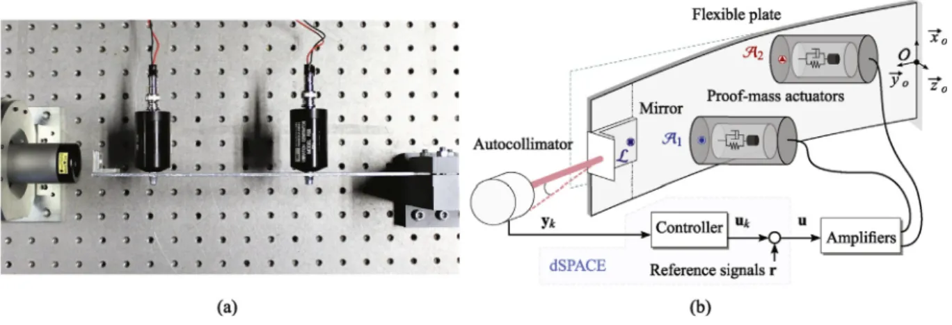
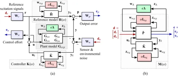
(A)denotes the maximum singular value of the real matrix A.

Fig. 1. (a) Top-down photo of the system. (b) Schematic diagram of the setup.

2. Problem formulation and system modeling

2.1. Experimental setup and control objectives

Fig. 1shows a photo and a schematic diagram of the experimental platform used in this study. The setup is mounted on an optical table and consists of autocollimator together with an aluminum cantilevered flexible plate with two proof-mass actuators (PMAs) and a mirror attached to it. The Newport CONEX-LDS autocollimator sends a laser beam that reflects of the mirror attached at the free tip of the plate and returns on a position sensor within the device. The angular deflection at the tip of the plate, corresponding to the angle between the outgoing and incoming ray, is subsequently computed down to sub

𝜇

rad resolution with a sampling frequency of 2 kHz. This angular measurement yk(t) ∈ℝis then sent to a discrete controller

implemented on a dSPACE MicroLabBox platform that computes the control voltages u_k(t) ∈ℝ2_{with a 2 kHz frequency. These}

signals are combined with the reference signals r(t) ∈ℝ2_{to form u(t) ∈ℝ}2_{. The voltages u are then used to drive the two}

Wilcoxon F5B shakers through a set of two Kepco BOP-100 amplifiers. The purpose of the controller is to alter the dynamic

response from the reference inputs r towards the angular measurements y_kin order to robustly match the response of an

adaptable reference model within a given control bandwidth. The aim of the setup is to provide a simplified model of a flexible space structure and demonstrate how the proposed design methodology can be employed for more complicated assemblies with more sensors, actuators and flexible modes. While the paper relies on this specific setup for experimental purposes, the control design process can be generalized to other space application scenarios. For example, the laser autocollimator can be replaced by a set of accelerometers or angular rate sensors while the proof-mass actuators can be replaced with piezoelectric

patches. For an overview of actuators for space applications see Ref. [26].

2.2. Model identification and mathematical modeling

The techniques presented in this paper rely on a good understanding of the main dynamics of the system in order to guar-antee worst-case behavior. In essence, to design a controller that pushes the system to the limits of performance, it is critical to first develop a system model that includes the various perturbations and uncertainties acting on the plant. This is especially important in the space industry where systems need to be designed to work without maintenance for extended periods of time and withstand different structural changes induced by thermal deformations, gyroscopic effects or equipment realignment. In this section, two models of the ESA setup are introduced: an experimental black-box model and an analytical or symbolic model based upon the physical equations of motion. The experimental model is deduced purely based on the system response to var-ious excitations. On its own, this empirical model can be used for controller design. However, this black-box representation provides no physical understanding of the dynamics of the system. As such, it is difficult to analyze and predict the changes in the overall dynamics as a result of variations in different physical parameters. To overcome such shortcomings, a second model was developed based upon the key physical principles and equations of motions. This model complemented the exper-imental one and provided deep insight into the sensitivity of the plant dynamics with respect to changes in different physical parameters. A procedure is also introduced to calibrate this analytical model and perform grey-box identification based on the experimental response.

2.2.1. Experimental model identification

Considering the plant schematic shown inFig. 1b, the black-box model identification together with the uncertainty and noise

Fig. 2. (a) Actuator voltages and measured angular deflection during the first identification experiment. Labeled time regions:○a environmental noise phase;○b first actu-ator phase; © second actuactu-ator phase. (b) Maximum sensor amplitude spectral density and cumulative root mean square (dotted line) under the influence of environmental perturbations and zero actuator signals. Labeled points:○1 first bending mode;○2 power supply electric noise.

1. the plant is driven with the voltages u=

[

u{1} u{2} ]⊺

shown inFig. 2a and the measured deflections ykwere recorded at

a sampling frequency of 2 kHz across three experiments. The time-domain identification sequence was organized in distinct phases as explained below:

(a) In the first part, labeled with○a inFig. 2a, the inputs u were kept at zero for 219samples (≈4.37 min) in order to

record in the y_kdeflection measurement the combined effect of sensor noise and environmental perturbations acting

on the flexible plate. The estimateΦ_nn(

𝜔

) of the power spectral density (PSD) of this signal was obtained at frequencies

𝜔

∈ [7

,

160]Hz using Welch’s method with a Hann window of length 219_{and 50% overlap.}

Fig. 2b shows the estimated peak amplitude spectral density1 (ASD) spectrumΦnn(

𝜔

)1/2and cumulative root-mean

square (CRMS), obtained during this phase across all experiments. The CRMS function provides a measure of the power

in a signal, up to a given frequency

𝜔

. Note that the≈6.55

𝜇

rad bias, occurring in the low frequencies below 0.1 Hz, is

due to the static misalignment between the autocollimator and the mirror attached to the plate. Above this frequency,

it can be seen that most of the power is concentrated around two key regions. Firstly, an increase of≈0.53

𝜇

rad occurs

around 10.2 Hz and corresponds to deflections around the first bending mode of the plate due to unavoidable air and ground vibrations. This bending mode will be described in detail in the subsequent section. A second significant increase

of≈0.04

𝜇

rad occurs around 50 Hz and is due to the electrical noise in the power supply of the actuator amplifiers.

For simplicity, the experimental model lumps all the different physical sources of perturbation observed in the laser

measurement ykinto a single output noise model. The measurement ykis therefore assumed to be the sum of a

“noise-free” laser displacement response y and an overall noise signal n, i.e.

y_k=y+n and n=W_nd_n with W_n∈ℝℍ∞ ; ||Wn(j

𝜔

)|| ≥ Φnn(

𝜔

)1∕2 (1)

where dnis a zero mean unit variance white noise signal and the weighting filter Wn is an upper bound on the ASD

spectrumΦnn(

𝜔

)1/2of the noise measurements.

(b) In the second and third phase (labeled○b and○c inFig. 2a), each of the actuators was driven in turn by a finite energy

stochastic signal. This random signal was obtained by passing zero mean unit variance white noise with a truncated normal distribution through a 12th order band-pass Butterworth filter with a pass-band of 5 Hz–200 Hz. The filter is

scaled such that its₂system norm (i.e. the variance of its output in response to unit white noise) is equal to the squared

RMS value desired for each of the actuator signals. The length of each excitation sequence is equal to 221_{samples for a}

total duration of≈17.5 min. At the beginning of each sequence the input signal was slowly scaled up to its nominal

value to avoid interactions with high frequency modes outside of the identification bandwidth. A similar scale down was performed at the end of each excitation sequence. Additionally a pause was inserted between these successive excitation phases to allow a decay of the flexible plate back to its resting state.

2. For each identification sequence, a Welch PSD estimateΦykyk(

𝜔

)of the output ykwas computed using a Hann window of

length 219_{and 50% overlap. This provided a frequency resolution of about 8 mHz in the spectral estimate, averaged across 8}

windowed intervals. Using the same method, the PSD estimatesΦu{1}u{1}(

𝜔

) andΦu{2}u{2}(

𝜔

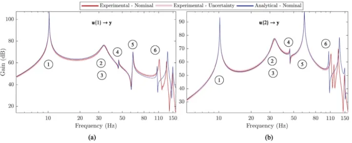
) were computed for each of the

Fig. 3. Gains of the estimated FRFs and nominal fitted plant model Gyutogether with the minimum coherence spectrum across all three identification experiments: (a) u{1}

→y channel; (b) u{2}→y channel.

input signals together with an estimateΦyku{·}(

𝜔

)of the cross power spectral density (CPSD) between each input and the

output.

3. The estimates G_yku{·}(

𝜔

)of the frequency response functions (FRF) from inputs u{·} to output y_ktogether with the

corre-sponding coherence functionsΓ_yku{·}(

𝜔

)were computed as:

Gyku{·}(

𝜔

) =

Φ_yku{·}(

𝜔

)

Φ_u{·}u{·}(

𝜔

) and Γyku{·}(

𝜔

) =

||

|Φyku{·}(

𝜔

)||| 2

Φ_u{·}u{·}(

𝜔

)Φ_ykyk(

𝜔

) (2)

The coherence function quantifies at each frequency

𝜔

, the fraction of the output PSD resulting from the input. The same

function can also be seen as a measure of the causality between the inputs and the output response [27]. Nonlinearities,

measurement noise or unwanted perturbations contribute to a reduction in the coherence spectrum. Hence, the function provides a strong indicator of the degree of uncertainty in the spectral estimate.

4. For each channel, a transfer function was fitted to the FRF results from the three experiments. The fit was performed with a

vector fitting procedure [28] using MATLAB’s tfest command. The normalized root mean squared error (NRMSE), measuring

how well the response of the model fits the estimation data, averaged around 98%. After fitting each of the channels, the transfer functions were aggregated into a global system transfer matrix and a balanced order reduction was performed. An alternative identification method, explored in this study, was to directly estimate, based on both FRFs, the overall system

transfer matrix using subspace methods and nonlinear least-squares fitting (see ssest command in MATLAB). However, this

alternative method proved to be more time consuming and the fit quality was not significantly different. Finally, the resulting

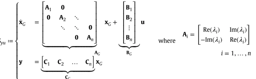
state space system G_yu∈ℝℍ1×2_∞ was put into the modal form

G_yu≔ ⎧ ⎪ ⎪ ⎪ ⎪ ⎪ ⎨ ⎪ ⎪ ⎪ ⎪ ⎪ ⎩

̇

x_G = ⎡ ⎢ ⎢ ⎢ ⎢ ⎢ ⎣ A1 0 0 A₂ ⋱ ⋱ ⋱ 0 0 An ⎤ ⎥ ⎥ ⎥ ⎥ ⎥ ⎦

⏟⏞⏞⏞⏞⏞⏞⏞⏞⏞⏞⏟⏞⏞⏞⏞⏞⏞⏞⏞⏞⏞⏟

AG x_G+ ⎡ ⎢ ⎢ ⎢ ⎢ ⎢ ⎣ B1 B₂ ⋮ Bn ⎤ ⎥ ⎥ ⎥ ⎥ ⎥ ⎦

⏟⏟⏟

BG u y = [ C1 C2 … Cn ]

⏟⏞⏞⏞⏞⏞⏞⏞⏞⏞⏞⏟⏞⏞⏞⏞⏞⏞⏞⏞⏞⏞⏟

CG x_G where A_i= [ Re(

𝜆

_i) Im(

𝜆

_i) −Im(

𝜆

i) Re(

𝜆

i) ] i=1

,

…

,

n (3)

for complex conjugate eigenvalues

𝜆

i=Re(

𝜆

i)±j Im(

𝜆

i) and Ai=

𝜆

ifor real eigenvalues. The state transformation to modal

form was performed using MATLAB’s canon command that computes a block-diagonal Schur factorization of the state matrix.

Fig. 3shows the FRFs, minimum coherence spectrum and the resulting gains of the 14th order state space model Gyu

result-ing from the previous identification procedure. It can be seen that the FRF estimates do not significantly vary across the three experiments and that the state space model reliably fits the response data in the bandwidth of interest. Furthermore, the coher-ence functions remains close to one except for frequencies near the anti-resonances and the 50 Hz power supply noise. This indicates that reliable FRF estimates were obtained using the experimental data.

The paper aims to demonstrate how the proposed control method can be applied even in the presence of significant model uncertainty. Linear Fractional Transformations (LFTs) are the one of the most widely employed means of representing uncertain

or varying parameters and other nonlinearities [29] since any rational function can be expressed as an LFT [30]. Furthermore,

at global system level. In the case of the plant considered in this paper, possible parameter variations and model inaccuracies are considered by augmenting the previously identified nominal model with an uncertainty structure. Three kinds of uncertainties are assumed to operate simultaneously:

1. Modal uncertainty. Variations in some structural parameters can lead to changes in the natural frequency and damping of

some modes. To take into account these modal uncertainties, the blocks A_iin(3)are replaced by

Â_i= [ (1+rRi

𝛿

Ri)Re(

𝜆

i) (1+rIi

𝛿

Ii)Im(

𝜆

i) −(1+r_I i

𝛿

Ii)Im(

𝜆

i) (1+rRi

𝛿

Ri)Re(

𝜆

i) ]

for complex eigenvalues and Â_i= [(1+r_R

i

𝛿

Ri)

𝜆

i] (4)

for real eigenvalues

𝜆

_i. The parameters r_R

i

,

rIi are used to set the maximum percent of variation for the real and imaginary

parts of each eigenvalue while

𝛿

_Ri

, 𝛿

_Ii ∈ [−1

,

1]are normalized real uncertainties. In this case, the new uncertain system

matrix Â, replacing the nominal one in(3), is affine in

𝛿

Ri

, 𝛿

Iiand can be expressed as the LFT:

ÂG=AG+WmL𝚫modWmR =𝚫mod

⋆

[ 0 W_mR WmL AG ] with 𝚫mod=diag ( 𝚫mod1

,

…

,

𝚫modn )

⊂

ℝnmod×nmod_and

𝚫modi i=1

,

…

,

n = ⎧ ⎪ ⎨ ⎪ ⎩ [

𝛿

RiI2

𝛿

IiI2 ]

for complex eigenvalues

𝜆

_i

𝛿

Ri for real eigenvalues

𝜆

i

(5)

where the matrices W_mL, W_mRcontaining the scaling factors r_R

i

,

rIican be computed by means of a singular value

decompo-sition (see Ref. [30] for details).

2. Additive uncertainty. Outside the identification bandwidth or around the frequencies where the coherence spectrum(2)is

low, the dynamics of the system is unknown or uncertain. These inaccuracies in the nominal system G_syswere covered using

the following additive uncertainty model: ˆ

G_yu=G_yu+W_add𝚫_add where 𝚫_add=diag(

𝛿

_add

1

, 𝛿

add2 ) and W_add= [ r_add1 r_add2 ] (6)

The Linear Time Invariant (LTI) weights r_add

•∈ℝℍ∞are used to scale at different frequencies the magnitude of the additive

normalized LTI uncertainties

𝛿

add•with

𝜎

(

𝛿

add• )

≤1.

3. Multiplicative uncertainty. Neglected dynamics or gains fluctuations in the actuators and amplifiers were modeled as mul-tiplicative uncertainties at the plant input. In this case, the new uncertain control signal û is equal to

û{•} =(1+

𝛿

_mul•r_mul•)u{•} or û= ( 𝚫mul

⋆

[ 0₂ W_mul I2 I2 ]) u with 𝚫mul=diag (

𝛿

mul1

, 𝛿

mul2 )

W_mul=diag(r_mul1

,

r_mul2)

(7)

where

𝛿

mul•are scalar normalized LTI uncertainties satisfying

𝜎

(

𝛿

mul• )

≤1 and the magnitudes of the LTI weights rdsk• ∈

ℝℍ∞quantify for different frequencies the maximum percent of relative uncertainty.

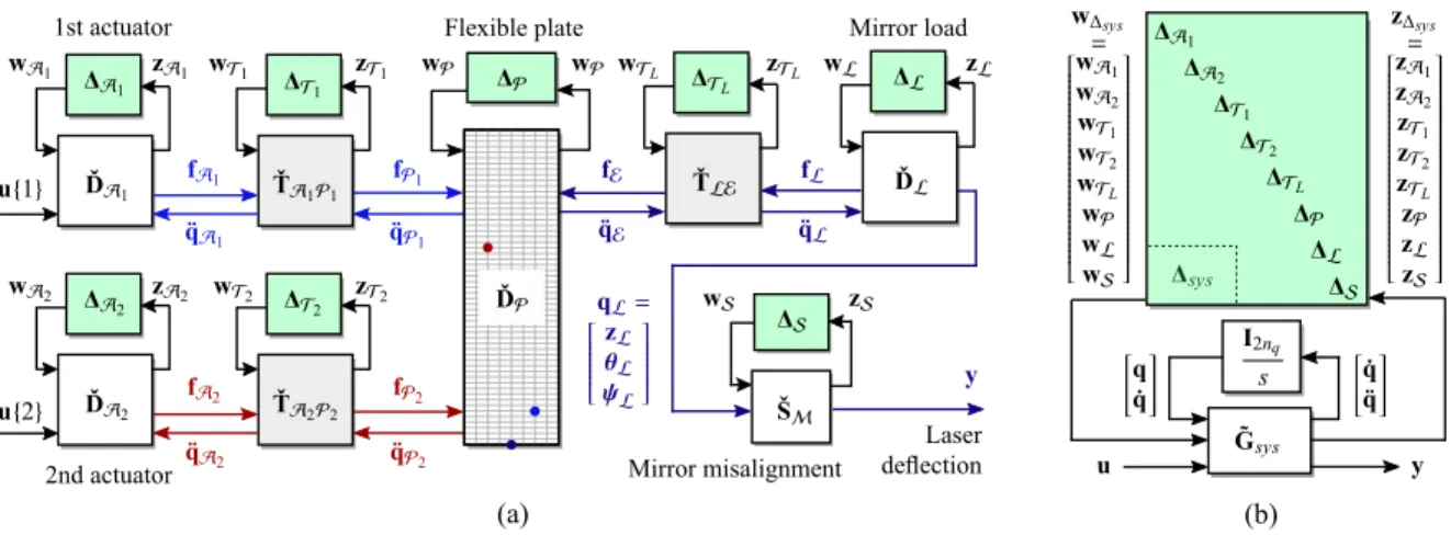
The combined effect of all these uncertainties on the input-output behavior of the system can be studied by aggregating them into the following global uncertainty model:

(8)

Fig. 4a highlights this LFT structure of the global uncertain model while fig. b shows the separate effects of each type of uncer-tainty on the gains of the transfer function from the input u{2} to the output y.

2.2.2. Analytical modeling

In order to extract a symbolic representation of the dynamics, the plant is modeled as the interconnection of a finite ele-ment model (FEM) of the flexible cantilevered plate, two proof-mass actuators and the mirror load. Each of these subsystems is described below and afterwards assembled into a global structure. The numerical values and range of variation of the various

system parameters that are used in this section are give inTable 1. These values were either measured directly, provided in the

Fig. 4. (a) Internal structure of the uncertain experimental model of the plant. (b) The effects of different sets of uncertainties on the gains of the channel u{2}→y.

Table 1

Nominal parameter values of the overall system.

Subsystem Parameter Description Value & Uncertainty

Flexible plate 𝜌 density 2692 kg m−3

E Young’s modulus 69 GPa

𝜈 Poisson’s ratio 0.33 l length 30 cm w width 4 cm h thickness 3 mm 𝛽M,𝛽K damping coefficients 0.1, 10−5 ⃖⃖⃖⃖⃖⃖⃖⃗

1 location 1st actuator node [-1 25 0]⊺cm

⃖⃖⃖⃖⃖⃖⃖⃗

2 location 2nd actuator node [1 10.5 0]⊺cm

⃖⃖⃖⃖⃖⃗

 location mirror load node [0 28 0]⊺cm

Actuators m_• mass of the moving mass 23.5 g

mc• mass of the casing 96.5 g

Jc• moment of inertia of the outer casing in CoM frame

( •;⃗xa•, ⃗ya•,⃗za• ) [114.04 114.04 ] mg m2 a_• gain 1.5 N V−1 k• stiffness 26 N m−1 c• damping 10 N s m−1

r_•• attachment point location relative to outer casing CoM, i.e.⃖⃖⃖⃖⃖⃖⃖⃖⃖⃗••

[

0 0 −1.35

]⊺ cm

Mirror m_ mass 24.3 g

J_ moment of inertia in CoM frame( ;⃗xl, ⃗yl,⃗zl

) [1.968

56.266

]

mg m2 r_ attachment point location relative to CoM i.e.⃖⃖⃖⃖⃗

[

0 −1.44 −0.81

]⊺ cm r_𝜓

, rz_ misalignment parameters between the laser beam and the reflecting surface 1e-3, 5e-3

Note: components of the location vectors are given in the inertial frame( ;⃗xo, ⃗yo,⃗zo

)

when the plate is at rest.

1. Flexible plate model. The flexible plate was modeled as a Kirchhoff thin plate subdivided into the assembly of

intercon-nected four-node rectangular plate elements shown inFig. 5a. Each rectangle element has a side length of 5 mm at rest. The

inertial reference frame( ;

⃗

x_o

, ⃗

y_o

,⃗

z_o), visible inFigs. 1 and 5a, is fixed to the node at the center of edge anchored to the base structure. Attached to each of the unclamped nodes is a frame

(

•;

⃗

x•

, ⃗

y•

,⃗

z• )

coincident in the rest state with

the inertial frame. Each node has three degrees of freedom q_

•= [ z_ •

𝜽

•

𝝍

• ]⊺ where z_ • is the displacement along the

⃗

z_

•axis,

𝜽

•the rotation angle around the

⃗

x•axis and

𝝍

•the rotation angle around the

⃗

y•axis. Rotations

around the

⃗

z_•axis are not considered. After grouping the node displacements into an overall displacement vector q_, the

linearized dynamics of the flexible plate becomes

M_q

̈

_+C_q

̇

_+K_q_ =f_ with C_ =

𝛽

MM+

𝛽

KK and q(t) ∈ℝ1512 (9)

where f_ are the generalized forces acting on every node coordinate of the plate. The state q_ has a dimension of 1512

since the plate is discretized into 9×57 nodes, each with 3 coordinates and 9 of the nodes are in clamped condition. The

mass and stiffness matrices M_and K_depend on structural properties of the plate given inTable 1. In-depth details on the

Fig. 5. (a) Finite element model of the flexible plate together with corresponding coordinate frames and illustration of the four node plate element. (b) Diagram of the first

proof-mass actuator model in unclamped configuration illustrating the displacements z1and zc1relative to the rest state (dashed lines).

phenomenon to model physically, the classical (or Rayleigh) damping matrix C_ is defined in terms of two uncertain real

scalars

𝛽

_Mand

𝛽

_K. The model assumes that each of the two PMAs both as well as the mirror load connect to the flexible plate

attachment nodes labeled with(_•;

⃗

x_p•

, ⃗

y_p•

,⃗

z_p•)and( ;

⃗

x_e

, ⃗

y_e

,⃗

z_e)inFig. 5a. The plate’s equations of motion given in(9)

can be rewritten in terms of input forces and output accelerations at the attachment nodes as

[

̈

q⊺_ q

̈

⊺_ 1 q

̈

⊺ 2 ]⊺ =D_[f⊺_ f⊺_ 1 f ⊺ 2 ]⊺ with D_ =𝚫_

⋆ ́

D_ ∈ℝℍ9×9_∞ (10)

where the uncertain block diagonal matrix𝚫_ isolates the uncertain part of the damping coefficients

𝛼

Mand

𝛼

K.

2. Mirror load model. The mirror used to reflect the laser beam is fixed to the plate using an aluminum L-shape (seeFig. 1),

that significantly increases the stiffness of the plate region directly underneath. For simplicity, the mirror, together with the

L-shape and the whole width of the plate under it, are modeled as a single rigid body load of mass m_. This combined static

load connects to the plate model at the frame( ;

⃗

xe

, ⃗

ye

,⃗

ze )

corresponding to the central node at the end of the flexible part of the plate. Coincident with this attachment frame is a body frame( ;

⃗

x_l

, ⃗

y_l

,⃗

z_l)fixed at the center-of-mass of the load.

The load was coupled to the plate dynamics by first translating plate accelerationsq

̈

_=

[

̈

z_

̈𝜽

_

̈𝝍

_ ]⊺ of the attachment node frame( ;

⃗

xe

, ⃗

ye

,⃗

ze ) to accelerationsq

̈

_= [

̈

z_

̈𝜽

_

̈𝝍

_ ]⊺

of the load body frame( ;

⃗

xl

, ⃗

yl

,⃗

zl )

. Multiplying these

body frame accelerations by the dynamic model of the load results in generalized reaction forces f_in the load body frame.

These forces were subsequently translated to reaction forces f_in the attachment node frame in order to couple the plate

and load dynamics. The linearized dynamical equations can therefore be expressed as

⎧ ⎪ ⎪ ⎨ ⎪ ⎪ ⎩ [

̈

q_ f_ ] = [  (r_) 0 0  (r_)⊺ ] [

̈

q_ f_ ] =𝚫_L

⋆

Tˇ_ [

̈

q_ f_ ] f_= [ m_ 0 0 J_ ]

̈

q_=𝚫_

⋆ ́

D_q

̈

_ with  (r_) =S⊺  [ I3 [ r_]_× 3 I₃ ] S_ S_ = [ 03×2 I3 03×1 ]⊺ [ r_]_×= ⎡ ⎢ ⎢ ⎢ ⎣ 0 −r_{3} r_{2} r_{3} 0 −r_{1} −r_{2} r_{1} 0 ⎤ ⎥ ⎥ ⎥ ⎦ (11)

where r_∈ℝ3_{are the coordinates of the attachment pointrelative to the mirror CoM, i.e.}

⃖⃖⃖⃖⃗

_{expressed in the inertial}

frame( ;

⃗

x_o

, ⃗

y_o

,⃗

z_o). m_and J_are the mass and the 2×2 moment inertia tensor of the mirror in the body frame. The matrix

J_is only 2×2 since the load body frame( ;

⃗

x_l

, ⃗

y_l

,⃗

z_l)is always coincident with the attachment node frame( ;

⃗

x_e

, ⃗

y_e

,⃗

z_e)

and rotations around the

⃗

z_eare not considered in the flexible plate model. The blocks𝚫_

Land𝚫capture the uncertainties

on the geometric and inertial parameters of the mirror load. The selection matrix S_ is needed to truncate the kinematic

transport matrix

[

I₃ [r_]_× O3I3

]

since each plate node only has three coordinates (z_

•,

𝜽

•and

𝜑

•) instead of the usual

3. Mirror/laser misalignment model. The noise free laser measurement y was considered to be almost equal to the pitch angle

𝜽

of the mirror around its

⃗

xaxis. Because of small deformations in the mirror surface as well as the inevitable misalignment

between the laser beam and the reflecting mirror, the measurement y is also influenced by the axial displacement z_and the

roll angle

𝝍

_of the mirror load. In order to take into account these effects, the following uncertain model was introduced

(12)

where

𝛿

_𝜓



, 𝛿

z_∈ [−1

,

1]are real parametric uncertainties and r𝜓_

,

rz_∈ℝare used to set the maximum degree of expected

coupling.

4. Proof-mass actuator model.Fig. 5b illustrates the model of the first PMA. This actuator was modeled as a hollow cylinder

of mass m_c1and enclosing a point mass m₁. This small mass attaches to the outside casing with a viscoelastic connection of

stiffness k₁and damping c₁. The body frame(₁;x

⃗

_a1

, ⃗

y_a1

,⃗

z_a1)is fixed to the center-of-mass of the outside shell. Additionally, this frame forms a rigid connection with the plate frame(₁;

⃗

x_p1

, ⃗

y_p1

,⃗

z_p1)corresponding to node directly underneath the actuator (seeFig. 5a for clarity). Since rotations aroundz

⃖⃖⃖⃗

_p1axis are ignored in flexible plate model and(₁;

⃗

x_p1

, ⃗

y_p1

,⃗

z_p1)

remains coincident with(1;

⃗

xa1

, ⃗

ya1

,⃗

za1 )

, the moment of inertia tensor of the shell in the body frame Jc1is only 2×2. The

control signal u{1} generates a magnetic force of magnitude a₁u{1} in the voice coil that is applied in opposite directions

to both the shell and the small mass. In the case when the actuator is not clamped to a supporting structure, this force

produces a displacement z1of the small mass and a displacement zc1of the cylindrical shell casing in an inertial reference

frame coincident with(₁;

⃗

x_a1

, ⃗

y_a1

,⃗

z_a1)at rest. In this case, the translational dynamics is described by the following set of equations: [ m₁ 0 0 mc1 ] [

̈

z₁

̈

zc1 ] + [ c₁ −c₁ −c1 c1 ] [

̇

z₁

̇

zc1 ] + [ k₁ −k₁ −k1 k1 ] [ z₁ zc1 ] = [ a₁ −a1 ] u{1} + [ 0 1 ] fzc1 (13)

where fzc1is an external axial force applied to the enclosing shell. When the actuator is clamped to the beam, the previous

set of equations need to be slightly adapted. Firstly, as performed for the mirror load in(11), the static inertia of the shell

casing was added to the plate node₁. Secondly. the axial acceleration of the shell becomes equal to that of the supporting

node, i.e.z

̈

_c1=q

̈

_1{1}. In this case, the equations for the clamped PMA are

[

̈

q_ 1 f_1 ] = [  (r_ 11) 0 0  (r_11)⊺ ]

⏟⏞⏞⏞⏞⏞⏞⏞⏞⏞⏞⏞⏞⏞⏞⏞⏟⏞⏞⏞⏞⏞⏞⏞⏞⏞⏞⏞⏞⏞⏞⏞⏟

T_11=𝚫_1⋆̌T_11 [

̈

q_ 1 f_1 ] and ⎧ ⎪ ⎪ ⎪ ⎪ ⎨ ⎪ ⎪ ⎪ ⎪ ⎩ f_ 1 = [ m_c1 0 0 J_c1 ]

̈

q_ 1+ ⎡ ⎢ ⎢ ⎢ ⎣ 1 0 0 ⎤ ⎥ ⎥ ⎥ ⎦ f_pma1 fpma1 =c1e

̇

z1+k1ez1+a1u{1} ez1 =z1−q1{1}

̈

z1 = −m−11 fpma1 (14) where r_

11are the coordinates of the attachment point1relative to outer casing CoM1, the function (·)constructs

the truncated kinematic transport matrix as defined in(11)and𝚫_1captures the uncertainties in the location of the center

of mass. In terms of input-output behavior, the same PMA dynamics can also be expressed as the following transfer function:

f_1 =D_1 [ u{1}

̈

q_1 ] with D_1=𝚫_1

⋆ ́

D_1∈ℝℍ3×4_∞ (15)

where𝚫_1combines the block𝚫_1 and the uncertainty in the other actuator parameters. The dynamical equations of the

second PMA are almost completely similar to eqs.(13)–(15), except for changes in each of the indices (for example₁

becomes₂and u{1} becomes u{2}).

The subcomponent models defined in eqs.(9), (11) and (14)were subsequently combined into the following global model

mapping actuator inputs u to laser displacement y:

Fig. 6. (a) Block diagram of the uncertain plant together with the various subcomponents written in LFT form. Note: the grid on theD́_flexible plate block corresponds to the FEM node grid and the colored circles indicate the various attachment nodes. (b) Equivalent global LFT form.

where q= [ q⊺  z1 z2 ]⊺ ; q(t) ∈ℝnq_{; n}

q=1514 combines the node displacements q of the flexible plane with those of

the proof-masses z₁, z₂. The matrices

,



,



,



,

are the uncertain mass, damping, stiffness, input and output matrices. An

equivalent representation of the same dynamical model can be deduced by combining each of the subsystem LFTs from eqs.(10)

to (12) and (15)into the following global LFT representation:

G_sys=𝚫_sys

⋆

I2nq

s

⋆

∼

G_sys with 𝚫_sys=diag

(

𝚫1

,

𝚫2

,

𝚫1

,

𝚫2

,

𝚫L

,

𝚫

,

𝚫

,

𝚫

)

(17)

Fig. 6illustrates the internal structure of this overall LFT model and the interconnections between the various subcomponents.

This block diagram LFT representation of G_sysoffers some advantages over the system level description given in(16). Firstly,

this method of assembly can be more versatile since the different component blocks can be easily interchanged with others

from an existing library (see Ref. [33] for an example). Secondly, since the block uncertainty is already isolated at the

compo-nent level, a low order global uncertainty block𝚫_syscan be easily constructed by just concatenating the individual uncertainty

blocks. In the system level description from(16), care must be taken to ensure that the uncertain matrices are properly

fac-torized to avoid unwanted repetitions of the uncertain parameters. However, the first representation also comes with some distinct advantages. In particular, the first representation was used to compute the nominal mass-normalized modal matrix

𝚽 =[

𝝋

1

𝝋

2 …

𝝋

nq

]

∈ℝnq×nq _{of the overall mechanical system. This matrix was calculated by assuming no damping}

and nominal values for the mass and stiffness matrices and satisfies

𝚽⊺_{M𝚽 =I} nq ; ( K−

𝜔

2_iM )

𝝋

i=0 for i=1

,

…

,

nq ; 𝚽⊺K𝚽 =diag (

𝜔

2 1

,

…

, 𝜔

2 nq ) (18)

where

𝜔

_iis the modal frequency associated with every mode shape

𝝋

_i. The matrixΦserves two primary purposes:

(a) Mode shape visualization. Each mode shapes

𝝋

_ican be visualized in order to get insight into the various interactions

between the subcomponents and the different ways the structure can vibrate at the resonant frequencies.

(b) System order reduction by modal truncation. It can be seen from(16)that the order of Gsysis equal to 2nq=3028.

Such a high order system would introduce significant numerical difficulties in any subsequent analysis. For this

rea-son, the modal matrix𝚽was used to perform an order reduction. In this case, the generalized displacements q can be

expressed in terms of the modal coordinates

𝜼

(t) ∈ℝnq_{as q= Φ}

𝜂

_{. From the modal orthogonality condition in(18)it}

fol-lows that𝚽−1=𝚽⊺M and therefore

𝜼

=𝚽−1q=𝚽⊺Mq. Consider now a partitioning𝚽 =[_{𝚽r 𝚽t}]and

𝜼

=

[

𝜼

⊺r

𝜼

⊺t

]⊺

where𝚽_r∈ℝnq×nr_{contains the n}

r=12 modal vectors to be retained andΦtthose that will be truncated. The original

displacement vector q= Φ_r

𝜂

_r+ Φ_t

𝜂

_tfrom(16)is therefore approximated with q≈ Φ_r

𝜂

_r. Using again the modal

orthogo-nality condition𝚽⊺_rM𝚽r=Inrit follows that𝚽 +

r =𝚽

⊺

rM is a generalized left inverse ofΦri.e.𝚽+r𝚽r=Inrand therefore

𝜼

r≈ ( 𝚽+ rq=𝚽 ⊺ rMq )

. In this case,(16)andFig. 6a can be updated to reflect the newly reduced order system by replacing

the integrator relationship on the state[q⊺ q

̇

⊺

]⊺

Fig. 7. (a) Interconnection used for grey-box identification. (b) Solid lines: upper bounds computed using𝜇-analysis on the gains of the u{2}→y channel for±25% variation around the nominal values of various physical parameters. Dashed lines: gains for different values of the corresponding uncertain parameter.

(19)

The system order is therefore reduced from 2nq=3028 to 2nr=24. The reduction procedure is equivalent to rewriting

G_sysfrom(16)as

(20)

However, the integrator reduction method proposed in(19)is slightly more advantageous, since it can be directly applied

to the block diagram LFT representation from(17), also shown inFig. 6. The truncation errors induced by this model

reduction can be included into an additional additive uncertainty model as performed in Ref. [16].

2.2.3. Grey-box identification

The reduced order analytical model Gsys=𝚫sys

⋆

Gˇsysdetailed in(19)contains k real uncertain parameters

𝛿

p•in the block

diagonal block𝚫_sys. In order to calibrate the nominal values of these various physical parameters, a grey-box identification

procedure was used. The proposed method relies on the interconnection shown inFig. 7a between Gsysand the uncertain

exper-imental model Gexp=

𝜖

𝚫

⋆

Gˇexpfrom(8), where the parameter

𝜖

≤1 was introduced to scale the set of normalized experimental

uncertainty. The idea is to search for a set of parameter values for the uncertainty block𝚫_systhat minimizes the worst-case

weighted additive error between the two models across the reduced subset of experimental uncertainties

𝜖

𝚫. This takes the

form of the following optimization procedure: mininimize

𝚫sys

𝛾

s.t. sup

𝚫 ;𝜎(𝚫)≤1

W_e[(

𝜖

𝚫

⋆

Gˇ_exp)−(𝚫sys

⋆

Gˇsys )]

W_{r ∞}≤

𝛾

(21)

where the weighting function We was fixed to a unit gain second order band-pass Butterworth filter with a pass-band of

5 Hz–80 Hz. The purpose of this weight is to put more emphasis on the model errors within the control bandwidth. The other

weight W_rcan be used, in the general case, to optimize the model error for a specific class of input signals. For simplicity, this

weight was fixed to Wr=I2in this study and the value

𝜖

=0.05 was selected to account for only 5% of the total experimental

uncertainty𝚫.

The optimization problem in(21)was treated as a robust synthesis problem involving the structured block𝚫_sys. This class

of problems is known to be NP-hard even when the controller to be designed is unstructured. Nevertheless, powerful heuristic methods, have been developed to help deal with such problems. In this work, the heuristic method of choice was the

Ref. [35] can directly tackle the minimization problem expressed in(21). However, in this work a slightly simplified version

was optimized. In this case, the worst case error is not calculated across all𝚫;

𝜎

(𝚫) ≤1 but rather across a smaller subset of

random samples. This multi-model approach resulted in a faster tuning process but also required a subsequent

𝜇

analysis to

verify if the_∞norm condition was satisfied across the larger set. If any uncertainty combination was found to invalidate the

norm requirement using the

𝜇

analysis, then that particular uncertainty was added to the collection of random samples. The

optimization process was then repeated until no other uncertainty could be found or a finite number of iterations was reached.

The nominal identified nominal values of the various parameters are provided inTable 1.

Fig. 8shows the result of this tuning procedure by comparing the gains u{•}→y of the tuned nominal analytical model𝚫_sys

⋆

Gˇ_systo the gains of the uncertain experimental model(

𝜖

𝚫)

⋆

Gˇ_exp. It can be seen that the mathematical model reliably fits

the experimental model in the control bandwidth of interest of 5–80 Hz. The expected model discrepancy occurring at high frequency most likely occurs due to deviations from the ideal Kirchhoff plate model, nonlinear damping effects or actuator dynamics. However, the analytical model is sufficient to provide a great deal of physical insight into the system dynamics.

For example, the first six mode shapes𝚽i; i=1,…, 6 were calculated up to a frequency of 110 Hz using(18). The mode

shapes labeled○1 to○6 are illustrated inFig. 9and their respective natural frequency is indicated inFig. 8. The newly fitted

analytical model also enabled the possibility to perform detailed parametric sensitivity analysis such as the one shown inFig. 8.

Here, several physical parameters were varied within a±25% range around their nominal values and an upper bound on the

transfer u{2}→y was computed using standard

𝜇

analysis. In this way, the impact of each parameter variation can be accurately

predicted across the frequency range. For example, modifying the mass m_of the mirror load corresponds to a frequency shift

of the first bending mode. Similarly, changing the damping coefficient c2of the second PMA, modifies both the damping of

the corresponding actuator mode and the damping of the second bending mode. On the other hand, modifying the offset rz=

r_

11{3} =r22{3} between the center of mass of the two PMAs and the plate attachment nodes causes a shift in both

frequency and damping for all the modes above 40 Hz due to the change in the torsional moment of inertia.

3. Controller design and limits of performance

3.1. Control architecture and synthesis methodology

The purpose of the controller K is to produce an adequate control signal uk=Kykthat meets the following requirements:

R1. Robust stability: the closed loop shall be stable across all the uncertainties𝚫modeled using(8).

R2. Robust performance: the control signals and the model error between the experimental plant and an adaptable

refer-ence model H must be minimized and guaranteed to be below a certain specified level for a restricted subset of uncertainties

𝜖

𝚫with

𝜖

∈ [0

,

1].

To ensure such requirements, the controller was optimized following _∞∕

𝜇

design practices, by first assembling the

weighted interconnection shown inFig. 10. This interconnection is composed of the following blocks:

1. Uncertain plant model G_sys: For controller synthesis, either the experimental model G_exp=𝚫

⋆

[

GzwGzu

G_ywG_yu

]

from(8)or the

reduced physical model Gsys=𝚫sys

⋆

Gˇsysfrom(19)can be used. The choice depends on the particular design objectives.

For example, the analytical model provides the user with virtual access to any physical signal in the overall plant. This can be of considerable advantage since one can rely on these virtual measurements to monitor and possibly manipulate signals for which no sensor is available. On the other hand, the experimental model can be readily derived for a general flexible structure with a more complex shape. Since the aim of the paper is to outline a general control methodology for dynamic

reshaping, the choice was made to use the experimental model G_expfor control design and rely on the analytical model G_sys

for a more in-depth worst-case analysis.

2. Disturbance weights W_nand W_r: The measurement noise weight W_nwas introduced in(1)and is used to model the upper

bound on the expected ASD spectrum of the experimental closed-loop noise measurements. Similarly, the filter W_rspecifies

the upper bound on the ASD of the closed-loop reference signals r. The reference inputs r used in the closed loop experiments

were chosen to be the same as the signals u used during the experimental identification phase (see section2.2.1andFig. 2a).

Therefore, W_rwas chosen as a scaled 4th order band-pass Butterworth filter with a pass-band of 5 Hz–200 Hz and the same

amplitude as the one used to color the white noise open loop identification signals.

3. Adaptable reference model H(

𝛼

): This model represents the target dynamic response for the close-loop plant and is

parame-terized in terms of a normalized scheduling parameter

𝛼

∈ℝ ; |

𝛼

| ≤1. In this paper, H(

𝛼

) ∈ℝℍ1×2_∞ is based on the nominal

open loop plant G_yuexpressed in canonical modal from in(3). The difference is that for H(

𝛼

), the pairs of complex eigenvalues

𝜆

iare parameterized in terms of a

𝛼

as

𝜆

i=fi(

𝛼

)±jgi(

𝛼

). In the general case, the functions fi(

𝛼

)

,

gi(

𝛼

) ∶ℝ → ℝcan be any

following LFT:

(22)

where n_H =6 is the minimal number of repetitions of

𝛼

in the LFT description, m=4 is the number of poles up to 70 Hz

in Gyuand the matrices Biand Ciare the ones from(3).Fig. 11shows the gains and pole maps of H for different values of

𝛼

compared to the open loop plant G_yu. It can be seen that for

𝛼

= −1, the damping coefficients of the PMA modes around

35 Hz and the second bending mode around 63 Hz are increased by over an order of magnitude compared to the open loop.

When

𝛼

=1, the damping of the first open loop bending mode around 10 Hz is increased by two orders of magnitude. At the

same time, the natural frequency of this flexible mode is raised up to 14 Hz. The torsional mode around 45 Hz is kept at the

open loop values. The reason why H(

𝛼

) was chosen to have this dependency on

𝛼

was to demonstrate that the controller can

distinctly and selectively change the structural behavior of the plant at different frequencies. This particular value for H was

also selected based on the limits of performance analysis detailed in section3.2.

4. Performance weights W_uand W_p: The purpose of the weight W_u=w−1

u I2 ;wu∈ℝℍ∞is to impose a desired closed loop

upper bound of |w_u(j

𝜔

)| on the worst-case ASD of the actuator signals u at different frequencies

𝜔

. In this way, the

specifica-tion on the maximum actuator RMS can be guaranteed across any frequency band since the RMS is equal to the square root of the area under the PSD curve. For the specific actuator used in the study, the RMS of the input voltage must stay below

0.1 V to avoid damage to the coil. Therefore wuwas fixed to wu=5.0·10−3to ensure a bound of 5×10−3V∕

√

Hz on the

ASD and a maximum RMS of 0.1 V up to 200 Hz. Likewise, the weight Wp=w−1p ; wp∈ℝℍ∞is used to specify the desired

upper bound |w_p(j

𝜔

)| on the ASD of the error p between the output y_hof the reference model H and the output y of the plant

model G_exp. In this case w_pwas chosen as a 4th order bandstop filter with maximum tracking error ASD of 50

𝜇

rad∕√Hz in

the 7 Hz–70 Hz stopband and a maximum of 500

𝜇

rad∕√Hz outside of it.

To ensure that the requirements are not conflicting or too conservative, the values for the performance weights Wuand Wp

were chosen after understanding some of the fundamental limits of performance imposed by the control architecture. Details

about this analysis are provided in section3.2.

5. Structured adaptable controller K(

𝛼

): To facilitate the implementation of the control law but also provide sufficient

adapt-ability to changes in the reference model H(

𝛼

), the following affine structure K(

𝛼

) is imposed on the controller:

(23) where A_K0, A_K1, B_K0, B_K0, C_K0, C_K0, D_K0, D_K0 are real matrices of appropriate dimension. The controller order n_qk=6, the

number of repetitions nK=6 of the scheduling parameter

𝛼

and the initial values for the controller matrices were chosen

after following the iterative procedure detailed in Ref. [16]. To speed up the subsequent optimization, the matrices A_K0, A_K1

are constrained to be tridiagonal. For ensuing experiments, the controller is implemented in discrete-time following a Tustin

transformation with a sampling time T=0.5 ms synchronized with the 2 kHz sampling frequency of the autocollimator

sensor. In this case, each of the integrators1

sin(23)is replaced with

T

2 1+z−1

1−z−1, where z−1is the unit delay. In compact notation this is equivalent to:

(24)

Using the previous component definitions, the closed-loop relationship between the various input and output signals shown inFig. 10and the controller K can be determined. In the open loop case, the following mapping exists between the input and

output signals shown inFig. 10:

Fig. 8. Comparison between the gains of the experimental and analytical models: (a) u{1}→y channel; (b) u{2}→y channel. (Note: the region shaded in corresponds to the scaled uncertainty set𝜖𝚫sysconsidered during the grey-box fitting optimization(21).).

Closing the loop with the controller K(

𝛼

) such that u_k=K(

𝛼

)y_kresults in the following new mapping between the signals:

(26)

where S(

𝛼

) =[I+G_yuK(

𝛼

)]−1denotes the Output Sensitivity Function and the dependency on

𝛼

of K, H and S was omitted for

clarity. After closing the uncertainty channels with the scaled uncertainty

𝜖

𝚫 ;

𝜖

∈ [0

,

1], i.e. w_Δ=(

𝜖

𝚫)z_Δthe controller design problem can be stated as the following optimization:

mininimize ˇ K∈𝕂

𝛾

s.t. 𝚫 ;𝜎(𝚫)≤1;|sup 𝛼|≤1

𝜖

𝚫

⋆

(

𝛼

InH )

⋆ ̌

P

⋆

Kˇ

⋆

(

𝛼

InK )

⏟⏞⏞⏞⏞⏞⏞⏞⏞⏞⏞⏞⏞⏞⏞⏞⏟⏞⏞⏞⏞⏞⏞⏞⏞⏞⏞⏞⏞⏞⏞⏞⏟

M(𝛼) _∞ ≤

𝛾

(27)

Any controller for which

𝛾 <

1 satisfies the robust performance and stability requirements. More precisely, it represents a

robust and structured Linear Parameter Varying (LPV) synthesis problem. However, in this work the time-varying aspect of the

parameter

𝛼

is not explicitly taken into account and the constraints on the L₂system gain in(27)are only enforced for fixed

values of

𝛼

. Therefore, the optimization is comparable in complexity to the grey-box fitting method proposed in(27)and the

same set of nonsmooth_∞tools were used to address the problem. In order to improve readability of the paper, additional

details about all the various steps and heuristics needed to solve(27)were suppressed. A complete explanation of the process

used to obtain the structured LPV controller ˇK∈𝕂using non-smooth_∞tools can be found in Refs. [16,17,36]. In the case of

the optimization given in(27), a controller ˇK was found to achieve a performance level of

𝛾

=0.989.Fig. 12shows the gains and

pole map of this controller K(

𝛼

) =Kˇ

⋆

(

𝛼

I_n

K

)

for different values of the scheduling parameter

𝛼

∈ [−1

,

1].

It is important to understand the shape of the resulting controller and also the trade-offs involved in the overall control design. A detailed analysis of the limits of closed-loop performance is therefore provided in the following subsection.

3.2. Limits of performance and trade-off analysis

During the requirements specification phase, it is important to have an intuition about what can be achieved using feed-back, subject to the various constraints imposed by available bandwidth, actuator limitations, environmental noise and model uncertainty. This sort of understanding about the limits of performance can simplify the process of selecting the desired perfor-mance requirements and the corresponding weights prior to the controller tuning. Additionally, before any experimentation, it is important to understand the mechanisms of action of the controller and cross-check the results returned by automatic syn-thesis tools. The goal of this section is to show how this trade-off analysis was performed prior to any control synsyn-thesis and how

the results can be used to explain the gains of the synthesized controller shown inFig. 12.

For any stabilizing controller K(

𝛼

), the sensitivity S(

𝛼

) =[I+G_yuK(

𝛼

)]−1is subject to the following types of constraints for all fixed values of

𝛼

∈ [−1

,

1]:

Fig. 9. Nominal mode shapes of the undamped analytical model up to 110 Hz numbered inFig. 8:○1 1st bending mode;○2 1st actuator mode (in-phase proof-mass displacements);○3 2nd actuator mode (out-of-phase proof-mass displacements);○4 1st torsional mode;○5 2nd bending mode;○6 2nd torsional mode.

Fig. 10. (a) System architecture used for controller synthesis and worst-case analysis. (b) Equivalent standard form of the interconnection.

1. Analytical constraints. Bode’s Sensitivity Integral also known as the waterbed effect can be seen as a conservation law valid

for all stabilizing controllers [37]. Briefly, this constraint states that if the controller pushes on the sensitivity function S at

one frequency it automatically increases its value at some other frequencies by the same amount. More precisely, consider

an arbitrary MIMO plant G_yuand a controller K compatible in size such that each of the entries in the open loop transfer

matrix G_yuK are rational functions with at least two more poles than zeros. In this case, if the closed loop is stable, then the

singular values

𝜎

iof S with i=1,…, n𝜎satisfy [38]: n_𝜎 ∑ i=1 ∫ ∞ 0 log

𝜎

i [ S(j

𝜔

)]d

𝜔

=

𝜋

Np ∑ i=1 Re(pi) (28)

where p_irepresents the N_pright-hand plane poles. The assumption on the excess number of poles is not restrictive for the

type of plants G_yuconsidered in this study, namely flexible structures. This is because both actuators and sensors have a