Towards a demonstrator for autonomous object detection on board Gaia

HAL Id: tel-00340279

https://tel.archives-ouvertes.fr/tel-00340279v2

Submitted on 21 Nov 2008

HAL is a multi-disciplinary open access

archive for the deposit and dissemination of

sci-entific research documents, whether they are

pub-lished or not. The documents may come from

teaching and research institutions in France or

abroad, or from public or private research centers.

L’archive ouverte pluridisciplinaire HAL, est

destinée au dépôt et à la diffusion de documents

scientifiques de niveau recherche, publiés ou non,

émanant des établissements d’enseignement et de

recherche français ou étrangers, des laboratoires

publics ou privés.

Towards a demonstrator for autonomous object

detection on board Gaia

Shan Mignot

To cite this version:

Shan Mignot. Towards a demonstrator for autonomous object detection on board Gaia. Signal and

Image processing. Observatoire de Paris, 2008. English. �tel-00340279v2�

OBSERVATOIRE DE PARIS

´

ECOLE DOCTORALE

ASTRONOMIE ET ASTROPHYSIQUE D’ˆ

ILE-DE-FRANCE

Thesis

ASTRONOMY AND ASTROPHYSICS

Instrumentation

Shan Mignot

Towards a demonstrator for autonomous

object detection on board Gaia

(Vers un demonstrateur pour la d´

etection

autonome des objets `

a bord de Gaia)

Thesis directed by Jean Lacroix then Albert Bijaoui

Presented on January 10th 2008 to a jury composed of:

Ana G´omez G ´EPI - Observatoire de Paris President

Bertrand Granado ETIS - ENSEA Reviewer

Michael Perryman ESTEC - Agence Spatiale Europ´eenne Reviewer

Daniel Gaff´e LEAT - Universit´e de Nice Sophia-Antipolis Examiner

Michel Paindavoine LE2I - Universit´e de Bourgogne Examiner

Albert Bijaoui Cassiop´ee - Observatoire de la Cˆote d’Azur Director

Gregory Flandin EADS Astrium SAS Guest

Jean Lacroix LPMA - Universit´e Paris 6 Guest

Acknowledgements

The journey to the stars is a long one. If the poet may with one swift movement of his imagination

sweep the reader off his feet to embark at their summons on a voyage to the blinking stars, for the

multitude, the path remains undecipherable. Many an intriguing stratagems have been devised by

generations of men yearning for such freedom and, alas, of those who have succeeded little remains

but awe for their genius or for their folly. By no means do we hope to compare with them. Instead,

with the sand at our feet to the stars above our heads, we venture to construct a ladder, grain per

grain, and with infinite patience and method, eventually, step by step. May the readers forgive the

means, overlook the ticking of the inflexible clock and bear with us long enough to either discard

our laborious undertaking with evidence or to contribute their own grain. . . for such an endeavour

cannot be a solitary one.

And, indeed, a solitary one it has not been. From the start, the buzz of the contradictors and of

the collaborators was heard surrounding our molehill. Certainly, the improbable balance in which it

now stands owes much to the varied views of the scientists, of the engineers, of the agencies as of

industry. Pray, accept our gratitude for doubts, good counsels, militant beliefs, patient contributions,

precise criticisms have shaped the edifice, sometimes like a wind bringing down feverish protrusions,

sometimes like a lever. Of all, special praise must be given to my directors and my proofreaders,

and among them to Philippe Laporte who has not only groped for viable solutions in the realm of

hardware in our company, but has also bravely ventured in inspecting every single portion of this

text where many dangers lay in hidding.

Family, friends and our sweetheart have also played a decisive role. Some with earthly, and others

with not so earthly means. Let them not be forgotten, for if we have come within reach of the stars

it is certainly because they have made us stand as on the shoulders of giants.

Contents

Foreword xiii

I

Introduction

1

1 The Gaia mission 3

1.1 Introduction . . . 3 1.2 Scientific return . . . 5 1.3 The satellite . . . 7 1.3.1 Measurement principle . . . 7 1.3.2 Overview of operation . . . 9 1.3.3 CCD technology . . . 13 1.4 Conclusion . . . 17 2 On-board processing 19 2.1 Introduction . . . 19 2.2 Functional needs . . . 20 2.2.1 Processing flow . . . 20 2.2.2 Specifications . . . 21 2.2.3 Processing capabilities . . . 26 2.3 Constraints . . . 26 2.3.1 Space . . . 26 2.3.2 Radiations . . . 27 2.4 Quality assurance . . . 28 2.4.1 Component policy . . . 28 2.4.2 Availability . . . 29 2.4.3 Qualification . . . 29 2.5 Architecture . . . 30 2.5.1 Paradigms . . . 30 2.5.2 PDHS . . . 30 2.6 Conclusion . . . 31

II

Algorithms

33

3 Algorithmic framework 35 3.1 Introduction . . . 35 3.1.1 A bit of history. . . 35 3.1.2 Models . . . 36 3.2 Image model . . . 37 3.2.1 Acquisition . . . 37 3.2.2 Simulation . . . 39 3.3 Needs . . . 40 3.4 Approaches . . . 43 3.4.1 Transforms . . . 43 3.4.2 Local analysis . . . 44 3.4.3 Segmentation . . . 44 3.5 Processing flow . . . 45

iv CONTENTS

3.5.1 Software & hardware partition . . . 45

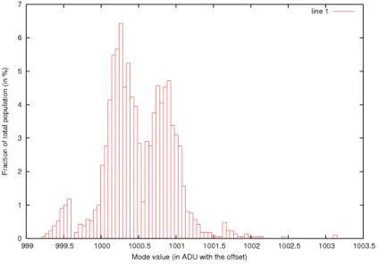
3.5.2 Overview . . . 46 3.6 Conclusion . . . 49 4 Pre-calibration 53 4.1 Introduction . . . 53 4.2 Motivation . . . 54 4.2.1 Effects . . . 54 4.2.2 Policy . . . 54 4.3 Algorithms . . . 55 4.3.1 Linear transform . . . 55 4.3.2 Dead samples . . . 57 4.4 Architecture . . . 59 4.4.1 Processing flow . . . 59 4.4.2 Sample replacement . . . 60 4.5 Conclusion . . . 60 5 Background estimation 61 5.1 Introduction . . . 61 5.1.1 Need . . . 61 5.1.2 Contributors . . . 62 5.2 Background statistic . . . 63 5.2.1 Regional background . . . 63 5.2.2 Estimator . . . 64 5.2.3 Replacement strategy . . . 66 5.2.4 Background map . . . 68 5.3 Performances . . . 69 5.3.1 Precision . . . 70 5.3.2 Robustness . . . 70 5.3.3 Representativity . . . 71 5.4 Algorithms . . . 72 5.4.1 Histograms . . . 72 5.4.2 Mode determination . . . 73 5.4.3 Interpolation . . . 75 5.5 Conclusion . . . 76

6 Simple object model 77 6.1 Introduction . . . 77 6.2 SOM . . . 77 6.3 Sample selection . . . 78 6.4 Connected-component labelling . . . 79 6.4.1 Introduction . . . 79 6.4.2 Definitions . . . 79 6.4.3 Principle . . . 80 6.4.4 Relabelling . . . 81 6.4.5 Algorithm . . . 82 6.5 SOM Descriptors . . . 87 6.6 Object queues . . . 87 6.7 Conclusion . . . 88

CONTENTS v

7 Fine object model 89

7.1 Introduction . . . 89 7.1.1 Structure . . . 89 7.2 Undesirable detections . . . 91 7.2.1 Faint objects . . . 91 7.2.2 PPEs . . . 93 7.3 Component segmentation . . . 95 7.3.1 Motivation . . . 95 7.3.2 Segmentation paradigm . . . 96 7.3.3 Markers . . . 98 7.3.4 Results . . . 102 7.4 Measurements . . . 105 7.4.1 FOM descriptors . . . 105 7.4.2 Performances . . . 107 7.5 Conclusion . . . 109

III

Implementation

111

8 Platform 113 8.1 Introduction . . . 113 8.2 Candidate platforms . . . 114 8.2.1 Digital devices . . . 114 8.2.2 Programmable hardware . . . 114 8.3 Design methodology . . . 116 8.4 Test platform . . . 120 8.4.1 Platform . . . 121 8.4.2 Programming . . . 121 8.5 Conclusion . . . 122

9 Internal architecture of the FPGA 123 9.1 Introduction . . . 123 9.2 Architecture . . . 124 9.2.1 Simplified architecture . . . 124 9.2.2 External SRAMs . . . 125 9.2.3 Clock generation . . . 125 9.2.4 Components . . . 129 9.2.5 Initialisation . . . 131 9.3 Interfaces . . . 132 9.3.1 Input interface . . . 132 9.3.2 Output interface . . . 132 9.3.3 Memory interfaces . . . 133 9.3.4 Handshake protocol . . . 135 9.4 Reset policy . . . 140 9.4.1 Introduction . . . 140 9.4.2 Implementation . . . 141 9.5 Clocks . . . 142 9.5.1 Functional . . . 142 9.5.2 Implementation . . . 143 9.5.3 Clock domains . . . 144

9.6 Design for test . . . 145

9.6.1 Debugging . . . 145

9.6.2 Conditional instantiation . . . 146

9.6.3 Initialisation sequence . . . 146

vi CONTENTS

10 Asynchronous SRAM controller 149

10.1 Introduction . . . 149 10.2 Specifications . . . 150 10.3 Design . . . 151 10.3.1 Discussion . . . 151 10.3.2 Interface . . . 154 10.3.3 General considerations . . . 154 10.4 Structure . . . 155 10.4.1 Scheduler . . . 155 10.4.2 Buffer FSM . . . 156 10.4.3 Read FSM . . . 157 10.4.4 Write FSM . . . 158 10.4.5 Fetch processes . . . 158 10.5 Implementation . . . 159 10.5.1 Performances . . . 159 10.6 SRAM VHDL model . . . 160 10.7 Conclusion . . . 163 11 Fixed-point formulae 165 11.1 Introduction . . . 165 11.2 Fixed-point arithmetics . . . 166 11.2.1 Methods . . . 166 11.2.2 Calculation error . . . 168 11.3 Modules . . . 170 11.3.1 Pre-calibration . . . 171 11.3.2 Mode determination . . . 176 11.3.3 Background interpolation . . . 182 11.3.4 Sample-wise SNR . . . 184 11.3.5 Background flux . . . 186

11.3.6 Mean background flux . . . 187

11.3.7 Object-wise SNR . . . 188 11.3.8 Barycentre . . . 189 11.4 Conclusion . . . 190 12 Processing pipeline 191 12.1 Introduction . . . 191 12.2 Design considerations . . . 192 12.2.1 Introduction . . . 192 12.2.2 Constraints . . . 193 12.2.3 Pipeline . . . 193 12.2.4 Scheduling . . . 195 12.2.5 RAM . . . 196 12.3 Components . . . 197 12.3.1 Scheduler . . . 197 12.3.2 Pre-calibration . . . 200 12.3.3 Buffering . . . 204 12.3.4 Histogram . . . 206 12.3.5 Mode . . . 213 12.3.6 Pixsel . . . 218 12.4 Conclusion . . . 221

13 Synthesis & Co. 223 13.1 Introduction . . . 223 13.2 Verification . . . 223 13.3 Synthesis . . . 224 13.3.1 Introduction . . . 224 13.3.2 Constraints . . . 225 13.3.3 Area . . . 225 13.3.4 Timing . . . 225 13.4 Conclusion . . . 227

CONTENTS vii

Conclusion

231

Appendices

235

A Test platform and setup 235

B Parameters 247

C Simulations 249

Acronyms

AA Available Addresses AC ACross scan

ACI Action Concert´ee Incitative ACP ASIC and FPGA Control Plan ADC Analog to Digital Conversion ADP ASIC and FPGA Development Plan ADU Analog Digital Unit

AF Astrometric Field AF1 First AF CCD

AGIS Astrometric Global Iterative Solution AL ALong scan

ALMA Atacama Large Millimeter Array AOCS Attitude and Orbit Control System API Application Programming Interface APM Automatic Plate Measuring AR Acceptance Review

ARS ASIC and FPGA Requirement Specification ASIC Application Specific Integrated Circuit BB Bounding Box

BER Bit-Error Rate BP Blue Photometer CC Connected-Component CCC Clock Conditioning Circuit CCD Charge-Coupled Device

CDMU Command and Data Management Unit CDR Critical Design Review

CE Chip Enable

CECC CENELEC electronic components committee

CENELEC Comit´e Europ´een de Normalisation

Electrotechnique

CI Charge Injection

CISC Complex Instruction Set Computer CL Continued Labels

CLK CLocK

CNES Centre National d’ ´Etudes Spatiales COTS Commercial-Off-The-Shelf

CPLD Complex Programmable Logic Device CPU Central Processing Unit

CS Chip Select

CTI Charge Transfer Inefficiency

CTU Central Terminal Unit (master on the OBDH bus) CU Coordination Unit

DCLK Data CLocK

DDR Detailed Design Review DFT Design For Test

DI Data In (from the PC’s standpoint) DMS Double and Multiple Star

DO Data Out (from the PC’s standpoint) DPAC Data Processing and Analysis Consortium DPAS Dual Port Asynchronous SRAM

DPU Digital Processing Unit

DPSS Dual Port Synchronous SRAM DRAM Dynamic RAM

DSNU Dark Signal Non Uniformity DU Development Unit

E Integer part of (by truncation)

ECSS European Cooperation for Space Standardisation EDA Electronic Design Automation

EDAC Error Detection And Correction EEPROM Electrically Erasable Programmable

x CONTENTS

EPROM Erasable Programmable Read-Only Memory ESA European Space Agency

ESCC European Space Component Coordination ESD ElectroStatic Discharge

ESOC European Space Operation Center FAME Full-sky Astrometric Mapping Explorer

FAST Five-hundred-meter Aperture Spherical Telescope FDIR Fault Detection, Isolation and Recovery

FET Field Effect Transistor FIFO First In First Out queue FL Freed Labels

FM Flight Model FOM Fine Object Model FOV Field Of View FPA Focal Plane Assembly

FPASS Focal Plane Assembly Static Simulator FPGA Field Programmable Gate Array FPU Floating Point Unit

FRA Feasibility and Risk Analysis report FSM Finite State Machine

FWC Full Well Capacity GD Gaia Detect (part of Pyxis)

GEPI Galaxie, ´Etoile, Physique et Instrumentation laboratory (division of OBSPM, UMR 8111) Gibis Gaia image and basic instrument simulator GNU GNU’s Not Unix

GPL General Public License

GSFC Goddard Space Flight Center specification (NASA)

GW Global Write

HiPParCoS High Precision Parallax Collecting Satellite HQ Hierarchical Queue

IAU International Astronomical Union ID IDentifier

IDE Integrated Design Environment

IEEE Institute of Electrical and Electronics Engineers

IM Inter-Module data structure IO Input/Output

ITAR International Traffic in Arms Regulations ITT Invitation To Tender

ITU Intelligent Terminal Unit (RTU with decentralised processing capabilities)

JASMINE Japan Astrometry Satellite Mission for INfrared Exploration

JTAG Joint Test Action Group (usual name used for the IEEE 1149.1 standard entitled Standard Test Access Port)

LA Label Addresses

LaMI Laboratoire de M´ethodes Informatiques (UMR

8042)

LET Linear Energy Transfer LSB Least Significant Bit LSF Line-Spread Function LUT Look-Up Table LV Label Values

MIPS Million Instructions Per Second MoM Minutes of Meeting

MOS Metal-Oxide-Semiconductor MRD Mission Requirement Document MSB Most Significant Bit

MTF Modulation Transfer Function

NASA National Aeronautics and Space Administration NIEL Non-Ionizing Energy Loss

NGST Next Generation Space Telescope OBDH On-Board Data Handling OBSPM OBServatoire de Paris Meudon OF Object Feature

OLMC Output Logic Macro Cell OS Operating Software

PC Personal Computer PCB Printed Circuit Board

PCDU Power Control and Distribution Unit PDF Probability Density Function

CONTENTS xi

PDHS Payload Data Handling Subsystem PDH-S Payload Data Handling Support contract PDHU Payload Data Handling Unit (supervisor) PDR Preliminary Design Review

PEM Proximity Electronic Module PIA Programmable Interconnect Array PLD Programmable Logic Device PLL Phase-Locked Loop

PLM PayLoad Module PPE Prompt Particle Event

PPN Parameterized Post-Newtonian

PRiSM Parall´elisme R´eseaux Syst`emes Mod´elisation (UMR 8144)

PSF Point-Spread Function

PRNU Pixel Response Non Uniformity PSRAM Pseudo-Static RAM

QA Quality Assurance

QML Qualified Manufacturing Line QPL Qualified Part List

QR Qualification Review RAM Random Access Memory

RISC Reduced Instruction Set Computer RM Relabeling Map

RMS Root Mean Square ROM Read-Only Memory RON Read-Out Noise RP Red Photometer

RPM Relabelling Paths Memory RTL Register Transfer Level

RTU Remote Terminal Unit (slave on the OBDH bus) RVS Radial Velocity Spectrometer

SCL Static Chained List SCLK Sram CLocK SEL Single Event Latch-up SET Single Event Transient SEU Single Event Upset

SKA Square Kilometer Array SM Sky Mapper

SMP Symmetric MultiProcessing SNR Signal to Noise Ratio SOM Simple Object Model

SPARC Scalable Processor Architecture SPAS Single Port Asynchronous SRAM SPC Science Programme Committee (ESA) SPSS Single Port Synchronous SRAM SRAM Static RAM

SREM Standard Radiation Environment Monitor SRR System Requirement Review

SSMM Solid State Mass Memory SSO Simultaneous Switching Outputs SVM SerVice Module

SWA Sliding Window Algorithm SWG Simulation Working Group TBC To Be Confirmed

TBD To Be Defined TC TeleCommand

TDA Technical Definition Assistance TDI Time-Delay Integration

TID Total Ionizing Dose TM TeleMetry

TMR Triple Module Redundancy TTL Transistor-Transitor Level

TTVS Techniques et Technologies des V´ehicules

Spatiaux (a course on spaceborne technology organised by CNES)

URD User Requirement Document

VERA VLBI Exploration of Radio Astronomy VHDL VHSIC Hardware Description Language VHSIC Very High Speed Integrated Circuits VLBA Very Long Baseline Array

VPU Video Processing Unit WD Window Data

xii CONTENTS

WED White Electronics Designs WFE WaveFront Error

XNOR Negated eXclusive OR XOR eXclusive OR

Foreword

This thesis presents an analysis of the problem of detecting objects of interest on board ESA’s cornerstone mission Gaia. Based on an understanding of the scientific context, an algorithmic formulation is proposed which is compatible with operation in space while being coherent with the use intended for the data. To further ascertain this conclusion, steps are taken for the elaboration of a hardware demonstrator as part of the mixed architecture which is envisaged. This offers an opportunity to evaluate performances altogether scientifically and technically and conclude on the R&D effort.

The work summarised in these pages originates in the phase A studies carried out by the OBDH working group to assess achievable performance and assist in the production of specifications. As such it is deeply rooted in the preparation of the Gaia mission. As a consequence, the role it has assumed in this frame, while considerably enriching our reflection, has also imposed restraints on our search for solutions. To increase the probability of success within the project’s time line, previously successful approaches were selected as starting point and have led, because of the imperatives of consistency in our collaborations, in algorithms which are not wholly original in themselves. Neverthe-less, we believe that their expressions in the system devised, the end-to-end view to the question addressed and the solutions and trade-offs upon which the technical realisation builds remain worthy of interest, especially considering how Gaia’s processing requirements are orders of magnitude above other existing or planned systems.

Conversely, the underlying engineering has been of relevance to the project in return and is an endeavour to contribute to the field of space technology, however modestly. During phase A, beside providing grounds for establishing scientific requirements, the full data acquisition model built by the OBDH working group (Pyxis) was placed at the heart of the PDHE TDA study (2004-2005) to dimension the on-board electronics and collaboration with the contractor was made official by the PDH-S contract between OBSPM and ESA (2004-2005). When the industrial phases began, this contract was prolonged (2005-2007) to support the prime contractor with some of the expertise gathered and explanations on the need, algorithmic discussions and document and specification reviews have been corollaries of our developments. In parallel, the design of the demonstrator has been conducted within the ALGOL ACI (2004-2007) which, with computer scientists (PRiSM and LaMI), has sought to reconcile the masses of data generated on board satellites with the telemetry limitations in a more general sense. Accordingly, the results collected in this volume are not the result of individual isolated work but proceed from all these different frames. Tab. 1 recalls the contributions of my collaborators, may they be wholeheartedly thanked for them.

In March 2006, the design of the on-board processing subsystem became the responsibility of the prime contractor for Gaia (EADS Astrium SAS). As a consequence, Pyxis, and the detection scheme described in this text in particular, are only considered as reference work since then. Although comparison with the industrial application would be highly enlightening, it is proprietary information covered by a non-disclosure agreement so that the corresponding strategies are not further mentioned in this document.

After a first part introducing the concept and needs of Gaia (chapter 1), then the constraints applicable to on-board processing (chapter 2), the second focuses on the algorithms proper (chapter 3). To this end, approaches to the calibration of the CCD data (chapter 4), the background estimation (chapter 5) and finally the identification (chapter 6) and the measurement of objects (chapter 7) are discussed in the light of the specifications. High level descriptions are given in this part corresponding to the development of a software prototype (GD part of Pyxis) partly intended to evaluate functional performance and partly useful as a reference model. Finally, a third part refines the sample-based operations in the process of porting them to a test platform equipped with an FPGA. After presenting the technology and methodology for hardware implantation (chapter 8), an architecture is selected which facilitates testing (chapter 9) and provides facilities to the processing module, notably in terms of access to external memory (chapter 10). After translating floating-point formulae to fixed-point equivalents for compatibility with the hardware (chapter 11), the core calculations can then be derived from part II (chapter 12) before an overall inspection of the demonstrator is carried out in a concluding chapter (chapter 13). Chapters 10 and 12 are notably technical because of the intricacies of hardware implementation and are hence easier to follow for those familiar with electronics.

xiv Foreword

Contributions

3 Introduction S. Mignot, F. Ch´ereau, based on APM [1] & [2] and Sextractor [3]

4 Pre-calibration S. Mignot, P. Laporte

5 Background S. Mignot, F. Arenou, with interpolation based on [4] by F. Patat

7 Fine object model S. Mignot, based on the watershed transform by F. Meyer [5] and by J.C. Klein [6]

8 Platform S. Mignot, F. Rigaud, G. Fasola

11 Fixed-point S. Mignot, F. Arenou

12 Pipeline S. Mignot, P. Laporte

A Platform F. Rigaud, G. Fasola, S. Mignot

C Simulations F. Ch´ereau, C. Babusiaux

PDH-S

Management S. Mignot

Team S. Mignot, F. Ch´ereau, C. Macabiau, F. Arenou, C. Babusiaux

Pyxis

Integration F. Ch´ereau, S. Mignot, F. Arenou

Validation F. Arenou, S. Mignot

Pre-calibration S. Mignot

Detection S. Mignot, F. Ch´ereau

Propagation F. Ch´ereau

Selection J. Chaussard, F. Ch´ereau, F. Arenou

Confirmation S. Mignot

Assembly S. Mignot, F. Ch´ereau

Sensitivity C. Macabiau

Simulations F. Arenou, F. Ch´ereau, S. Mignot

ALGOL ACI

Laboratories PRiSM, GEPI, LaMI,

GEPI team S. Mignot, P. Laporte, F. Arenou, F. Rigaud

Part I

Chapter 1

The Gaia mission

Contents

1.1 Introduction . . . 3 1.2 Scientific return . . . 5 1.3 The satellite . . . 7 1.3.1 Measurement principle . . . 7 1.3.2 Overview of operation . . . 9 1.3.3 CCD technology . . . 13 1.4 Conclusion . . . 17

1.1

Introduction

Concept

The GAIA mission was first proposed in response to a call for ideas for ESA’s next cornerstone missions (Horizon 2000+ program) in 1993 by Lindegren et al. [7] [8] to build on the success of HiPParCoS [9]. Beside achieving sub-milliarcsecond (mas) astrometry1 _{in visible light, the latter’s intent was extended to perform a survey of the Galaxy}

to tackle questions relative to its origin, structure and evolution. To this end, following the principle established by HiPParCoS, a largely over-determined set of high precision observations is to be collected from two distant FOVs2 _at

different epochs to not only allow the determination of the astrometric parameters but also, simultaneously, permit the calibration of the instrument. Photometric and spectroscopic data are to be collected jointly to enrich the resulting phase-space map of the Galaxy with astrophysical information in a manner resembling the Tycho catalogue3_{. With}

a sample amounting to approximately 1% of the Galaxy4_{, of the order of one billion objects are observed on average}

during 80 transits and in 12 to 15 CCDs each time. As one may easily imagine, this wealth of data, with its volume and diversity, proposes scientific and technical challenges to both the ground and the space segments.

This latter aspect is made all the more critical by the decision to place Gaia on a small amplitude Lissajous5 orbit around L2, the second co-linear libration point in the Earth-Sun system about 1.5 × 106 km away from the

Earth6 _{(Fig. 1.1). Communications over such distances are more difficult due to the propagation delay and the}

attenuation. Besides implying that the spacecraft and the payload must be highly autonomous, this significantly reduces the available bandwidth for transmissions to ground, as compared to geostationary orbits for instance. With the intermittent visibility from ground due to the cost of operating antennas (currently two, respectively in Spain (Cebreros) and Australia (New Norcia)), it is obvious that HiPParCoS’s strategy of piping data to ground directly

1_{Astrometry is the discipline in astronomy concerned with measuring positions and motions. Positions are classically determined as two}

angles on the celestial sphere of reference (right ascension and declination) complemented by the parallax. The parallax corresponds to the angular extension of the semi-major axis of the Earth’s revolution around the Sun, which knowing the Earth’s orbit and the direction of the star, provides a measure of distance expressed in parsec. One parsec is the distance at which this semi-major axis represents one arcsecond (as), ie. 2.78 × 10−4degrees and corresponds to 3.262 light years (3.086 × 1013_km).

2_{ie. separated by a large angle on the sphere (106, 5 deg).}

3_{An auxiliary star mapper on board HiPParCoS was used to produce a second catalogue, the “Tycho catalogue”, with reduced astrometric}

precision but with photometry.

4_{The 1% figure is the one advertised by [10] but the total visible mass is likely above 10}9_{solar masses with stars less massive than the}

Sun in average.

5_{Lissajous curves, of the general form (x = a.sin(nt + c), y = b.sin(t)), describe harmonic motions resulting from the combination of}

several harmonic oscillators and can be periodic or quasi-periodic.

4 The Gaia mission

after acquisition is not realistic for Gaia. Instead, the constraints call for sophisticated processing and storage on board to first reduce the volume then manage the flow through the downlink facility.

Figure 1.1: The Sun, the Earth and Gaia’s Lissajous orbit in the reference system co-rotating with the Earth around the Sun (courtesy of ESA [10], scales are not respected).

A bit of history. . .

The first satellite concept which emerged relied on interferometry as a natural means of improving the precision of individual measurements [12] [13]. Interestingly enough, the “Concept and Technology Study”, begun in July 1997, examined the corresponding constraints in terms of pixel size, alignment of mirrors, photon counts and resulting data rate and found that the astrometric accuracy could be improved, completeness obtained at a fainter limit and the overall design simplified by merging the two halves of each primary mirror. Hence, the interferometric option was discarded and the preference given to a “better, cheaper, faster” direct imaging system [10]. After this founding principle was adopted7_{several successive configurations were envisaged for the payload: [10] proposed three telescopes}8

and two focal planes mounted on a hexagonal optical bench. Overall size reduction was later carried out (2002) to fit the satellite within the Soyouz-Fregat fairing in a global cost reduction endeavour. Finally, in response to ESA’s ITT, EADS Astrium SAS’s9 _{proposal was accepted in 2006 featuring only two telescopes and a single focal plane for}

further reduction of the complexity of the payload.

This series of designs has largely affected the payload and the imaging properties but the key elements of on-board operation have remained applicable throughout. From a high level point of view, these are relevant to commanding the acquisition of snapshots around the objects of interest, managing the resulting data on board before it can be transmitted to ground and providing estimates for the attitude control loop based on the apparent motion of objects. As a consequence, detecting the objects is of critical importance not only for the quality of the scientific return of the mission but also, quite simply, for nominal operation of the instruments.

Schedule

Fig. 1.2 illustrates ESA’s schedule for Gaia. The project is currently in phase B2, generally denominated “preliminary definition” in ECSS standards, but referred to as “detailed design” for Gaia, and negotiations for the transition to phase C are on-going between Astrium and ESA. With a recommendation for being no later than 2012 by the SPC, launch is planned for December 2011 from Kourou in French Guiana with a Soyouz-Fregat launcher. After six months of transit to L2, the satellite would remain in nominal operation for 5 year (+1 extended time) with an estimated 10% system, satellite or ground segment dead time. Accordingly, accounting for some margin for the determination of parameters depending on the complete data set, the overall refinements and verifications, the final catalogue is expected to be published around 2020. Considering that HiPParCoS’s results, for 118 218 stars, fill 16 volumes, R&D will be also be necessary for the former’s format and distribution. . .

7_{The GAIA acronym for “Global Astrometric Interferometer for Astrophysics”, then became simply a name “Gaia” as will be spelled}

hereafter.

8_{Two for the astrometric measurements and one for the medium band photometric and spectroscopic ones.} 9_{Hereafter Astrium.}

1.2 Scientific return 5

Figure 1.2: Gaia’s official schedule (courtesy of ESA (website)).

1.2

Scientific return

Although only a “small” percent of the Galaxy, Gaia’s sample will be of remarkable relevance to many fields of astronomy and astrophysics thanks to its high precision, bulk (20 Terabytes of compressed raw science data with a database exceeding the petabyte) and completeness. Beside the main aims of the mission emphasising astrometry and stellar populations, many by-products can be derived by data mining in the Gaia catalogue as Tab. 1.1 illustrates.

A crucial aspect of the catalogue for epoch-dependent studies and for statistical inference is Gaia’s selection function. The MRD [14] has three specifications constraining object selection on a transit basis:

Specification 1 (SCI-220) More than 95% per FOV of the transits of single objects and multiple systems over the magnitude10 _{range specified in SCI-200 and SCI-210 shall be observed. Missing transits shall be accounted for in the}

overall error budget.

Specification 2 (SCI-200) The bright object completeness limit shall be not fainter than11: • V = 6.0 for unreddened B1V stars,

• V = 6.2 for unreddened G2V stars, and • V = 8.4 for unreddened M6V stars.

Specification 3 (SCI-210) The faint object completeness limit shall be not brighter than: • V = 20.0 for unreddened B1V stars,

• V = 20.2 for unreddened G2V stars, and • V = 22.4 for unreddened M6V stars.

While predictable causes of heterogeneity12_{can be accounted for, those related to failed detection for instance are}

more problematic. Although complex due to the size of the database, random effects can be identified with the help of cross-transit matching. On the contrary, systematic ones will distort the resulting picture of the Galaxy. Meeting all the expectations listed in Tab. 1.1 then calls for a detection mechanism both highly reliable and sufficiently versatile to accommodate the variety of observing conditions for the entire spectrum of objects of interest.

10_{Magnitude relates to flux according to m = −2.5log(}f

f0) = m0− 2.5log(f ) and hence decreases when the flux increases.

11_{V designates the magnitude measured in one of the three bands of the standardised Johnson-Morgan photometric system. It is often}

termed the “visual” magnitude because this band is in the visible domain. B1V, G2V etc. designate stellar classes in the Harvard spectral classification and correspond essentially to different colours of main sequence stars as a result of different effective surface temperatures which are connected to the astrophysical nature of the stars (mass & radius mainly).

12_{For instance fluctuations in photometric or radial velocity precision due to the fact that not all detected objects are imaged in the}

6 The Gaia mission

Domain Contribution Description

Structure of the Galaxy Positions and kinematics for stars in all populations and struc-tures (thin disk, thick disk, halo, bulge, spiral arms, bar, glob-ular clusters, star-forming regions etc.).

Galactic physics Age and metallicity For the characterisation of populations together with the

de-tection of remarkably metal-poor/rich or old objects.

Tracers of evolution Tidally-disrupted accretion debris.

Dark matter

Unresolved galaxies Photometry for more than 106.

Extra-galactic physics Local Group Dynamics and parallaxes (direct measurements for the

bright-est objects).

Stellar types Populations at the different stages of evolution (including

pre-main sequence and rapid evolutionary phases), Hertzprung-Russel diagram.

Stellar physics Astrophysical parameters Mass, radius, luminosity, temperature, chemical composition

for the brightest stars.

Binary stars 107 resolved binaries expected within 250 pc.

Variable stars 1.8 × 107 expected.

Distances In the Galaxy and the Local Group.

Distances Quasars 5 × 105_{expected for the construction of a reference system.}

& Reference systems Cepheids & RR Lyrae Several 103_{& 7.4 × 10}4_{expected for recalibrating the “distance}

ladder” in the Universe.

Asteroids 5 × 105expected (from the Main Belt essentially but also

Tro-jan, trans-Neptunian & Plutinos) with masses and rotation for part of them.

Solar system Near-earth objects 105 _expected.

Orbits Improvement by a factor 30.

Sun Improvement on the measurement of the solar quadrupole

mo-ment J2.

Exotic objects

Burst sources

Extra-solar planets 3 × 104 expected with Jupiter-like masses up to 200 pc, some

with orbits, some only based on transits. Brown & white dwarves Several 104 _expected.

Supernovae 105 _expected.

Micro-lensing

General relativity Assess need for scalar correction, high precision PPN γ and β

parameters.

Fundamental physics Gravitational waves Energy determination over a certain frequency range.

Variability of constants Rate of change of G.

1.3 The satellite 7

1.3

The satellite

1.3.1

Measurement principle

Scanning law

Gaia’s measurement principle is analogous to HiPParCoS’s except in respect to technology, to orbit and to the intro-duction of spectro-photometry and a RVS complementing the five-dimensional astrometric parameters into a complete phase-space map. Although relying on a pre-selected list of 118 218 stars, pointed operation was made possible, a scan-ning strategy could be devised for HiPParCoS thanks to the distribution of targets over the celestial sphere imposed by the purpose of building a reference system. With Gaia’s homogeneous survey objective, this argument applies twofold, with the corresponding benefits of reduced needs in terms of propellant and higher precision attitude reconstruction. As a consequence, Gaia’s observing principle could reduce to: “measure everything transiting across the detectors”. Technical considerations make this undesirable however, as discussed below, so the concept should rather be restated as: “measure everything in the magnitude range of interest transiting across the detectors”. It is worth stressing that this restriction simply corresponds to acknowledging that precision is fundamentally limited by the photon statistics and that it remains fully in line with Gaia’s completeness aims provided a sufficient number of photons are received for all objects of interest. Nevertheless, the scanning concept combined with the magnitude-driven object selection have far-reaching consequences concerning the design of the spacecraft and the payload.

Gaia’s motion corresponds to a free-fall of its centre of gravity on the selected quasi-periodic Lissajous orbit13 (Fig. 1.3) combined with spin and precession movements of the spacecraft around it (Fig. 1.4). The corresponding rates, along with the initial conditions resulting from the injection on the orbit, impact on the coverage of the sphere, particularly as regards homogeneity and the frequency of great circles14 _{running parallel to the galactic plane or}

crossing the galactic centre. With stellar densities fluctuating between an average 25 000 stars/deg2 over the entire sky, a typical 150 000 stars/deg2 in the disk and a maximum of 3 000 000 stars/deg2 in the low extinction zones of the galactic centre (Baade’s windows), these events are of special relevance for on-board operation, be it processing or data storage. Besides, one of the properties of the coverages obtained is that the variable number of observations for stars at different galactic coordinates (80 transits on average) tends to be unfavourable to dense areas. As one may guess, this is rather fortunate as far as dimensioning the processing resources is concerned. It is, however, problematic scientifically speaking because these areas suffer from increased crowding: the ratio between the number of parameters to be estimated and the volume of data collected increases because multiple objects fall in the same window, thereby affecting the final precision. Hence, stringent reliability expectations result on the on-board processing for such configurations in spite of their being intrinsically more difficult to handle.

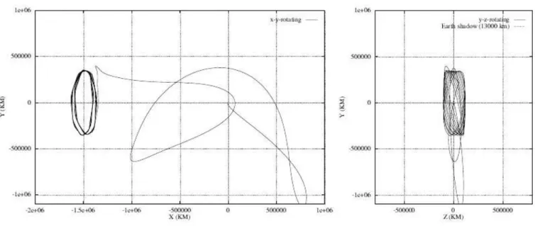
Figure 1.3: A typical one-manoeuvre transfer and Lissajous orbit for Gaia with a launch on 9/04/2009 as seen from two different viewpoints (courtesy of M. Hechler et al. [15])

13_{With maintenance manoeuvres expected about once per month to counteract the instability [15].} 14_{A “great circle” denotes the trace of the FOVs during one spin period.}

8 The Gaia mission

Figure 1.4: Parameters of Gaia’s attitude (spin rate: 60 arcsec/s, period: 6h) and scanning law (courtesy of DPAC, [16])

Astrometry

Just like HiPParCoS, Gaia’s astrometric measurements are performed in two well separated FOVs and only one-dimensionally. The former relates to the desire to obtain absolute positioning of the objects as opposed to a relative one. With the two FOVs, each object is referenced against all those of the other field, instead of only versus the neighbouring ones. The corresponding large scale constraints translate into a form of “rigidity” in the set of measurements, as opposed to summing small distortions when integrating between one line of sight and the next. Technically speaking, it implies that two FOVs must be observed in comparable conditions at all times, thus doubling the load on average.

Collecting one-dimensional data corresponds to measuring only the objects’ longitude (abscissa) on the great circles. It yields precision improvements on individual measurements due to a higher SNR and the determination of fewer parameters based on a given data set. Design-wise, although the entire payload can hardly be simplified to the extent of working with only one dimension because of the need to estimate two rates for attitude control (for spin and precession with a precision of the order of the mas/s), it nevertheless leads to significant simplifications as regards the volume of scientific data per observation and the different angular resolution and stability constraints in the two directions. Conversely, the degraded information calls for collecting more data since two “missing” dimensions need to be inferred from the data set during the analysis. This is possible by globally fitting the stellar motion model to the set of abscissa on the great circles acquired during the entire mission, provided objects can be identified by inter-transit cross-matching. Fig. 1.5 illustrates how the parallax and proper motion can be jointly estimated in this process.

While the astrometric data acquired on a long time base are valuable for the determination of the parallax and proper motion, shorter term ones are relevant, for example, to the study of binary systems. As Fig. 1.5 illustrates, the presence of a companion object perturbs the motion of the primary object around the system’s centre of gravity which may only be characterised if the angular and temporal resolutions are sufficiently high.

Photometry and spectroscopy

Like the astrometric data above, “instantaneous” photometry and spectroscopy are relevant for the brighter objects since they provide valuable multi-epoch data for studies related to variability. Conversely, fainter ones are affected by the degradation of the photon statistics which results from dispersing the light and require combining measurements to increase the SNR before any interpretation can become possible. With the intent to cover a large spectrum of astrophysical investigations, spectro-photometry is carried out instead of relying on distinct multiple photometric bands and a moderate resolution was selected for the RVS (λ/∆λ = 11500). With Astrium’s decision to rely on a single focal plane, acquisition of this data follows from collecting the astrometric one (Fig. 1.8) so that, from an on-board operation point of view, it calls for a limited amount of additional processing, while the data represents the most significant contribution to the problem of data management (storage and telemetry).

1.3 The satellite 9

Figure 1.5: Principle of the determination of the parallax and proper motion of stars (courtesy of ESA, [10]). The apparent motion is the result of the projection on the celestial sphere of the composition of the star’s motion in the Galaxy (proper motion) with the reflex motion induced by the revolution of the Earth-satellite system around the Sun (parallax). The proper motion may be coarsely estimated by linear regression, while the parallax corresponds to the semi-major axis of the ellipse recovered after compensation of the proper motion (although in practice all parameters are estimated jointly). Additionally on this figure, the perturbation resulting from the presence of an undetected companion object is illustrated by the difference between the plain and the dotted lines (isolated star model).

Data reduction

Fig. 1.6 illustrates the dependencies existing between the various types of data acquired and the diversity of products to be extracted through the different analyses. Although complex, this representation is highly simplified compared to the intrinsically convoluted problem of disentangling the multiplicity of scientific and instrumental effects.

Beside the need for numerous observations, attribution of data to physical entities (“Object matching” in Fig. 1.6) relies on the capability to compare several transits and cross-match observations. This is only possible if preliminary attitude predictions are available between each of the observing instants to determine the directions of the two lines of sight while, conversely, attitude reconstruction itself relies on the identification of the contents of the FOVs. To solve this problem in spite of the coupling between the two, a global iterative procedure (AGIS) should jointly esti-mate attitude, calibration and astrometric parameters for a subset of well-behaved stars. It is worth noting that its convergence depends crucially on the quality of the data received from the satellite and on the reliability of on-board detection in particular because of the need to predict observations rapidly after a first round of great circles covering the celestial sphere.

1.3.2

Overview of operation

Orbit

As for HiPParCoS, the decision to make Gaia a space mission results from the large time base required for astrometry. The very definition of the parallax implies that several measurements from significantly different positions of the Earth on its orbit around the Sun are necessary. Similarly, proper motion estimates, as first order models of the projection of the displacement of stars on the sphere, call for multiple points with large separations in time. In both cases, the quantity of interest is intrinsically of relative nature which calls for ensuring that data are comparable in spite of their belonging to different epochs. On ground, calibration issues resulting from short term variability of the instrument parameters – mainly due to thermal and gravity deformation – introduce systematic effects which limit the achievable precision in a manner incompatible with seeking parallaxes, at least based on existing technology. Conversely, in space, the absence of atmosphere and of gravity together with the possibility to achieve highly precise thermal control

10 The Gaia mission

Figure 1.6: Overview of the data reduction processes for the interpretation of Gaia’s data (with acquired data in red, models and products in black and processes in purple). This figure corresponds to the 2002 baseline design in which separate broad and medium band photometers where planned. These have been replaced by the BP and RP spectro-photometers (section 1.3.2). Courtesy of M. A. C. Perryman.

of the payload provide more favourable circumstances for high precision, systematic and homogeneous measurements collected with a single well-calibrated instrument.

Although HiPParCoS, intended to be geostationary, did operate successfully from a highly elliptical orbit between 507 and 35 888 km, orbit is a key design driver. From a technical point of view, it impacts on mass mainly, as a consequence of the propellant budget for manoeuvres during transfer and for attitude and orbit control. Mass, in turn, impacts on the selection of the launcher which places constraints on cost and volume. . . Tab. 1.2 recalls the main elements in the trade-off performed between possible orbits for Gaia. This table lacks an indication of weights attributed to the criteria, but following the argument above, the decisive concern has been to favour stability. Lissajous orbits around L2 offer a very stable thermal environment (for the payload), means of altogether avoiding eclipses (for the power subsystem), the absence of Earth or Moon occultations (for observations) and reduced dynamical perturbations (for pointing accuracy and maintenance).

As already mentioned, the principal downside to this option is communication with ground because of partial visibility from a single station and reduced transmission rates whatever the transmitter and antenna technology used. This calls for autonomous operation and large and intelligent data management and storage on board. These are the main requirements applicable to the on-board computing. It is worth noting that while the geostationary alternative, considered feasible in [10]15_{, would induce simplifications as regards the general data management, the need for}

on-board detection and object characterisation would remain nevertheless. Spacecraft and the payload

The Gaia satellite is built upon a custom platform. As illustrated Fig. 1.7a, the satellite is segmented in two parts. Away from the Sun, the thermal tent houses a hexagonal optical bench (3 m in diameter) supporting the telescopes corresponding to the two FOVs, the 9 mirrors used to fold the two 35 m focal lengths, the dispersive optics for the spectro-photometers, the RVS and the FPA. This part of the satellite should be a region of passive thermal stability of the order of 0.1 millikelvin. Additionally, silicon carbide (SiC) material is used for the optical bench for its very

15_{Quoting: “The study showed that the main problem in geostationary orbit is the presence of eclipses (a standard feature of geostationary}

orbits). These are however not a problem in terms of thermal control if the astronomical observations are performed also during the eclipse: the main driver in the thermal control is in fact not the external solar radiation, but rather the internal power dissipated by the electronics. Thus, if sufficiently large on-board batteries are included observations can be performed into eclipse. Thus the study showed that either orbit is suitable for GAIA, if necessary.”

1.3 The satellite 11

Table 1.2: Elements of the orbit trade-off conducted by ESOC studies for Gaia as recalled in [10] (with ’-’, ’*’, ’**’ and ’***’ in increasing preference order) and leading to the selection of an orbit around L2.

low coefficient of thermal expansion. The main reason for such stringent requirements is the need to tightly monitor fluctuations on the angle between the two FOVs, the “basic angle” (106.5 deg), to obtain absolute astrometry without the need for external references for calibration.

On the other side, a service module structure, thermally insulated from the bench, contains the propellant reservoirs as well as all the equipment susceptible of variable thermal dissipation: the star trackers necessary for the acquisition of the nominal scanning law, the Li-Ion battery, the X band transponders, a particle detector SREM measuring the particle fluences, the phased-array antenna and all hardware for the processing (chapter 2). Attached to this module, a large deployable sun shield, 10 m in diameter, protects the telescopes from the Sun’s unwanted light and contributes to the thermal control. Solar panels are fixed on this shield for a power generation with high efficiency due to the constant orientation to the Sun (Fig. 1.4).

Focal plane assembly

As already mentioned and visible on Fig. 1.7c, the two FOVs are combined by the M4 and M’4 mirrors and imaged by a single focal plane. The design of the telescopes and of the focal plane is driven by the photon statistics which ultimately limits the final precision. An aperture of 1.45 × 0.5 m2 _{has been selected for the telescopes, leading to a}

focal plane extending over approximately 1.0 × 0.5 m2_{. The needs to image the data at a very high angular resolution}

(the reason for the 35 m focal length) and to have long exposures are antagonistic in the current and projected states of technology for detectors. The former indeed calls for a small pixel size and the latter implies detectors of large dimensions while state-of-the-art CCDs are “only” of the order of 4000 × 4000 pixels. As a trade-off, the focal plane is tiled with large area full-frame CCDs which yield segmented integration16_.

102 CCDs dedicated to scientific observations are organised in 7 rows17and 16 columns to form the FPA illustrated Fig. 1.8a. The rows function independently from one another to minimise data loss in case of malfunction of one of them, thereby avoiding the need for any further redundancy. Different tasks are attributed to the CCDs column-wise because the objects traverse the focal plane from left to right:

1. SM1 & SM2. These two series of CCDs image only objects from one of the FOVs18 _{(the other one being}

16_{Conversely, were it possible to image the entire focal plane with a single CCD, it would not be desirable due to AC and AL smearing}

and PPEs in spite of significant improvements in the focal plane’s complexity and reduction of the data flow.

17_{The FPA also houses an additional four used for the monitoring of the basic angle and the measurement of the wavefront errors.} 18_{Knowing from which FOV objects originate is a considerable simplification:}

• for tracking objects across the focal plane (since objects from the two FOVs have different apparent AC velocities), • for entering observations in the database and for cross-matching objects between transits,

• for unambiguously determining the attitude of the satellite at all times. .

12 The Gaia mission

Figure 1.7: The Gaia satellite as planned in phase B2 (courtesy of Astrium). Left (a): exploded view of the satellite. Top right (b): external view of the satellite with the thermal tent, the apertures of the two telescopes and the deployable sun-shield. Bottom right (c): the hexagonal optical bench supporting the two telescopes with the intermediate mirrors and the focal plane.

masked). They are entirely read-out for the purpose of detecting the objects entering the focal plane and to be subsequently observed. To increase the SNR and reduce the processing load, pixels are not read one by one but in samples: 2 pixels AL by 2 pixels AC (2 × 2).

2. AF1. The objects identified in SM1 or SM2 are confirmed in AF1 to ensure they correspond to astrophysical sources and not to noise or PPEs. Additionally, this second two-dimensional observation allows for estimating attitude parameters as part of the corresponding control loop. To make the AF1 data also relevant for on-ground astrometric exploitation, the CCD is not entirely read-out. Instead, only rectangular windows are read-out for better noise performance (section 1.3.3) based on the objects’ previously estimated locations in SM and extrapolated using the nominal attitude parameters.

3. AF2-AF9. The observations performed in AF1 are repeated between AF2 and AF9 to improve the transit’s location estimate versus photon statistics. One-dimensional data are acquired19_{in each and larger regions (in AL)}

are imaged in AF2, AF5 and AF8 for the purpose of searching the vicinity of objects of interest for companion stars fainter than V = 20 which might perturb the analysis.

4. BP & RP. Low resolution spectra are produced in BP and RP with the main intent of providing multiple band photometry with two CCDs: the first optimised towards the blue end of the visible domain (BP), the other towards the red (RP). This approach has the particular advantage of solving the problem of accommodating a series of filters without multiplying the number of CCDs and degrading optical quality20_{. Beside the astrophysical}

value of this information, measuring the chromaticity of the objects is required for full exploitation of the

19_{For bright objects, two-dimensional data is acquired in AF, BP/RP and RVS CCDs because of the need for finer calibrations.} 20_{As was the case in the baseline design of 2002, where one CCD was allocated for each band – which in turn called for a dedicated}

1.3 The satellite 13

astrometric data since the PSF depends on the objects’ colour. One-dimensional data is acquired in both, with pixels corresponding to a mixture of photometric bands depending on the sub-pixel location of the object and its apparent AL velocity compared to the TDI.

5. RVS1-RVS3. Average resolution spectra (11 500) are acquired in the RVS CCDs to estimate the velocities of the objects along the line of sight via shifts in the absorption lines (in particular the CaII lines) resulting from the Doppler effect. For objects with higher SNRs, the spectra also provide estimates of astrophysical parameters (the effective temperature, chemical composition, the surface gravity etc.).

SM1-2 AF1 - 9 BP 420 mm 0.69° RP RVS BAM BAM WFS WFS 0s 10.6 15.5 30.1 49.5 56.3 64.1 0s 5.8 10.7 25.3 44.7 51.5 59.3 sec sec FOV1 FOV2 930 mm

Figure 1.8: Organisation of Gaia’s focal plane as planned in phase B2. Left (a): focal plane assembly (courtesy of DPAC [16]). Right (b): dimensions of the individual CCDs (courtesy of A. Short et al. [17]). In spite of the orientation on this figure, Gaia terminology designates with “TDI lines” the sets of pixels parallel to the read-out register (vertically) and as columns those traversed by the charged in the course of the TDI (horizontally).

1.3.3

CCD technology

Time Delay Integration

As a result of the satellite’s spin, the stars transit across the FPA and suggest to define two directions: the along-scan (AL) one parallel to the overall movement of the objects (the abscissa in Fig. 1.8a) and the across scan (AC) one orthogonally. Conventional exposures are not possible because the stars’ movement is two dimensional: due to the precession of the spin axis and to the projection of the image sphere onto the focal plane, smearing would result in the two directions. This is incompatible with the astrometric need for very high angular resolution in at least one. Instead of “static” exposures, “dynamic” ones are carried out by operating the CCDs in a TDI mode instead. This mode shifts the charges collected in the pixels across the CCD matrix at a rate selected to exactly compensate the displacement of the objects. As the combined spin and precession movements lead to both higher and constant AL velocities versus varying AC ones, the AL axis is preferred for this to allow longer integration.

Read-out

As a consequence, the image data is not acquired as a series of snapshots to be processed individually but rather as a single continuous travelling shot stretching over the five years of the mission. It cannot, hence, be read in a single pass yielding a complete image but is, instead, read column per column21as on Fig. 1.8b, coherently with the movement of charges induced by the TDI. The read stage then “simply” consists in shifting the charges into a parallel-in serial-out register used for read-out instead of the next line of pixels.

The CCDs, as usual, comprise two-dimensional arrays of pixels. Although, one might think of collapsing the AC resolution entirely (ie. to a single pixel) to acquire data only one-dimensionally, this is not possible since objects should be observed independently as far as feasible (otherwise additional mixing parameters will need to be estimated at the

14 The Gaia mission

expense of astrometric precision). The read-out registers implanted on Gaia’s CCDs offer a simple and efficient way of reducing the AC resolution locally around each object. Intuitively, the manner in which charges are shifted into the amplifier allows for summing adjacent AC pixels. With interest in some pixels only (where the objects are) and not others, summation can be extended over entire intervals either to form larger data units or to efficiently flush the content of the register.

Structurally speaking it would be possible to also use the read-out register to merge photo-electrons from different pixels in the AL direction by shifting charges from the pixel matrix during two TDI periods22 without intermediate read-out. However, to isolate the read-out register from the pixel matrix, it is preferable to insert a summing register for this purpose23. The two combined allow of reading n × m pixels as a single one – an operation known as “binning” and producing “samples” in Gaia terminology – with the only limitation that samples belonging to the same TDI are necessarily of the same AL dimension.

The benefit of reading samples rather than pixels wherever possible stems from the fact that for electronic noise reasons, it is desirable to read the data at the slowest possible rate. This is because estimation of the photon signal is based on repeatedly measuring both the closest available reference voltage and that of the output capacitor. Slower charge transfers translate in leaving time for the electrical state of each to stabilise before new charges are ushered in and sampling occurs. For this purpose, the read-out register is clocked at two different frequencies: a faster one for flushing a majority of pixels and a slower one for transferring the pixels of interest, all within the duration of a single TDI. The succession of regimes impacts on the stationarity of the noise statistics but an approximate Gaussian model based on average parameters can be derived.

A final but key aspect impacting on the command of the CCDs is the overall thermal equilibrium of the payload to which the FPA contributes significantly. For maximum stability, all regimes should be strictly permanent to ensure constant dissipation. This is, unfortunately, not compatible with the random arrival of objects but a possibility consists in performing a systematic read-out of the CCDs whether or not pixels of interest are present. Although, the additional data (“dummy samples”) can be discarded as part of the on-board processing at a later stage this implies a constant load on the interface and hence management-wise (chapter 9).

Pixels

One of the decisive parameters evaluated in [10] concerning feasibility was the physical pixel size required to achieve measurements compatible with the micro-arcsecond target and one of the strengths of the proposed baseline was to rely on existing technology. Gaia’s CCDs have, accordingly, pixels of a reasonable 10 µm × 30 µm size, corresponding, angularly, to 58.9 mas × 176.8 mas via the telescopes’ focal length. With the need to cover the focal plane, large CCDs are used with 4500 TDI stages in AL and 1966 pixels in AC for a total area measuring 4.726 cm × 6.000 cm (with the read-out register and bounding).

In spite of the TDI, smearing results from the difference between the continuous movement of the sources and the discrete nature of the TDI charge transfer. This degradation, characterised by the detector’s MTF can be reduced by subdividing the transfer into phases, themselves matching more closely the movement. These phases, or rather the corresponding electrodes are, in fact, the only physical structure existing in the AL direction and pixels are only virtual with the TDI24. Four phases of successive sizes 2, 3, 2 and 3 µm, are used for Gaia for quality reasons as illustrated in Fig. 1.9.

Dynamics

Although based on an assessment of existing technology, Gaia’s FPA represents quite a technological challenge. While the various characteristics discussed above already accumulate into a fair set of specifications, as regards TDI oper-ation, pixel and CCD size and noise control, they remain incomplete without the three corresponding to efficiency, accommodation and dynamics.

The first two relate directly to maximising the level of signal collected for each object. Achieving efficient conversion between photons and electrons in the visible band, with particular attention to the red end because of interstellar reddening, is a prerequisite for this. To this end, the telescope transmission has been optimised for several spectral types and back-illuminated thinned devices are used to the limit of the thinning process imposed by their large dimensions (16 µm) [17]. Besides, not only should the focal plane be covered with CCDs but the dead zones between them should remain minimum. The CCDs’ packaging has been optimised in this sense to reduce the constraints imposed by bounding and to populate the FPA more densely.

22_{Hereafter simply TDIs for brevity.}

23_{In fact several lines are masked between the last “active” pixel and the read-out register. Besides insulation, these serve for maintaining}

the full charge capacity in spite of the transfer for read-out.

1.3 The satellite 15 Charge transfer AC AL anti−blomming structure and drain anti−blomming structure and drain command electrodes 2 um 3 um 2 um 3 um 10 um 30 um pixel 6 2 1 3 4 5 7 8 1 2 3 4 5 6

Figure 1.9: Representation of charge transfer in a four-phase TDI CCD (courtesy of CNES [18])

With targets differing by up to 14 magnitudes, that is with fluxes in ratios 1 to 400 000, the CCDs’ dynamics should be extremely large. The afore-mentioned electronic noise reduction is a key step to extending the sensitivity at the faint end, around V = 20. Conversely, for bright stars, a trade-off should be found between maximising the total integrated flux for noise purposes while minimising the number of saturated values which are not exploitable. Notwithstanding the final sampling strategy adopted for these objects, the CCDs are equipped with gates allowing for reducing the exposures by approximate power-of-two factors. Another aspect related to the existence of bright sources is the risk of blooming. Charge diffusion is naturally limited by the thinning of the CCDs but drains are introduced to mitigate overflows of the pixels’ FWC.

Device

The clock determination and routing together with control logic for binning and read-out represent a significant amount of electronics. Necessarily implanted close to the detectors themselves, these PEMs are submitted to the strict thermal constraint of constant dissipation. As a consequence, requests and transmission of samples are carried out in hard real-time. Three conditions are imposed on the former by the architecture described above: samples should be ordered in AC (due to the serial output of the register), samples should not overlap (as the individual charge packets can only be read-out once) and should come in constant numbers (ie. with additional “dummy samples” if necessary for thermal reasons).

Tab. 1.3 summarises the technology and procurement specifications for the FM. Beside the features presented above, the required quality grade must be balanced against cost, but most of all against the manufacturing yield (of order of several percents) which impacts on the availability of the 106 devices and hence on the project’s schedule.

16 The Gaia mission Technology Manufacturer E2V Operation TDI Back-illuminated 16 µm-thick Supplementary channel ₃ Charge injection ₃ Gates at columns 5, 9, 14, 22, 38, 70, 134, 262, 518, 1030, 2054, 2906 Pixels

Total size 4500 × 1966 pixels

Pixel size 10 µm × 30 µm 58.9 mas × 176.8 mas TDI period 0.9828 ms Exposure 0.002, 0.004, 0.008, 0.016, 0.031, 0.063, 0.126, 0.252, 0.503, 1.006, 2.013, 2.850, 4.416 (no gate) Pixel FWC 190 000 e− Summing register FWC 380 000 e− Read-out register FWC 475 000 e− Encoding

Data type 16-bit unsigned (ADU)

Gain 4.07 e−/ADU

Offset 1000 ADU

Saturation 262657 e− (65535 ADU)

Zero point 26.96 mag

Noise

Dark 1.71 × 10−2 e−/pixel

Read-out (SM) σRON = 10.78 ADU (modelled as Gaussian)

Total σ = 10.85 e− (read-out + ADC + Dark, modelled as Gaussian))

Defects (FM procurement specification [19])

DSNU less than 0.5 e−_{/pixel/s at -80} o_C

PRNU 3-5 % RMS (per pixel & per band)

Traps less than 10 greater than 200 e− and one maximum per column

Black pixels less than 300 lower than 80% of the local mean responsivity

White pixels less than 15 generating more than 20e−/s at -80o_C

Column defects less than 7 containing 100 black or white pixels

1.4 Conclusion 17

Figure 1.10: Overview of existing and intended astrometric catalogues (courtesy of ESA, [10]).

1.4

Conclusion

The Gaia mission poses scientific and technical challenges entirely coherent with the innovation to be introduced by a cornerstone mission according to ESA’s criteria. With a total budget amounting to 550 million euros, including a 317 million contract with Astrium for building the satellite itself, the project involves a large community on both the industrial and scientific sides. During phase A, the latter was organised in Working Groups at the European level (eg. the photometry, RVS, DMS or OBDH working groups) to define the need and elaborate the specification for the satellite, but also to evaluate the complexity of the data reduction to be carried out on ground. Approximately one year after the prime contractor was selected, the data processing consortium (DPAC) was setup by the SPC following the publication of an “announcement of opportunity” in November 2006. It is structured in CUs, themselves composed of DUs, one for each key aspect of the data management and analysis on ground25_{, and represents approximately 300}

scientists all over Europe.

As Fig. 1.10 illustrates, other space missions for astrometry were planned back in 2000 for the 2010-2020 horizon. Two projects emanated from the USA: FAME with 40 million stars and precision better than 50 µas and SIM PlanetQuest with 104_{preselected targets and precision between 1 and 4 µas. While the first is currently suspended due}

to the withdrawal of the NASA sponsorship, the second is currently “reconsidering” its schedule. Japan’s JASMINE, inspired by Gaia in a number of respects, plans to extends the map to the infrared domain with a precision estimated around 14 µas for 107 stars brighter that magnitude 14 (in the z band). Launch is currently planned26 in 2014.

Although we have argued in section 1.3.2 that high precision astrometry is near to impossible on ground, our arguments are essentially applicable in the visible domain. Ground very-large-base interferometry is however possible with radio telescopes and capable of yielding accuracies comparable to Gaia but not for such a large number of objects due to the very nature of the technique. Astrometric projects have been reported during the latest IAU symposium (248) entitled “A Giant Step : from Milli- to Micro-arcsec Astrometry” [11] for large equipments such as VLBA (USA), VERA (Japan), SKA (Australia), ALMA (USA, Japan, Europe, Chile) and FAST (China).

25_{The complete list of CUs is:}

1. System architecture 2. Data simulation 3. Core processing 4. Object processing 5. Photometric processing 6. Spectroscopic processing 7. Variability processing 8. Astrophysical parameters 9. Catalogue access

Chapter 2

On-board processing

Contents

2.1 Introduction . . . 19 2.2 Functional needs . . . 20 2.2.1 Processing flow . . . 20 2.2.2 Specifications . . . 21 2.2.3 Processing capabilities . . . 26 2.3 Constraints . . . 26 2.3.1 Space . . . 26 2.3.2 Radiations . . . 27 2.4 Quality assurance . . . 28 2.4.1 Component policy . . . 28 2.4.2 Availability . . . 29 2.4.3 Qualification . . . 29 2.5 Architecture . . . 30 2.5.1 Paradigms . . . 30 2.5.2 PDHS . . . 30 2.6 Conclusion . . . 31

2.1

Introduction

The on-board processing subsystem is in charge of both the operation of the payload and the surveillance of the overall state of the satellite. The past generations of satellites have essentially implemented this latter aspect, thus focusing primarily on satellite safety while limiting the former to merely relaying data from the instruments to the ground and vice versa. More ambitious systems are gradually emerging trading complexity against operational facilities and autonomy together with reduced TM/TC for monitoring against ground segment costs.

Telecommunication satellites provide a particularly relevant example of this. Such systems must balance very stringent objectives of availability, transmission capabilities and quality, on the technical side, with cost and profit on the managerial one. Two main paradigms consist in relying either on a transparent or a regenerative transponder and need to be compared as regards complexity and performance. The first, while significantly simpler in terms of design, suffers from lower SNR and higher BER because the input’s noise is amplified along with the signal and re-emitted towards the ground. Conversely, the second relies on on-board decoding followed by re-encoding yielding greater transmitting capabilities and quality improvements, provided the on-board processing architecture is properly dimensioned. Choosing between either is essentially a matter of risk management and, with the maturity of on-board processing techniques and hardware, the current trend is at accepting greater complexity and investment for greater return. To some extent, science missions follow a similar evolution. In the case of Gaia, for instance, capability translates into the multiplicity of instruments and quality into a distant orbit for better thermal stability and into collecting masses of high resolution data.

On-board processing tasks are very diverse as they relate to supervision of the spacecraft and the payload altogether in terms of hardware, of operation and of data – as Tab. 2.1 illustrates in the case of Gaia1. Due to the overall