The perihelion activity of comet 67P/Churyumov-Gerasimenko as seen by robotic telescopes

The perihelion activity of comet

67P/Churyumov-Gerasimenko as seen by robotic telescopes

Colin Snodgrass,

Cyrielle Opitom,

Miguel de Val-Borro,

Emmanuel Jehin,

Jean Manfroid,

Tim Lister,

Jon Marchant,

Geraint H. Jones,

Alan Fitzsimmons,

Iain A. Steele,

Robert J. Smith,

Helen Jermak,

Thomas Granzer,

Karen J. Meech,

Philippe Rousselot,

and Anny-Chantal Levasseur-Regourd

1_{School of Physical Sciences, The Open University, Walton Hall, Milton Keynes, MK7 6AA, UK}

2_{Institut d’Astrophysique et de Géophysique, Université de Liège, allée du 6 Août 17, B-4000 Liège, Belgium} 3_{Department of Astrophysical Sciences, Princeton University, Princeton, NJ 08544, USA}

4_{NASA Goddard Space Flight Center, Astrochemistry Laboratory, Code 691.0, Greenbelt, MD 20771, USA} 5_{Las Cumbres Observatory Global Telescope Network, 6740 Cortona Drive Ste. 102, Goleta, CA 93117, USA} 6_{Astrophysics Research Institute, Liverpool John Moores University, Liverpool, L3 5RF, UK}

7_{Mullard Space Science Laboratory, University College London, Holmbury St. Mary, Dorking, Surrey RH5 6NT, UK} 8_{The Centre for Planetary Sciences at UCL/Birkbeck, Gower Street, London WC1E 6BT, UK}

9_{Astrophysics Research Centre, School of Mathematics and Physics, Queen’s University Belfast, BT7 1NN, UK} 10_{Physics Department, Lancaster University, Lancaster, LA1 4YB, UK}

11_{Leibniz-Institut für Astrophysik Potsdam, An der Sternwarte 16, 14482 Potsdam, Germany} 12_{Institute for Astronomy, 2680 Woodlawn Drive, Honolulu, HI 96822, USA}

13_{University of Franche-Comté, Observatoire des Sciences de l’Univers THETA, Institut UTINAM - UMR CNRS 6213, BP 1615,} 25010 Besançon Cedex,France

14_{LATMOS-IPSL; UPMC (Sorbonne Univ.), BC 102, 4 place Jussieu, 75005 Paris, France}

Accepted XXX. Received YYY; in original form ZZZ

ABSTRACT

Around the time of its perihelion passage the observability of 67P/Churyumov-Gerasimenko from Earth was limited to very short windows each morning from any given site, due to the low solar elongation of the comet. The peak in the comet’s activity was therefore difficult to observe with conventionally scheduled telescopes, but was possible where service/queue scheduled mode was possible, and with robotic telescopes. We describe the robotic observations that allowed us to measure the total activity of the comet around perihelion, via photometry (dust) and spectroscopy (gas), and compare these results with the measurements at this time by Rosetta’s instru-ments. The peak of activity occurred approximately two weeks after perihelion. The total brightness (dust) largely followed the predictions from Snodgrass et al. (2013), with no significant change in total activity levels from previous apparitions. The CN gas production rate matched previous orbits near perihelion, but appeared to be rel-atively low later in the year.

Key words: Comets: individual: 67P/Churyumov-Gerasimenko

1 INTRODUCTION

A large world-wide campaign of ground-based observations supported the European Space Agency’s unique Rosetta mission, the first spacecraft to orbit a comet, which fol-lowed 67P/Churyumov-Gerasimenko (hereafter 67P) from 2014 to 2016 as it passed through perihelion. The campaign

? _{E-mail: colin.snodgrass@open.ac.uk (CS)}

had the dual purpose of providing large scale context for Rosetta, by measuring total production rates and observing the coma and tails beyond the spacecraft’s orbit, and al-lowing comparison between 67P and other comets. Predic-tions for the total dust activity of the comet were made by Snodgrass et al. (2013), based on observations from pre-vious orbits, and observations in the pre-landing phase of the mission showed the comet to be following these pre-dictions (Snodgrass et al. 2016). This implies that there is

Table 1. Log of observations described in this paper, together with heliocentric and geocentric distances (r &∆, AU) and solar phase angle (α, degrees). Dates are all 2015, format MM-DD.dd. TRAPPIST data. Full table available online, first 5 rows given as an example.

UT date Tel./Inst. N × texpfilter r ∆ α 04-18.41 TRAPPIST 2 × 240s Rc 1.83 2.64 15.6 04-25.42 TRAPPIST 3 × 180s Rc 1.78 2.56 17.2 04-29.42 TRAPPIST 2 × 180s Rc 1.75 2.51 18.1 05-04.42 TRAPPIST 1 × 180s Rc 1.71 2.45 19.2 05-05.42 TRAPPIST 3 × 180s Rc 1.71 2.44 19.5 ... ... ... ... ... ...

little change from orbit-to-orbit in 67P, and that results from Rosetta can be more generally applied. A simple thermo-physical model (balancing the sublimation needed to pro-duce the observed dust coma with the input solar irradiance – e.g. Meech & Svoreň (2004)) was able to describe most observations presented by Snodgrass et al. (2013), but un-derestimated the peak brightness relative to the data in the region around the perihelion passage. The peak in activity was also an important opportunity to measure the total gas production of the comet, after deep searches with large aper-ture telescopes could only produce upper limits to emissions in the 2014 observing window (Snodgrass et al. 2016). Good coverage of the perihelion passage was therefore a priority for the ground-based observation campaign, despite the chal-lenging observing geometry.

67P was in Southern skies during the 2014 observing window (February – November), and slowly brightened as it approached the Sun from ∼ 4−3 AU, but still required large aperture telescopes to observe. After a gap in coverage en-forced by low solar elongation between December 2014 and April 2015 the comet was briefly observable from the South-ern hemisphere before reaching declination of +24◦ around the time of its perihelion passage (August 2015). Through-out the perihelion period the phase angle was around 30 degrees, and the solar elongation varied from 30 to 90 de-grees, with the comet observable only in morning twilight for the majority of the time. At this time smaller aperture robotic telescopes were better able to follow the comet than the larger facilities used in 2014.

In this paper we describe observations taken as part of an International Time Programme (ITP) using Canary Is-land telescopes, the 2m Liverpool Telescope on La Palma and the 1.2m STELLA imaging telescope on Tenerife, and with the specialist comet observing 0.6m telescope TRAP-PIST, at La Silla in Chile, and the robotic telescopes op-erated by Las Cumbres Observatory Global Telescope Net-work (LCOGT). Observations in the months around peri-helion (13 August 2015) are included in the current work, corresponding to the period when the peak in activity was observed, while the comet was at heliocentric distances 1.2 < r < 2 AU. The following section describes the obser-vations from each telescope, while section 3 reports the total activity measurements derived. We discuss the implications of these results, and compare them with earlier observations and Rosetta measurements, in section 4.

2 OBSERVATIONS

We summarise the observations around perihelion in Table 1, and describe them in more detail in the following sub-sections.

2.1 TRAPPIST

TRAPPIST (TRAnsiting Planets and Planetesimals Small Telescope) is a 60-cm robotic telescope installed in 2010 at La Silla observatory (Jehin et al. 2011). The telescope is equipped with a 2K × 2K thermoelectrically cooled FLI Pro-line CCD camera with a field of view of 220x220. We binned the pixels 2 by 2 and obtained a resulting plate scale of 1.300/pixel. The telescope is equipped with a set of narrow-band filters designed for the observing campaign of comet Hale-Bopp (Farnham et al. 2000) isolating the emission of OH, NH, CN, C3, C2 and emission free continuum regions

at four wavelengths. A set of broad band B, V, Rc, and Ic Johnson-Cousin filters is also mounted on the telescope. We observed the comet once or twice a week from April 18, 2015 to the end of the year, with broad band filters. Exposure times ranged from 120 to 240 s. Technical problems and bad weather prevented observations for some days around peri-helion. Between August 22, 2015 and September 12, 2015 we were able to detect the CN emission using narrow band filters. The C2 was also detected but the SNR was not

suf-ficient to derive reliable gas production rates. We could not detect the OH, NH, or C3 emission. Upper limits on the

production rates for gas species other than CN have not yet been derived, but will be presented as part of a more in-depth study of using TRAPPIST and VLT data (Opitom et al., in prep.) .

Calibration followed standard procedures using fre-quently updated master bias, flat and dark frames. The removal of the sky contamination and the flux calibration were performed as described in Opitom et al. (2015). Me-dian radial profiles were extracted from each image and dust contamination was removed from the CN profiles. Observa-tions in the Rc broad band filter were used to derive total R-band magnitudes at 10,000 km. We also derived the Af ρ at 10,000 km and corrected it from the phase angle effect using a function which is a composite of two different phase functions from Schleicher et al. (1998) and Marcus (2007). From the observations in the CN narrow band filter, we de-rived CN production rates. The CN fluxes were converted into column density and we adjusted a Haser model (Haser 1957) on the profiles to derive the production rates. The model adjustment was performed around a physical distance of 10,000 km from the nucleus to avoid PSF and seeing ef-fects around the optocentre and low signal-to-noise ratio at larger nucleocentric distances. We used a constant outflow velocity of 1 km/s as assumed by A’Hearn et al. (1995), together with their scale lengths scaled as r2, r being the heliocentric distance.

2.2 Liverpool Telescope

The 2m Liverpool Telescope (LT) was one of the first fully robotic professional telescopes, and has been in opera-tion at Roque de los Muchachos Observatory on La Palma since 2003. It was built and is operated by Liverpool John

Moores University, and is equipped with an array of in-struments (imagers, spectrographs and polarimeters) that can be quickly switched between during the night (Steele et al. 2004). As one of the larger telescopes that could regularly observe 67P around perihelion, we proposed to use it primarily for spectroscopy, to study the dust colours (continuum slope) and gas emission bands. As the exist-ing long-slit spectrograph, SPectrograph for the Rapid Ac-quisition of Transients (SPRAT; Piascik et al. 2014), covers red wavelengths where cometary gasses have only weaker emissions, the LT team proposed the creation of a new low resolution (R ∼ 330) blue/UV (320–630 nm) sensitive spectrograph for the 67P monitoring programme. The rapid design, construction and commissioning of this instrument, the LOw-cosT Ultraviolet Spectrograph (LOTUS), enabled us to observe the stronger CN band at 388 nm (Steele et al. 2016).

Observations of 67P using LOTUS began on 2015-09-05 and continued until the comet had faded too far for UV spectroscopy with the LT. LOTUS was designed with a two-width slit, the longer and narrower part slit of 2.5”×95” being optimised for comet observations, while the wider 5”×25” slit allowed observations of spectrophotomet-ric standard stars to measure the instrument response. The CCD pixels were binned 4 × 4 to obtain a spatial pixel scale of 0.600/pixel.

LOTUS spectroscopic data were reduced with the routine pipeline to produce science frames. This pipeline is based on the FRODOSpec reduction pipeline (Barns-ley et al. 2012) and is similar to that of other long slit instruments. First the bias and dark frames were sub-tracted and the wavelength calibration carried out. The pipeline automatically aligns the dispersion direction in the two-dimensional frames with rows of the array to produce wavelength calibrated spectra. Three 300-s comet spectra obtained for each epoch were median-combined and extrac-ted by summing the flux over an aperture along the slit. Sev-eral frames with clean sky background were observed at the same airmass to perform the sky subtraction for each com-bined frame. Finally, the spectra of the comet were corrected for atmospheric extinction and flux calibrated with observa-tions of standard star using standard IRAF techniques. The continuum in the comet spectra caused by sunlight reflec-tion off the dust was removed using the spectrum of the solar analogue HD29641 that was observed in the beginning of the observing period.

From the LOTUS observations we derived CN pro-duction rates using a Haser spherically symmetric model (Haser 1957) that is also used for the analysis of the TRAP-PIST photometric data described in 2.1. We included the photo-production and dissociation of molecules in the coma with parent and daughter scale-lengths and fluorescence ef-ficiencies taken from Schleicher (2010). With this model the column density in a circular area of the observed species is proportional to the measured flux of the emission band, from which the production rate can be derived directly.

There were also images of the comet collected with the LT, using its IO:O camera (Steele et al. 2014). These include the acquisition images taken to robotically acquire the comet onto the slit of LOTUS, and some additional deeper images. Images were mostly taken in the SDSS-r filter, with addi-tional sets in griz taken to measure the colour of the coma

in the weeks closest to perihelion. All images taken with the LT were processed using the IO:O pipeline, which performs bias subtraction, flat fielding, and photometric calibration.

2.3 STELLA

The STELLA telescopes are a pair of 1.2m telescopes at the Teide observatory on the island of Tenerife, built and operated by the Leibniz-Institut für Astrophysik Potsdam (AIP) in collaboration with the Instituto de Astrofìsica de Canarias (IAC). The pair of telescopes have complementary instrumentation – a wide-field imager on one telescope and high resolution spectrograph on the other – and were built with monitoring of stellar activity in cool stars in mind. Further details on the telescopes can be found in the papers by Strassmeier et al. (2010, 2004).

We used the imaging telescope to perform imaging in an SDSS-r filter on every possible night, and attempted griz fil-ter observations every 10 nights. The instrument, the Wide Field STELLA Imaging Photometer (WiFSIP), has a 22’ field of view and 0.32"/pix pixel scale, using a single 4k CCD. The STELLA telescope TCS does not allow tracking of moving (solar system) objects, and expects a fixed RA and dec for each target. Observing blocks (OBs) are created and submitted to the queue using a java tool. In order to interact with this system, creation of the OBs was scrip-ted to produce one block per night with appropriate start and end time constraints, the correct position, and a short enough exposure time that the comet would not move more than 0.5" during the exposure (and therefore stay within the seeing disc). The number of exposures was scaled to have an approximately fixed OB length (10 minutes in the near-perihelion period). These OBs were then inserted directly into the telescope queue.

Data were taken robotically and automatically reduced using the STELLA pipeline, which also determines indi-vidual frame zeropoints by matching field stars with the PPMXL catalogue (Roeser et al. 2010). This is based on USNO-B1.0 and 2MASS catalogues; transformations from Bilir et al. (2008) and Jester et al. (2005) are used to give zeropoints in the SDSS-like filters. The resulting absolute calibration is internally consistent, as can be seen by the smooth night-to-night variation, and gives a good match in the r-band to other total brightness values from other tele-scopes, but the filter-to-filter zeropoints are not well calib-rated, and therefore further calibration is required to meas-ure the colour of the comet using the STELLA data.

The resulting frames for each night were shifted and stacked, based on the predicted motion of the comet, to pro-duce one median image per filter and night. These were in-spected visually to confirm that the comet was detected, and remove any nights where the comet fell on top of a star or there were issues with the data quality. There were occasion-ally problems with the telescope focus, which is automatic but did not always perform well at the low elevation the telescope needed to point to for observations of 67P. Badly defocussed images were rejected. The total comet brightness was then measured within various apertures – here we re-port the brightness within ρ = 10,000 km at the distance of the comet.

2.4 LCOGT

Las Cumbres Observatory Global Telescope Network (LCOGT) is a global network of robotic telescopes designed for the study of time-domain phenomena on a variety of timescales. The LCOGT Network incorporates the two 2m Faulkes Telescopes (very similar to the LT described in Sec-tion 2.2) and nine 1m telescopes deployed at a total of five locations around the world, and have been operating as a combined network since May 2014. The LCOGT Network is described in more detail in Brown et al. (2013) and the op-eration of the network is described in Boroson et al. (2014). Due to the visibility of 67P, we started observations on 2015-08-07 with the 2m Faulkes Telescope North (FTN) on Haleakala, Maui, Hawaii using the fs02 instrument. This instrument is a Spectral Instruments 600 camera using a Fairchild 4096 × 4096 pixel CCD486 CCD which was oper-ated in bin 2 × 2 mode to give a pixel scale of 0.3"/pixel and a field of view of 100× 100

. Observations were primar-ily conducted in SDSS-g0and SDSS-r0but a series of g0r0i0z0 observations were taken on 7 nights between 2015-09-03 and 2015-09-21.

Observations with the 1m network started on 2015-12-08 and continued through until 2016-03-26 – in this paper we describe data taken up to the end of December 2015. Obser-vations were obtained from the LCOGT sites at McDonald Observatory (Texas; 1 telescope), Cerro Tololo (Chile; 3 tele-scopes), Sutherland (South Africa; 2 telescopes) and Siding Spring Observatory (Australia; 1 telescope) and were all ob-tained in SDSS-r0. Two different instrument types were used; the first one uses a SBIG STX-16803 camera with a Kodak KAF-16803 CCD with 4096×4096 9µm pixels which was op-erated in bin 2 × 2 mode to give a pixel scale of 0.464"/pixel and a field of view of 15.80× 15.80

. The other instrument type was the LCOGT-manufactured Sinistro camera using a Fairchild 4096 × 4096 pixel CCD486 CCD which was op-erated in bin 1 × 1 mode to give a pixel scale of 0.387"/pixel and a field of view of 26.40× 26.40

.

All data were reduced with the LCOGT Pipeline based on ORAC-DR (Jenness & Economou (2015) and also de-scribed in more detail in Brown et al. (2013)) to perform the bad-pixel masking, bias and dark subtraction, flat-fielding, astrometric solution and source catalog extraction. In or-der to produce a more consistent result and to allow the use of photometric apertures that are a fixed size at the distance of the comet (and therefore of variable size on the CCD), we elected to resolve the astrometric and photometric (zeropoint determination) solution for all the data using a custom pipeline that operated on the results of the LCOGT Pipeline.

This comet-specific pipeline makes use of SExtractor (Bertin & Arnouts 1996) and scamp (Bertin 2006) to pro-duce a source catalog and solve for the astrometric trans-formation from pixel co-ordinates to RA, Dec. The UCAC4 catalog (Zacharias et al. 2013) was used by scamp to determ-ine the astrometric solution and also by the pipeldeterm-ine to de-termine the zeropoint between the instrumental magnitudes and the magnitude for cross-matched sources in the UCAC4 catalog. Outlier rejection was used to eliminate those cross-matches with errant magnitudes (in either the CCD frame or the UCAC4 catalog) and this process was repeated un-til no more cross-matches were rejected. In a small

num-Figure 1. Prediction vs measurements of total R-band mag-nitude within ρ = 10,000 km. Hatched, cross hatched and solid shading shows periods when the solar elongation is less than 50, 30 and 15 degrees respectively. The vertical dashed line marks perihelion.

Figure 2. Same as Fig. 1, showing zoom in on 2015 period around perihelion. Here the Solar elongation is shown by shading at bot-tom of the plot only, for ease of seeing data points.

ber of cases, readout/shutter problems with the SBIG cam-eras caused part of the image to receive no light and the zeropoint determination failed in these cases. The frames were excluded from the analysis.

The comet magnitudes were then measured through photometric aperture centered on the predicted position and with a radius corresponding to 10,000 km at the time of ob-servation, taking into account the appropriate pixel scale of the instrument used and the Earth–comet distance. The predicted position and distance were interpolated for the midpoint of the observation in ephemeris output produced by the JPL horizons system (Giorgini 2015).

3 ACTIVITY MEASUREMENTS 3.1 Total brightness

Figure 1 recreates the predicted apparent brightness of the comet from Snodgrass et al. (2013) (their Figure 10), with photometry from 2014 (Snodgrass et al. 2016) and this work overlaid. It can be seen that the total bright-ness of the comet, as measured in the R-band within a ρ = 10,000 km radius aperture, is in very good agree-ment with predictions throughout the current apparition. In this figure, and all subsequent ones, we have converted SDSS r0 filter photometry to R-band for ease of compar-ison with previous VLT FORS photometry and the Snod-grass et al. (2013) predictions. We use the conversion from Lupton1, R = r − 0.1837(g − r) − 0.0971, together with the (g − r) = 0.62 ± 0.04 colour of the comet measured with the LT (see section 3.2 below). We show a zoom in on the 2015 data (r < 2 AU) in Fig. 2, which shows a number of fea-tures. Firstly, the good agreement between the photometry with different telescopes and filters following the conversion to R-band is clear. Secondly, there is an obvious offset in the peak brightness post perihelion, and a strong asymmetry – the apparent magnitude of the comet is brighter at the same distances post-perihelion than pre-perihelion. Finally, it is also apparent that the photometry pre-perihelion is consist-ently fainter than the predicted curve, although it follows the same trend. Following the method used in Snodgrass et al. (2016), we find that this implies a drop in total activ-ity in this period of 37 ± 9% relative to previous orbits, but we caution that the empirical prediction is only meant to be approximate. The step in the prediction curve between pre-and post-perihelion models, for example, is not a real fea-ture. The very good match to the prediction post-perihelion suggests that there is no significant difference in total activ-ity levels this apparition (difference in flux is 3 ± 9%), and the smooth curve through the post-perihelion peak implies that the mismatch pre-perihelion is probably due to the sim-plification in the models (which are simple power law fits to heliocentric distance pre- and post-perihelion).

In figs. 3 and 4 we plot the same photometry reduced to unit geocentric distance and zero phase angle, as a function of heliocentric distance and time from perihelion respect-ively. We assume a linear phase function with β = 0.02 mag. deg−1., which is a good approximation for cometary dust (see discussion in Snodgrass et al. 2016). These plots show the data and models from Snodgrass et al. (2013, 2016) as well as the perihelion data, and show the consistency between the brightness this apparition and previous orbits. The total dust activity can also be expressed using the commonly used Af ρ parameter (A’Hearn et al. 1984). We find that the comet peaked with Af ρ ∼ 400 cm, or Af ρ ∼ 1000 cm including a correction to zero phase angle, in the weeks after perihelion. Values for Af ρ are given alongside the measured magnitudes in table A1.

3.2 Colour of the coma

Using the observations from the LT, we derive average col-ours for the coma in SDSS bands: (g − r) = 0.62 ± 0.04,

1 _{http://cas.sdss.org/dr6/en/help/docs/algorithm.asp?key=sdss2UBVRIT}

Figure 3. Total R-band magnitude within ρ = 10,000 km, cor-rected to unit geocentric distance and zero degrees phase angle, against heliocentric distance. The solid line shows the predicted magnitude of the inactive nucleus, the dashed line a prediction based on the expected total water prediction rate, and the dotted line an empirical prediction based on photometry from previous orbits (see Snodgrass et al. 2013, for details)

Figure 4. Same as Fig. 3, but plotted against time from perihe-lion (days) and showing only the near-periheperihe-lion period (± 150 days).

(r − i) = 0.11 ± 0.03, and (i − z) = −0.45 ± 0.04. These are redder, approximately the same, and bluer than the Sun [(g − r)= 0.45, (r − i)= 0.12, (i − z)= 0.04 – Holmberg

et al. (2006)], respectively. This follows the general pattern seen in earlier data, and observations from Rosetta, of the spectral slope being bluer at longer wavelengths (Snodgrass et al. 2016; Capaccioni et al. 2015; Fornasier et al. 2015), but the extremely blue (i − z) colour is surprising. The calibra-tion of this photometry is based on pipeline results, and the colour term found for calibration in the i and z filters is re-latively uncertain, which could contribute some uncertainty – the individual measurements in (r − i) and (i − z) are more variable than the (g − r) colour, which is very stable around the average value for all epochs. Consequently, we have more confidence in the (g − r) colour, but regard the other colours

4,000 4,500 5,000 5,500 6,000 0 1 2 3 CNC3CN C2 C2 C2 Wavelength (˚A) Flu x (10 − 14er g/ s/ cm 2/˚A )

Figure 5. Sky-subtracted spectra of comet 67P obtained on September 5 with LOTUS. The spectra are extracted at three different apertures centred on the comet nucleus with diameters 8.4" (blue line), 16.8" (green line) and 33.6" (red line).

as requiring confirmation based on direct calibration of the frames. This will be done with the forthcoming public re-lease of all sky photometric catalogues in these bands (e.g. Pan-STARRS 1), which will allow direct calibration against field stars in each frame, as part of a more detailed study on the long term evolution of the colours of the coma, including griz photometry from the LT, STELLA and LCOGT tele-scopes (to be published in a future paper). Finally, we note that the g-band brightness contains both dust continuum and C2(0-0) band emission so that the intrinsic dust (g − r)

colour will be slightly redder than measured, but our LO-TUS spectra show this to be extremely weak.

3.3 Gas production

We can also assess the total activity of the comet in terms of gas production. From the ground it is difficult to assess the production rates of H2O, CO or CO2that dominate the

coma, so we have to make the assumption that more easily detected species are representative of the total gas produc-tion. Rosetta results show that the picture is more complic-ated (e.g. Le Roy et al. 2015; Luspay-Kuti et al. 2015), but a first order assumption that more CN, for example, implies more total gas is probably still valid.

We show an example LOTUS spectrum in Figure 5. Emission from CN was detected with LOTUS at 3880 Å, as well as several spectral features due to C₂ emission at 4738 Å, 5165 Å and 5635 Å. The strongest feature, CN, was detectable from perihelion until the end of 2015, at nearly 2 AU. We were also able to detect CN at a handful of epochs close to perihelion using narrowband photometry with TRAPPIST, but the comet was too faint (and too low elevation when viewed from Chile) to follow its production rate over an extended period via photometry.

Figure 6 shows the CN production rates as a function of heliocentric distance obtained with LOTUS and TRAP-PIST. The measurements from the different telescopes and

Table 2. CN production rates measured by TRAPPIST and LO-TUS.

UT Date Tel./inst. r ∆ Q(CN)

2015 (AU) (AU) molec. s−1

08-22.43 TRAPPIST 1.25 1.77 6.72 ± 0.64 × 1024 08-24.42 TRAPPIST 1.25 1.77 7.77 ± 0.82 × 1024 08-29.42 TRAPPIST 1.26 1.77 1.00 ± 0.10 × 1025 09-11.41 TRAPPIST 1.29 1.78 8.45 ± 0.93 × 1024 09-12.41 TRAPPIST 1.30 1.78 7.49 ± 0.91 × 1024 09-05.24 LT/LOTUS 1.28 1.77 8.74 ± 0.70 × 1024 09-10.24 LT/LOTUS 1.29 1.78 8.93 ± 0.74 × 1024 09-15.23 LT/LOTUS 1.31 1.78 7.62 ± 0.78 × 1024 09-30.24 LT/LOTUS 1.37 1.80 5.47 ± 0.82 × 1024 10-07.23 LT/LOTUS 1.41 1.80 2.83 ± 0.86 × 1024 10-13.24 LT/LOTUS 1.45 1.81 3.23 ± 0.90 × 1024 10-26.22 LT/LOTUS 1.53 1.81 2.06 ± 0.94 × 1024 11-03.25 LT/LOTUS 1.58 1.80 1.14 ± 0.98 × 1024 11-08.23 LT/LOTUS 1.62 1.80 2.37 ± 1.02 × 1024 11-10.24 LT/LOTUS 1.63 1.79 9.44 ± 9.06 × 1023 11-12.21 LT/LOTUS 1.64 1.79 5.90 ± 5.10 × 1023 11-14.26 LT/LOTUS 1.66 1.79 9.82 ± 9.14 × 1023 12-03.22 LT/LOTUS 1.80 1.74 3.42 ± 3.18 × 1023 12-10.28 LT/LOTUS 1.85 1.72 1.40 ± 1.22 × 1024 1.2 1.3 1.4 1.5 1.6 1.7 1.8 1.9 1023 1024 1025 rh[AU] QCN [molec. s − 1]

Figure 6. Post-perihelion CN production rates in comet 67P as a function of heliocentric distance with 1-σ uncertainties. Red symbols are measurements by LOTUS, blue from TRAPPIST, and green are points from previous orbits from Schleicher (2006).

techniques are in good agreement during the period when they overlap. The total CN-production rate falls off slowly with increasing heliocentric distance, noticeably different from the steep decrease in total brightness from the dust photometry described above.

4 DISCUSSION

If we compare the photometry with predictions from a simple thermophysical model (Meech & Svoreň 2004) we find a reasonable agreement (fig 7), but there are differences. In this case we plot the photometry measured within a fixed radius aperture (ρ = 5") for comparison with the model output, which already includes corrections for changing ob-servation geometry. The match is good close to perihelion,

Figure 7. Comparison of photometry (within ρ= 5" aperture) with simple thermophysical model. The upper bar shows r and ∆T (in AU and days, respectively).

although this model predicts that there should have been more dust lifted by the gas pre-perihelion. It is interesting to compare this with the fits to previous apparitions (Snod-grass et al. 2013, fig 9), where this model gave a very good fit to all data apart from the few points closest to perihe-lion. The model required an active surface area of 1.4% (of the area of a spherical nucleus), and previously needed an enhancement (to 4%) to match the near perihelion points, while this apparition shows a smoothly varying total bright-ness through perihelion. As the coverage of the perihelion period is much more dense in our data set than for previ-ous apparitions, this could be used to improve the outgassing model – it is worth repeating that the model shown in Fig. 7 is simply an extrapolation of the earlier fit, and has not been adjusted to try to fit the data set plotted here.

Fig 6 indicates that although there is some scatter in the measured CN production rates, Q(CN) was systematically lower in 2015 than during the 1982/83 and 1995/96 post-perihelion apparitions, as measured via narrowband photo-metry by Schleicher (2006). It is important to note that the TRAPPIST photometry just after perihelion agrees with the LOTUS spectroscopy. Therefore this appears to be a real change and not caused by any differences between analys-ing narrow-band aperture photometry and long-slit spectro-scopy. However with these data alone we cannot associate this with a secular decrease in outgassing rate.

It appears that the CN production rate follows a differ-ent pattern than the total dust production, both in terms of similarity to previous orbits and the symmetry around the peak – a longer term view, including observations pre-perihelion and at larger distance post-pre-perihelion with larger aperture telescopes (VLT/FORS) will allow this to be in-vestigated in more detail (Opitom et al, in prep.). The period covered by our TRAPPIST and LOTUS observations cor-responds to the time when the total brightness matches the model from gas production (Fig. 7), even though they sug-gest lower total CN production at this time. CN production was even lower pre-perihelion (Opitom et al., in prep), sug-gesting that the lower-than-predicted brightness there could be related to lower gas production in this period, but CN

is a minor component of the coma; total water production measurements from a variety of Rosetta instruments show a more symmetrical pattern that resembles the total dust production seen in Fig. 4 (Hansen et al. 2016). Instead, the difference in total CN production may be related to different seasonal illumination of the nucleus.

Although there is some indication that the gas produc-tion rate is variable from orbit-to-orbit, the total dust pro-duction remains very stable. Further remote observations also support the idea that the activity of the comet is quite stable, in particular as the structure of the coma. Observa-tions from the Wendelstein observatory in Germany show the same large scale structures (jets) as were seen in pre-vious orbits (Boehnhardt et al. 2016; Vincent et al. 2013), indicating that the global activity pattern is similar, and the pole position hasn’t significantly changed. Higher resolution polarimetric imaging with the Hubble Space Telescope also reveals the same jet structures (Hadamcik et al. 2016).

The robotic telescopes provided a very dense monitor-ing of the comet activity around perihelion, and therefore gave the best chance to detect small outbursts. We do not see any convincing evidence for outbursts in this data-set, and we did not detect in our r-band photometry any of the many small ‘outbursts’ detected by Rosetta (Vincent et al. 2016). This underlines the fact that ground-based photo-metry naturally ‘smears out’ the underlying short-timescale activity of the nucleus, due to the photometric apertures containing both the outflowing dust coma generated from the entire nucleus over several hours or days, plus any un-derlying slow moving gravitationally bound dust particles. Given the previous spacecraft detections of multiple small outbursts i.e. A’Hearn et al. (2005), it is possible that the majority of comets undergo continuous small outbursts that fail to be detected even with systematic monitoring as de-scribed in this paper.

5 CONCLUSIONS

We present photometry and spectroscopy of 67P around its 2015 perihelion passage, acquired with robotic telescopes. These telescopes (the 2m LT, 1.2m STELLA, 0.6m TRAP-PIST and 1m and 2m telescopes in the LCOGT network) were able to perform very regular observation despite the challenging observing geometry (low solar elongation). We find:

(i) The total brightness of the comet varies smoothly through perihelion, with a peak ∼ 2 weeks after closest ap-proach to the Sun.

(ii) The R-band brightness largely follows the prediction from Snodgrass et al. (2013), indicating that the dust activ-ity level does not change significantly from orbit to orbit.

(iii) The dust brightness variation is quite symmetrical around its peak, and drops off fairly quickly post perihelion. (iv) The gas production (measured in CN) drops off smoothly and slowly post perihelion.

(v) There is evidence of a decrease in the production rate of CN between the 1980’s/1990’s and the current apparition, although this needs to be confirmed with observations over a longer period with large telescopes.

ACKNOWLEDGEMENTS

This work was based, in part, on observations conducted at Canary Island telescopes under CCI ITP programme 2015/06, including use of the Liverpool and STELLA tele-scopes. The Liverpool Telescope is operated on the island of La Palma by Liverpool John Moores University in the Span-ish Observatorio del Roque de los Muchachos of the Instituto de Astrofísica de Canarias with financial support from the UK Science and Technology Facilities Council (STFC). The STELLA robotic telescopes in Tenerife are an AIP facility jointly operated by AIP and IAC. TRAPPIST is a project funded by the Belgian Fund for Scientific Research (Fonds National de la Recherche Scientifique, F.R.S.-FNRS) under grant FRFC 2.5.594.09.F, with the participation of the Swiss National Science Foundation (SNF). CS was supported by an STFC Rutherford fellowship. CO acknowledges the sup-port of the FNRS. EJ is FNRS Research Associate and JM is Research Director of the FNRS. AF acknowledges support from STFC grant ST/L000709/1. KM acknowledges support from NSF grant AST1413736. ACLR acknowledges partial support from CNES.

The full versions of tables 1 and A1 are avail-able in machine readavail-able format online at MNRAS or via the CDS, via anonymous ftp to cdsarc.u-strasbg.fr (130.79.128.5) or via http://cdsarc.u-strasbg.fr/viz-bin/qcat?J/MNRAS/462/S138

References

A’Hearn M. F., Schleicher D. G., Millis R. L., Feldman P. D., Thompson D. T., 1984, AJ, 89, 579

A’Hearn M. F., Millis R. L., Schleicher D. G., Osip D. J., Birch P. V., 1995, Icarus, 118, 223

A’Hearn M. F., et al., 2005, Science, 310, 258

Barnsley R. M., Smith R. J., Steele I. A., 2012, Astronomische Nachrichten, 333, 101

Bertin E., 2006, in Gabriel C., Arviset C., Ponz D., Enrique S., eds, Astronomical Society of the Pacific Conference Series Vol. 351, Astronomical Data Analysis Software and Systems XV. p. 112

Bertin E., Arnouts S., 1996, A&AS, 117, 393

Bilir S., Ak S., Karaali S., Cabrera-Lavers A., Chonis T. S., Gaskell C. M., 2008, MNRAS, 384, 1178

Boehnhardt H., Riffeser A., Kluge M., Ries C., Schmidt M., Hopp U., 2016, MNRAS, submitted

Boroson T., et al., 2014, in Observatory Operations: Strategies, Processes, and Systems V. p. 91491E, doi:10.1117/12.2054776 Brown T. M., et al., 2013, PASP, 125, 1031

Capaccioni F., et al., 2015, Science, 347, 628

Farnham T. L., Schleicher D. G., A’Hearn M. F., 2000, Icarus, 147, 180

Fornasier S., et al., 2015, A&A, 583, A30

Giorgini J. D., 2015, and the JPL Solar System Dynamics Group, NASA JPL Horizons On-Line Ephemeris System, <http://ssd.jpl.nasa.gov/?horizons>

Hadamcik E., Levasseur-Regourd A.-C., Hines D. C., Sen A., Lasue J., Renard J.-B., 2016, MNRAS, submitted

Hansen K. C., et al., 2016, MNRAS, submitted

Haser L., 1957, Bulletin de la Societe Royale des Sciences de Liege, 43, 740

Holmberg J., Flynn C., Portinari L., 2006, MNRAS, 367, 449 Jehin E., et al., 2011, The Messenger, 145, 2

Jenness T., Economou F., 2015, Astronomy and Computing, 9, 40

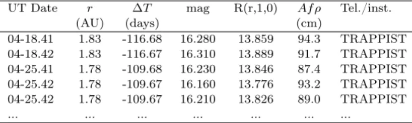
Table A1. R-band Photometry. Measured within an aperture with radius ρ 10,000 km. Full table available online, first 5 rows given as an example.

UT Date r ∆T mag R(r,1,0) Af ρ Tel./inst.

(AU) (days) (cm) 04-18.41 1.83 -116.68 16.280 13.859 94.3 TRAPPIST 04-18.42 1.83 -116.67 16.310 13.889 91.7 TRAPPIST 04-25.41 1.78 -109.68 16.230 13.846 87.4 TRAPPIST 04-25.42 1.78 -109.67 16.160 13.776 93.2 TRAPPIST 04-25.42 1.78 -109.67 16.210 13.826 89.0 TRAPPIST ... ... ... ... ... ... ...

Jester S., et al., 2005, AJ, 130, 873 Le Roy L., et al., 2015, A&A, 583, A1 Luspay-Kuti A., et al., 2015, A&A, 583, A4

Marcus J. N., 2007, International Comet Quarterly, 29, 119 Meech K. J., Svoreň J., 2004, in Festou M. C., Keller H. U.,

Weaver H. A., eds, , Comets II. University of Arizona Press, pp 317–335

Opitom C., Jehin E., Manfroid J., Hutsemékers D., Gillon M., Magain P., 2015, A&A, 574, A38

Piascik A. S., Steele I. A., Bates S. D., Mottram C. J., Smith R. J., Barnsley R. M., Bolton B., 2014, in Ground-based and Airborne Instrumentation for Astronomy V. p. 91478H, doi:10.1117/12.2055117

Roeser S., Demleitner M., Schilbach E., 2010, AJ, 139, 2440 Schleicher D. G., 2006, Icarus, 181, 442

Schleicher D. G., 2010, AJ, 140, 973

Schleicher D. G., Millis R. L., Birch P. V., 1998, Icarus, 132, 397 Snodgrass C., Tubiana C., Bramich D. M., Meech K., Boehnhardt

H., Barrera L., 2013, A&A, 557, A33 Snodgrass C., et al., 2016, A&A, 588, A80

Steele I. A., et al., 2004, in Oschmann Jr. J. M., ed., Proc. SPIEVol. 5489, Ground-based Telescopes. pp 679–692, doi:10.1117/12.551456

Steele I. A., Mottram C. J., Smith R. J., Barnsley R. M., 2014, in High Energy, Optical, and Infrared Detectors for Astronomy VI. p. 915428, doi:10.1117/12.2056602

Steele I. A., et al., 2016, MNRAS, 460, 4268

Strassmeier K. G., et al., 2004, Astronomische Nachrichten, 325, 527

Strassmeier K. G., et al., 2010, Advances in Astronomy, 2010, 970306

Vincent J.-B., Lara L. M., Tozzi G. P., Lin Z.-Y., Sierks H., 2013, A&A, 549, A121

Vincent J.-B., A’Hearn M. F., Lin Z.-Y., El-Maary M. R., Pajola M., Osiris Team 2016, MNRAS, submitted

Zacharias N., Finch C. T., Girard T. M., Henden A., Bartlett J. L., Monet D. G., Zacharias M. I., 2013, AJ, 145, 44

APPENDIX A: PHOTOMETRY

This appendix gives all R-band photometry from the robotic telescopes mentioned in this paper. All values are based on an aperture with radius ρ = 10,000 km at the distance of the comet. Where the telescopes used an SDSS-r filter, a colour correction of -0.2105 has been applied. Heliocentric distance (r) and time from perihelion (∆T ) are given, together with the apparent magnitude as well as the magnitude corrected to unit geocentric distance and zero phase angle, using β = 0.02 mag. deg.−1. The Af ρ quantity is given in cm, without any correction for phase angle in this case.

This paper has been typeset from a TEX/LATEX file prepared by the author.