arXiv:0810.0545v1 [astro-ph] 2 Oct 2008
Phase Referencing in Optical Interferometry
Mercedes E. Filho
a, Paulo Garcia
a,b, Gilles Duvert
c, Gaspard Duchene
d, Eric Thiebaut
e, John
Young
f, Olivier Absil
g, Jean-Phillipe Berger
g, Thomas Beckert
h, Sebastian Hoenig
h, Dieter
Schertl
h, Gerd Weigelt
h, Leonardo Testi
i, Eric Tatuli
i, Virginie Borkowski
j, Micha¨el de Becker
j, Jean Surdej
j, Bernard Aringer
k, Joseph Hron
k, Thomas Lebzelter
k, Andrea Chiavassa
l,
Romano Corradi
l, Tim Harries
ma
Centro de Astrofisica da Universidade do Porto, Rua das Estrelas, 4150-762 Porto, Portugal
b
Departamento de Engenharia F´ısica, Faculdade de Engenharia, Universidade do Porto,
Portugal
c
Laboratoire d’Astrophysique de Grenoble, Observatoire de Grenoble, BP 53, 38041 Grenoble
Cedex 9, France
d
UC Berkeley, Astronomy Department, 601 Campbell Hall, Berkeley CA 94720-3411, USA
e
Observatoire de Lyon, 9 Av. Charles Andr´e, 69561 Saint Genis Laval Cedex, France
f
Cavendish Laboratory, Madingley Road, Cambridge CB3 OHE, UK
g
Universit´e J. Fourier, CNRS, Laboratoire d’Astrophysique de Grenoble, UMR 5571, France;
h
Max-Planck Institute for Radioastronomy, Bonn, Germany;
i
INAF/Osservatorio di Astrofisica di Arcetri, Italy;
j
Institute of Astrophysics and Geophysics, Li`ege, Belgium;
k
Institute of Astrophysics of the University of Wien, Austria;
l
Groupe de Recherche en Astronomie et Astrophysique du Languedoc, Montpellier, France;
m
School of Physics, University of Exeter, UK;
ABSTRACT
One of the aims of next generation optical interferometric instrumentation is to be able to make use of information contained in the visibility phase to construct high dynamic range images.
Radio and optical interferometry are at the two extremes of phase corruption by the atmosphere. While in radio it is possible to obtain calibrated phases for the science objects, in the optical this is currently not possible. Instead, optical interferometry has relied on closure phase techniques to produce images. Such techniques allow only to achieve modest dynamic ranges. However, with high contrast objects, for faint targets or when structure detail is needed, phase referencing techniques as used in radio interferometry, should theoretically achieve higher dynamic ranges for the same number of telescopes.
Our approach is not to provide evidence either for or against the hypothesis that phase referenced imaging gives better dynamic range than closure phase imaging. Instead we wish to explore the potential of this technique for future optical interferometry and also because image reconstruction in the optical using phase referencing techniques has only been performed with limited success.
We have generated simulated, noisy, complex visibility data, analogous to the signal produced in radio in-terferometers, using the VLTI as a template. We proceeded with image reconstruction using the radio image reconstruction algorithms contained in aips imagr (clean algorithm). Our results show that image reconstruc-tion is successful in most of our science cases, yielding images with a 4 milliarcsecond resolureconstruc-tion in K band.
We have also investigated the number of target candidates for optical phase referencing. Using the 2MASS point source catalog, we show that there are several hundred objects with phase reference sources less than 30 arcseconds away, allowing to apply this technique.
Keywords: optical interferometry
Further author information: (Send correspondence to M. E. F.) M. E. F.: E-mail: [email protected], Telephone: +351 6089 853
1. INTRODUCTION
An ideal interferometer will measure the complex visibility of an astronomical object. Image reconstruction deals with inverting the visibility information into an image, given poor Fourier plane sampling and limited phase information.
In an array of N telescopes, signals are combined in 12 × N × (N-1) pairs or baselines to obtain 12 × N ×
(N-1) measurements called complex visibilities. These visibilities are related to the object brightness distribution via the van Cittert-Zernike theorem:
V(u, v) =R R I(x, y) exp[−2 π i (ux + vy)]dx dy
where x and y are angular displacements on the plane of the sky with the phase center as origin, I(x,y) is the brightness distribution of the target and u and v are the position vectors of the baselines projected on a plane perpendicular to the source direction, which together define the uv plane. In practical terms, the better the sampling of the uv plane in terms of baseline length, position angle, and number of measurements, the more faithful the reconstructed image will be relative to the true brightness distribution.
Radio-type observations are performed by measuring the amplitudes (modulus) and the phases (argument) of the complex visibilities:
V(u, v) = A exp(i φ)
Image reconstruction using the modulus and argument of the visibility function is called phase referencing image reconstruction and is widely used in radio astronomy. Studies of this type were previously attempted by Masoni (2006), Masoni et al. (2005) and Weigelt et al. (2008; private communication).
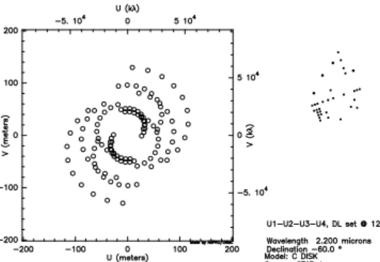
2. ARRAY CONFIGURATION
Telescope configurations are an essential part of the image reconstruction process. We began by identifying array configurations that allowed the most uniform uv coverage:
Figure 1. 4 UT × 1 night configuration.
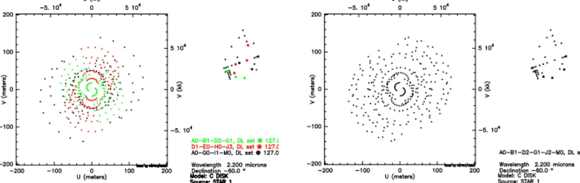
• 4 UTs × 1 night - the chosen configuration when observing very faint sources (Fig. 1); • 4 ATs × 3 nights - the case where there is a small number of telescopes (Fig. 2);
• 6 ATs × 1 night - a 6 telescope extended configuration with one night observation; has less uv points than the 4 AT x 3 nights configuration but comparable uv coverage (Fig. 3).
Figure 2. 4 AT × 3 night configuration (left). 6 AT × 1 night configuration (right).
3. NOISE MODEL
The noise model estimates the uncertainties on the visibility amplitudes and phases assuming an instrument following a multi-axial recombination scheme with a fringe tracker (FT; Jocou et al. 2007).
The quantity we procure is the total number of detected photoevents per integration time per pixel per baseline in the interferometric channel:
Ni =NNpixtotal∗N∗f
base
where f is the fraction of the beam that gores into the interferometric channel (90%), Npix is the number of
pixels needed to read the interferometric channel (600), Nbaseis the number of baselines and Ntotal is the total
number of detected photevents per integration time per pixel in all channels:
Ntotal= F0∗ 10−0.4mag∗ tint∗ Ntel∗ π ∗ R2∗ ∆λ ∗ trans ∗ Strehl
Here F0 is the photon flux of a zeroth magnitude star (Jocou et al. 2007), mag is the object magnitude in the
observing band, tint is the integration time, Ntel is the number of telescopes (6 or 4), R is the radius of the
telescopes (4.1 for UTs and 0.9 for ATs) assumed for simplification to have no central hole, ∆λ is the spectral bandwidth (chosen), trans is the total instrument transmission including quantum efficiency (Jocou et al. 2007), and Strehl is the Strehl ratio and depends on wavelength (Jocou et al. 2007).
Therefore, the total number of detected photevents in the interferometric channel is:
Ni= Ni∗ Npix∗ Nint
where Nint is the number of independent integrations (depends on magnitude and FT presence).
The object intrinsic visibility, V , must be corrected for the instrumental visibility loss (80%) and the instru-mental visibility loss induced by the FT (90%). The correlated flux per baseline is therefore:
Fcor= Ni∗ V
′
2
and finally the error in visibility is given by:
errorV =pFcor+ Nint∗ Npix∗ σ2
4. UVFITS FILE GENERATION
UVFITS is the file format in which radio astronomical data are written and used for phase referencing image reconstruction. UVFITS format is designed so that different categories of information are stored in distinct tables within a file and can be cross-referenced one to another. Each UVFITS file table stores specific parameters that include important interferometric observables and system information.
Key science images were generated and provided by the science case groups (Garcia et al. 2007). Using
aspro, an image simulation tool originally created for IRAM, and the configurations above, K band ”images”
of the sources were created assuming that all sources were observed at the fixed declination of −60 degrees. It was assumed also that during the night, the telescope configurations would remain fixed and that one calibrated uv point per baseline should be obtained every hour. The actual on-source integration time is, however, 10-15 minutes per hour due to overheads. The total integration time assumes an entire transit (9 hours).
5. PHASE REFERENCING THEORY
A radio interferometer works by phase referencing. The interferometer observes a science target and records the visibility modulus and phase for each baseline. It also observes a reference target used to calibrate the visibility modulus and phase for atmospheric variations. Therefore, as opposed to conventional optical interferometry, phase referencing makes use of crucial information contained in the phases to recover the brightness distribution of a source. s’ s I (s) obs (x,y) Figure 3.
Given an incoherent source, the observed brightness distribution in a direction ~s′ is given by:
Iobs(~s′) = Iobs(x, y) = P SF (x, y) ∗ Itrue(x, y) + N (x, y)
where PSF(x,y) is the instrumental point spread function, Itrue(x,y) is the true object brightness distribution,
N(x,y) is the noise and the asterisk denotes convolution.
In practice, interferometry does not make measurements in the image plane but in Fourier space. The relevant quantity is called the complex visibility and is measured at each uv point, the position vector of the baseline on a plane perpendicular to the source direction:
Vobs(u, v) = S(u, v) × Vtrue(u, v) + N′(u, v)
where S(u,v), the sampling function, is the Fourier transform of the PSF(x,y), Vtrue(x,y), the true visibility, is
the Fourier transform of the true brightness distribution Itrue(x,y) and N’(u,v) is the noise in the Fourier space.
The van Cittert-Zernike theorem states that the true brightness distribution can be obtained by the inverse Fourier transform and deconvolution of the observables:
Itrue
(x, y) ∗ P SF (x, y) =R R Vtrue
(u, v) × S(u, v) exp [2πi(ux + vy)] du dv
The role of image reconstruction is to obtain the best approximation, Iaprox(x,y) ∼ Iobs(x,y) ∼ Itrue(x,y), to
the true brightness distribution.
In radio-like phase referencing image reconstruction, the data are gridded, interpolated and inverse Fourier transformed to yield a model representation of the sky:
Idirty(x, y) = Iaprox
(x, y) ∗ P SFdirty(x, y) + N (x, y)
where Idirty(x, y) is called the dirty map and P SFdirty(x, y) is called the dirty beam.
The NRAO Astronomical Image Processing System (aips), is a baseline-based reconstruction method used in radio interferometry. The UVFILES generated by aspro were imported into aips. We have tested the results using the clean algorithm (H¨ogbom 1974), which corrects for the effect of poor Fourier plane sampling. clean grids, Fourier transforms and deconvolves the dirty beam from the dirty image in an iterative fashion given an initial guess for the beam and the brightness distribution. clean then finds peaks in the residual image and subtracts δ functions of the appropriate strength at those positions. The final map is a convolution of all the δ functions with a clean beam plus the residual map.
6. IMAGE ANALYSIS
In order to compare the reconstructed with the synthetic images, aspro was used to generate the point spread functions (PSF) for the 6 AT × 1 night, 4 AT × 3 nights and 4 UT × 1 night configurations (Table 1). The synthetic images were then convolved with a Gaussian of the measured PSF parameters (iraf program gauss).
Table 1. PSF parameters. Col. 1: Configuration. Col. 2: Full width at half maximum. Col. 3: Dispersion, σ = F W HM/2.35. Col. 4: Elllipticity, e = a−b
a+b, where
a is the major and b the minor axis. Col. 5: Axis ratio, r = 1−e
1+e. Col. 6: Position angle of the minor axis.
Configuration FWHM σ e r PA
4 UT × 1 night 4.45 1.89 0.08 0.85 −9.0· 4 AT × 3 nights 3.51 1.49 0.38 0.45 −83.0· 6 AT × 1 night 5.17 2.20 0.42 0.41 −85.0·
Relative astrometry information was obtained for the images using ds9. Photometry of the image components was performed using iraf procedure phot. SN R is the ratio of the mean pixel value to the standard deviation meansured on the reconstructed images.
7. PHASE REFERENCING IMAGE RECONSTRUCTION
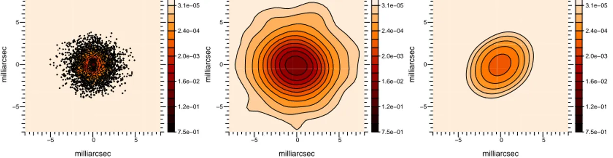
Table 2. AGN. Diameter units are pixels. Image 4 UT aips4 UT flux sublimation 84.9% 97.0% flux torus 15.1% 3.0% ratio 5.6 32.3 sublimation diameter 50 45 torus diameter 260 -SNR - 89
−5 0 5 −5 0 5 7.5e−01 1.2e−01 1.6e−02 2.0e−03 2.4e−04 3.1e−05 milliarcsec milliarcsec −5 0 5 −5 0 5 7.5e−01 1.2e−01 1.6e−02 2.0e−03 2.4e−04 3.1e−05 milliarcsec milliarcsec −5 0 5 −5 0 5 7.5e−01 1.2e−01 1.6e−02 2.0e−03 2.4e−04 3.1e−05 milliarcsec milliarcsec
Figure 4. A simulated AGN with jet component and torus, 0.1 mas/pixel sampling; convolved image, 4 UT × 1 night configuration, 0.5 mas/pixel sampling, 4.45 mas FWHM resolution; aips reconstruction 4 UT × 1 night configuration, 0.1 mas/pixel sampling. −20 −10 0 10 20 −20 −10 0 10 20 7.5e−01 1.2e−01 1.6e−02 2.0e−03 2.4e−04 3.1e−05 3.8e−06 milliarcsec milliarcsec −20 −10 0 10 20 −20 −10 0 10 20 7.5e−01 1.2e−01 1.6e−02 2.0e−03 2.4e−04 3.1e−05 milliarcsec milliarcsec −20 −10 0 10 20 −20 −10 0 10 20 7.5e−01 1.2e−01 1.6e−02 2.0e−03 2.4e−04 3.1e−05 3.8e−06 milliarcsec milliarcsec −20 −10 0 10 20 −20 −10 0 10 20 7.5e−01 1.2e−01 1.6e−02 2.0e−03 2.4e−04 3.1e−05 milliarcsec milliarcsec −20 −10 0 10 20 −20 −10 0 10 20 7.5e−01 1.2e−01 1.6e−02 2.0e−03 2.4e−04 3.1e−05 3.8e−06 milliarcsec milliarcsec
Figure 5. A low mass evolved star system with an outflow, 0.1 mas/pixel sampling; convolved image, 4 AT × 3 nights configuration, 0.5 mas/pixel sampling, 3.51 mas FWHM resolution; aips reconstruction 4 AT × 3 nights configuration, 0.1 mas/pixel sampling; convolved image, 6 AT × 1 night configuration, 0.5 mas/pixel sampling, 5.17 mas FWHM resolution; aipsreconstruction 6 AT × 1 night configuration, 0.1 mas/pixel sampling.
Table 3. Evolved Star. Diameter units are pixels.
Image 4 AT 3 aips4 AT 3 Image 6 AT aips6 AT
flux star 21.9% 29.4% 21.9% 28.7%
flux wind 78.1% 70.6% 78.1% 71.3%
ratio star/wind 0.3 0.4 0.3 0.4
inner wind diameter 50 × 35 50 × 35 50 × 35 50 × 35 outer wind diameter 100 × 85 100 × 85 100 × 85 100 × 85
SNR - 46 - 23
8. DISCUSSION
If we compare the reconstructed images with the convolved images, we see that the phase referencing image reconstruction has yielded good results. Most of the flux is recovered in the individual image elements and the
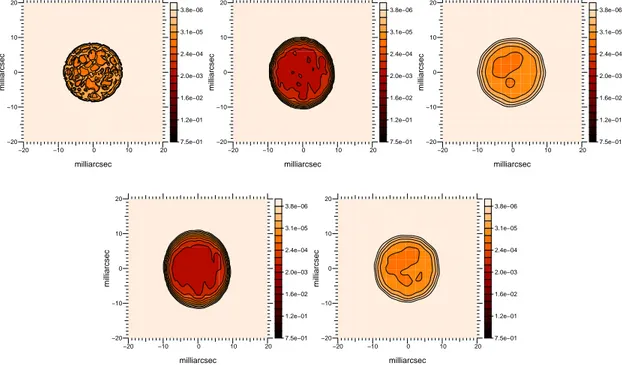
−20 −10 0 10 20 −20 −10 0 10 20 7.5e−01 1.2e−01 1.6e−02 2.0e−03 2.4e−04 3.1e−05 3.8e−06 milliarcsec milliarcsec −20 −10 0 10 20 −20 −10 0 10 20 7.5e−01 1.2e−01 1.6e−02 2.0e−03 2.4e−04 3.1e−05 3.8e−06 milliarcsec milliarcsec −20 −10 0 10 20 −20 −10 0 10 20 7.5e−01 1.2e−01 1.6e−02 2.0e−03 2.4e−04 3.1e−05 3.8e−06 milliarcsec milliarcsec −20 −10 0 10 20 −20 −10 0 10 20 7.5e−01 1.2e−01 1.6e−02 2.0e−03 2.4e−04 3.1e−05 3.8e−06 milliarcsec milliarcsec −20 −10 0 10 20 −20 −10 0 10 20 7.5e−01 1.2e−01 1.6e−02 2.0e−03 2.4e−04 3.1e−05 3.8e−06 milliarcsec milliarcsec
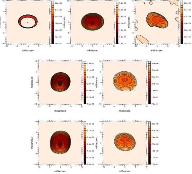
Figure 6. A simulated stellar surface of a M giant, 0.1 mas/pixel sampling; convolved image, 4 AT × 3 nights configuration, 0.5 mas/pixel sampling, 3.51 mas FWHM resolution; aips reconstruction 4 AT × 3 nights configuration, 0.1 mas/pixel sampling, SN R = 34; convolved image, 6 AT × 1 night configuration, 0.5 mas/pixel sampling, 5.17 mas FWHM resolution; aipsreconstruction 6 AT × 1 night configuration, 0.1 mas/pixel sampling, SNR = 24.
−20 −10 0 10 20 −20 −10 0 10 20 7.5e−01 1.2e−01 1.6e−02 2.0e−03 2.4e−04 3.1e−05 3.8e−06 0.0e+00 milliarcsec milliarcsec −20 −10 0 10 20 −20 −10 0 10 20 7.5e−01 1.2e−01 1.6e−02 2.0e−03 2.4e−04 3.1e−05 3.8e−06 0.0e+00 milliarcsec milliarcsec −20 −10 0 10 20 −20 −10 0 10 20 7.5e−01 1.2e−01 1.6e−02 2.0e−03 2.4e−04 3.1e−05 3.8e−06 0.0e+00 milliarcsec milliarcsec
Figure 7. A simulated stellar surface of a supergiant, 0.1 mas/pixel sampling; convolved image, 6 AT × 1 night con-figuration, 0.5 mas/pixel sampling, 5.17 mas FWHM resolution; aips reconstruction 6 AT × 1 night concon-figuration, 0.1 mas/pixel sampling, SN R = 216.
Table 4. Microlensing. Distance units are pixels. Image 4 UT aips4 UT A flux 12.8% 12.9% B flux 19.2% 19.6% C flux 68.0% 67.5% ratio C/A 5.3 5.2 ratio C/B 3.5 3.4 distance AC 45 45 distance BC 70 70 distance AB 50 50 SNR - 99
−10 −5 0 5 10 −10 −5 0 5 10 7.5e−01 1.2e−01 1.6e−02 2.0e−03 2.4e−04 3.1e−05 3.8e−06 milliarcsec milliarcsec −10 −5 0 5 10 −10 −5 0 5 10 7.5e−01 1.2e−01 1.6e−02 2.0e−03 2.4e−04 3.1e−05 3.8e−06 milliarcsec milliarcsec −10 −5 0 5 10 −10 −5 0 5 10 7.5e−01 1.2e−01 1.6e−02 2.0e−03 2.4e−04 3.1e−05 3.8e−06 milliarcsec milliarcsec
Figure 8. A simulated microlensing event, 0.1 mas/pixel sampling; convolved image, 4 UT × 1 night configuration, 0.5/pixel sampling, 4.45 mas FWHM resolution; aips reconstruction 4 UT × 1 nights configuration, 0.1 mas/pixel sam-pling. −40 −20 0 20 40 −40 −20 0 20 40 7.5e−01 1.2e−01 1.6e−02 2.0e−03 2.4e−04 3.1e−05 3.8e−06 milliarcsec milliarcsec −40 −20 0 20 40 −40 −20 0 20 40 7.5e−01 1.2e−01 1.6e−02 2.0e−03 2.4e−04 3.1e−05 3.8e−06 milliarcsec milliarcsec −40 −20 0 20 40 −40 −20 0 20 40 7.5e−01 1.2e−01 1.6e−02 2.0e−03 2.4e−04 3.1e−05 3.8e−06 milliarcsec milliarcsec −40 −20 0 20 40 −40 −20 0 20 40 7.5e−01 1.2e−01 1.6e−02 2.0e−03 2.4e−04 3.1e−05 0.0e+00 milliarcsec milliarcsec −40 −20 0 20 40 −40 −20 0 20 40 7.5e−01 1.2e−01 1.6e−02 2.0e−03 2.4e−04 3.1e−05 3.8e−06 milliarcsec milliarcsec −40 −20 0 20 40 −40 −20 0 20 40 7.5e−01 1.2e−01 1.6e−02 2.0e−03 2.4e−04 3.1e−05 3.8e−06 milliarcsec milliarcsec
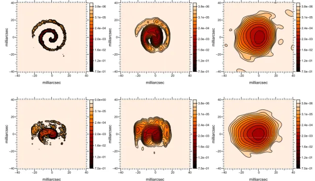
Figure 9. A simulated image of the pinwheel nebula at 0 degree inclination, 1.0 mas/pixel sampling; convolved image, 1.0 mas/pixel sampling, 5.17 FWHM, 6 AT × 1 night configuration; aips reconstruction 6 AT × 1 night configuration, 0.1 mas/pixel sampling. A simulated image of the pinwheel nebula at 60 degree inclination, 1.0 mas/pixel sampling; convolved image, 1.0 mas/pixel sampling, 5.17 FWHM, 6 AT × 1 night configuration; aips reconstruction 6 AT × 1 night configuration, smoothness regularization, 0.1 mas/pixel sampling.
Table 5. Pinwheel
Angle Image 6 AT aips6 AT SNR inner spiral 0 deg 24 × 30 24 × 24 281 inner spiral 60 deg 24 × 24 24 × 22 404
astrometry is excellent. A clear example of this is the reconstructed stellar surface images. Most of the flux is recovered in a compact region and careful inspection of the reconstructed images shows correspondence with individual brightness regions in the convolved image. The edges of the stellar surface are also well reproduced.
For an array of N telescopes, the total number of measurements per observing night per integration point
(moduli plus phase over each baseline) in phase referencing is N × (N − 1) compared to (N −1)2 × (
3
2N − 2) closure
−10 −5 0 5 10 −10 −5 0 5 10 7.5e−01 1.2e−01 1.6e−02 2.0e−03 2.4e−04 3.1e−05 3.8e−06 milliarcsec milliarcsec −10 −5 0 5 10 −10 −5 0 5 10 7.5e−01 1.2e−01 1.6e−02 2.0e−03 2.4e−04 3.1e−05 3.8e−06 milliarcsec milliarcsec −10 −5 0 5 10 −10 −5 0 5 10 7.5e−01 1.2e−01 1.6e−02 2.0e−03 2.4e−04 3.1e−05 3.8e−06 milliarcsec milliarcsec −10 −5 0 5 10 −10 −5 0 5 10 7.5e−01 1.2e−01 1.6e−02 2.0e−03 2.4e−04 3.1e−05 3.8e−06 milliarcsec milliarcsec −10 −5 0 5 10 −10 −5 0 5 10 7.5e−01 1.2e−01 1.6e−02 2.0e−03 2.4e−04 3.1e−05 3.8e−06 milliarcsec milliarcsec −10 −5 0 5 10 −10 −5 0 5 10 7.5e−01 1.2e−01 1.6e−02 2.0e−03 2.4e−04 3.1e−05 3.8e−06 milliarcsec milliarcsec −10 −5 0 5 10 −10 −5 0 5 10 7.5e−01 1.2e−01 1.6e−02 2.0e−03 2.4e−04 3.1e−05 3.8e−06 milliarcsec milliarcsec
Figure 10. A simulated stellar surface of the structure of inner disks surrounding YSOs, 0.1 mas/pixel sampling; convolved image, 4 UT × 1 night configuration, 0.5 mas/pixel sampling, 4.45 mas FWHM resolution; aips reconstruction 4 UT × 1 night configuration, 0.1 mas/pixel sampling; convolved image, 4 AT × 3 nights configuration, 0.5 mas/pixel sampling, 3.51 mas FWHM resolution; aips reconstruction 4 AT × 3 nights configuration, 0.1 mas/pixel sampling; convolved image, 6 AT × 1 night configuration, 0.5 mas/pixel sampling, 5.17 mas FWHM resolution; aips reconstruction 6 AT × 1 night configuration, 0.1 mas/pixel sampling.
Table 6. YSO. Diameter units are pixels.
Image 4 UT aips4 UT Image 4 AT 3 aips4 AT 3 Image 6 AT aips6 AT
flux star 15.7% - 18.1% - 18.1% 16.7%
flux disk 84.3% - 81.9% - 81.9% 83.3%
ratio 0.2 - 0.2 - 0.2 0.2
outer diameter 60 × 40 60 × 40 70 × 60 70 × 60 80 × 70 80 × 70
SNR - 1 - 184 - 530
6 measured parameters for phase closure observations and 12 for phase referencing. Therefore, phase referenced reconstructed images should theoretically be more rigorous.
9. OBSERVABLE OBJECTS
In order to perform real time phase referencing observations, it is necessary to have a phase reference source no more than 30” away from the target source. For larger distances, the atmospheric pistons become distinct and the calibration incorrect.
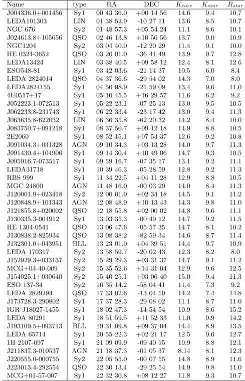
Among the science cases presented, the most crucial in terms of number of phase reference candidates are the AGN, due to their large distances and therefore their K band faintness. We have attempted to quantify the number of AGN for which phase reference imaging is possible by using the V´eron-Cetty & V´eron (2006) catalog which contains AGNs, QSOs and BL Lac objects. Firstly, we constrained the science targets to those visible to the VLTI: targets were chosen to be between +20 and −90 degree declination. We then searched the 2MASS point source catalog for a nearby (less than 30” from the science target) bright star suitable for both AO wavefront sensing and fringe tracking (i.e., star mangitudes K <10, R <16). Science targets are listed in Table 7.
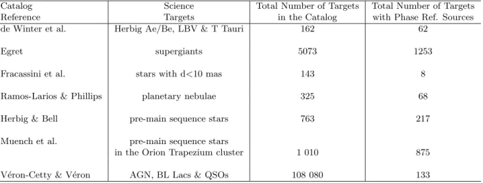
We have also investigated the number of phase reference targets available from a series of stellar catalogs. No trimming of objects for observability (southern hemisphere or target magnitude) was done. The following catalogs were searched: the de Winter et al. (2001) catalog of southern emission line objects mainly containing Herbig Ae/Be stars and some B[e], LBV and TTauri stars; the Egret (1980) catalog of supergiants; the Fracassini et al. (1994) catalog of stellar radii trimmed to objects with diameters of at least 10 mas; the Ramos-Larios & Phillips (2005) catalog of planetary nebulae; the Herbig & Bell (1995) catalog of pre-main-sequence stars; the Muench et al. (2002) catalog of pre-main-sequence stars in the Orion Trapezium cluster. We have searched for appropriate phase reference 2MASS point sources with K band magnitudes between 9 and 11 less then 30” away from the targets. The results are presented in Table 8 and highlight the potencial of phase reference imaging.
10. CONCLUSIONS
Theoretically it is found that phase reference image reconstruction should yield more rigourous images than the classical phase closure method used in optical interferometry, not only because longer integrations times are allowed, but also because the former method measures information related to the visibility phase.
We wished to explore the potential of phase referencing in optical interferometry. We have generated sim-ulated, noise visbility amplitudes and phases using the VLTI as a template and reconstructed images with the classic radio interferometry algorithm clean contained in the aips package. Our results show that with this method we will be able to reconstruct images of diverse sources with a spatial resolution of about 4 milliarcseconds in K band.
We have also compiled a list of target sources for which optical phase referencing is possible and found several hundred candidates.
11. ACKNOWLEDGMENTS
We would like to thank J. Brinchmann for his help with the phase reference sources. MEF is supported by
the Funda c˜ao para a Ciˆencia e a Tecnologia through the research grant SFRH/BPD/36141/2007. PJVG and
MEF were supported in part by the Funda c˜ao para a Ciˆencia e a Tecnologia through projects
PTDC/CTE-AST/68915/2006 and PTDC/CTE-AST/65971/2006 from POCI, with funds from the European programme FEDER.
12. REFERENCES
Egret, D. 1980, Bulletin d’Information du Centre de Donnees Stellaires, 18, 82
Fracassini, M., Pasinetti-Fracassini, L. E., Pastori, L., & Pironi, R. 1994, VizieR Online Data Catalog, 2155, 0 Garcia, P. et al. 2007, in doc. VLT-SPE-VSI-15870-4335, issue 1.0 in VSI Phase A Document Package, Science Cases
Table 7. Science target list of all southern (declination +20 to -90◦) AGNs in the V´eron-Cetty & V´eron catalog (2006)
with a bright star (K < 10 and R < 16) in their isoplanatic patch (i.e., star separation < 30 arcsec). These nearby stars are suitable for both AO wavefront sensing and fringe tracking. The Kcore magnitudes are the K magnitudes from the
2mass catalog, the Kstar and Rstar magnitudes are the magnitudes of the nearby stars.
Name type RA DEC Kcore Kstar Rstar
J004336.0+001456 Sy1 00 43 36.0 +00 14 56 14.6 9.4 10.7 LEDA101303 LIN 01 38 52.9 -10 27 11 13.6 8.5 10.7 NGC 676 Sy2 01 48 57.3 +05 54 24 11.1 8.6 10.1 J024613.8+105656 QSO 02 46 13.8 +10 56 56 13.7 9.0 10.9 NGC1204 Sy2 03 04 40.0 -12 20 29 11.4 9.1 10.0 HE 0324-3652 QSO 03 26 01.0 -36 41 49 13.9 9.7 12.8 LEDA13424 LIN 03 38 40.5 +09 58 12 12.4 8.1 12.6 ESO548-81 Sy1 03 42 03.6 -21 14 37 10.5 6.0 8.4 LEDA 2824014 QSO 04 37 36.6 -29 54 02 14.3 7.0 8.0 LEDA2824155 Sy1 04 56 08.9 -21 59 09 13.4 9.6 11.0 4U0517+17 Sy1 05 10 45.5 +16 29 57 11.6 6.2 9.2 J052223.1-072513 Sy1 05 22 23.1 -07 25 13 13.0 9.5 10.5 J062233.8-231743 Sy1 06 22 33.4 -23 17 42 13.0 9.4 11.3 J063635.8-622032 LIN 06 36 35.8 -62 20 32 14.2 8.4 10.0 J083750.7+091218 Sy1 08 37 50.7 +09 12 18 14.9 8.8 10.5 2E2060 Sy1 08 52 15.1 +07 53 37 12.6 9.2 10.8 J091034.3+031328 AGN 09 10 34.3 +03 13 28 14.0 9.7 11.3 J091430.4+104906 Sy1 09 14 30.4 +10 49 06 14.7 9.3 10.5 J095916.7-073517 Sy1 09 59 16.7 -07 35 17 13.1 9.2 11.1 LEDA31718 Sy1 10 39 46.3 -05 28 59 12.8 9.2 11.3 RBS 999 Sy1 11 34 22.5 +04 11 28 12.9 8.8 10.5 MGC 24800 AGN 11 48 16.0 -00 03 29 14.0 8.4 11.3 J120001.9+023418 Sy2 12 00 01.9 +02 34 18 14.5 9.1 11.2 J120848.9+101343 AGN 12 08 48.9 +10 13 43 14.3 9.8 11.0 J121855.8+020002 QSO 12 18 55.8 +02 00 02 14.8 9.6 11.1 J130335.3-004912 Sy1 13 03 35.3 -00 49 12 14.7 9.2 11.5 HE 1304-0541 QSO 13 06 47.6 -05 57 35 14.7 8.1 10.2 J130838.2-825934 QSO 13 08 38.2 -82 59 34 14.6 8.7 11.4 J132301.0+043951 BLL 13 23 01.0 +04 39 51 14.4 9.7 10.9 LEDA 170317 Sy2 13 58 59.7 -20 02 43 12.3 8.2 8.0 J152929.3+033137 Sy2 15 29 29.3 +03 31 37 14.7 9.1 11.2 MCG+03-40-009 Sy2 15 35 52.6 +14 31 04 12.9 9.6 12.5 J154025.1+030640 Sy2 15 40 25.1 +03 06 40 15.0 9.4 11.3 ESO 137-34 Sy2 16 35 14.2 -58 04 41 11.4 7.3 9.2 LEDA 2829294 QSO 17 33 02.6 -13 04 50 14.2 7.4 14.8 J173728.3-290802 Sy1 17 37 28.3 -29 08 02 11.1 8.7 11.0 IGR J18027-1455 Sy1 18 02 47.3 -14 54 54 10.9 8.6 15.2 LEDA 86291 Sy1 18 51 59.5 +11 52 33 11.0 9.9 14.2 J193109.5+093713 BLL 19 31 09.8 +09 37 04 14.4 8.9 13.5 LEDA 65714 Sy1 20 55 22.3 +02 21 17 12.5 9.6 12.7 1H 2107-097 Sy1 21 09 09.9 -09 40 15 10.9 8.8 12.1 J211837.3-010537 AGN 21 18 37.3 -01 05 37 8.14 8.1 12.3 J220555.0-000755 Sy2 22 05 55.0 -00 07 55 14.8 8.9 11.6 J223013.4-292554 QSO 22 30 13.4 -29 25 54 14.9 9.8 11.0 MCG+01-57-007 Sy1 22 32 30.8 +08 12 27 11.8 9.3 10.7
H¨ogbom, J. A., 1974, A&AS, 15, 417
Jocou, L. et al. 2007, in doc. VLT-SPE-VSI-15870-4335, issue 1.0 in VSI Phase A Document Package, System Design
Table 8. Science target list with a bright star (9<K<11) in their isoplanatic patch (i.e., star separation < 30 arcsec). These nearby stars are suitable for fringe tracking.
Catalog Science Total Number of Targets Total Number of Targets Reference Targets in the Catalog with Phase Ref. Sources de Winter et al. Herbig Ae/Be, LBV & T Tauri 162 62
Egret supergiants 5073 1253
Fracassini et al. stars with d<10 mas 143 8
Ramos-Larios & Phillips planetary nebulae 325 68
Herbig & Bell pre-main sequence stars 763 217
Muench et al. pre-main sequence stars
in the Orion Trapezium cluster 1 010 875
V´eron-Cetty & V´eron AGN, BL Lacs & QSOs 108 080 133
Masoni, L. et al. 2005, Astr. Nachr., 326, 566
Muench, A. A., Lada, E. A., Lada, C. J., & Alves, J. 2002, ApJ, 573, 366 Ramos-Larios, G., & Phillips, J. P. 2005, MNRAS, 357, 732
V´eron-Cetty, M. -P. & V´eron, P. 2006, A&A, 455, 773
de Winter, D., van den Ancker, M. E., Maira, A., Th´e, P. S., Djie, H. R. E. T. A., Redondo, I., Eiroa, C., & Molster, F. J. 2001, A&A, 380, 609