TH `ESE
TH `ESE
En vue de l’obtention du
DOCTORAT DE L’UNIVERSIT´E DE TOULOUSE
D´elivr´e par : l’Universit´e Toulouse 3 Paul Sabatier (UT3 Paul Sabatier)
Pr´esent´ee et soutenue le 14/10/2016 par :
Teodora SZASZ
Advanced beamforming techniques in ultrasound imaging and the associated inverse problems
Techniques avanc´ees de formation de voies en imagerie ultrasonore et probl`emes inverses associ´es
JURY
Jean-Louis DILLENSEGER Maˆıtre de conf´erences, Universit´e de Rennes 1 Rapporteur Nicole VINCENT Professeur, Universit´e Paris Descartes Rapporteur Philippe DELACHARTRE Professeur, INSA Lyon Examinateur Mircea-Florin VAIDA Professeur, Universit´e Technique de Cluj-Napoca Examinateur Adrian BASARAB Maˆıtre de conf´erences, Universit´e Paul Sabatier Directeur de Th`ese Denis KOUAM´E Professeur, Universit´e Paul Sabatier Directeur de Th`ese
´Ecole doctorale et sp´ecialit´e :
MITT : Image, Information, Hyperm´edia
Unit´e de Recherche :
Institut de Recherche en Informatique de Toulouse (UMR 5505)
Directeur(s) de Th`ese :
Adrian BASARAB et Denis KOUAM ´E
Rapporteurs :
Firstly, I would like to thank Paul Sabatier University members and the doctoral school, EDMITT, for offering me the financial support during these three years of PhD. I am thankful to IRIT laboratory that offered me space and support during the master internship and PhD period. Also, I am grateful to Technical University of Cluj-Napoca, Romania for the financial support through the Erasmus scholarship during the master internship. The internship gave me the opportunity to meet my PhD supervisors, Dr. Adrian Basarab and Prof. Denis Kouamé and to discover the fascinating world of ultrasound imaging.
I will never be able to express in words the gratitude for the permanent support and help of my PhD supervisors Dr. Adrian Basarab and Prof. Denis Kouamé. They helped me integrate in their team and taught me the main concepts of ultrasound imaging and how to approach a PhD thesis. I really appreciate their time spent on correcting my articles. I know that, at the beginning, they probably spent more time on corrections than if they were writing the articles by themselves. But they knew that this is the only way I will be able to learn the right way of writing research articles. Also, I really appreciate their patience during my "learning french" process. I know that at the beginning the meetings in french with them were in a "franglish" language, that sometimes just myself I could understand, but they always motivated me to continue and practice doing presentations in french. This was so helpful when I had to do my first oral presentation in french at GRETSI conference in 2015. Thank you again. Now, looking back at these four years (one of internship and three of PhD), I can say, without any hesitation, that they are the best supervisors I could have. They are are experts in ultrasound imaging, amazing managers of the time and resources,
All the results I had during my PhD (and I am quite proud about them) were not been possible without their special help, guidance, and motivation. Thank you again!
I am truly grateful to Prof. Mircea-Florin Vaida for supporting me in my ca-reer since my first year of university at Technical University of Cluj Napoca, Romania. Since almost 10 years he is continuously guiding me in each im-portant step of my career. He offered me the chance to work in a professional research laboratory, at IRIT, and he gave very precious advices, even in the most difficult situations. I really want to thank him for the last days, be-fore my PhD defense, for being near me, encouraging me and motivating me. He always knows how to take out the best of me in critical moments (like preparing a good presentation in 3-4 days, with a terrible jet lag of 7 hours). Prof. Mircea-Florin Vaida is my best example of dedication to the students. He is the only professor I know that is everytime ready to help a good student, no matter of circumstances.
I would also like to thank Dr. Hervé Liebgott and Adeline Bernard from CREATIS laboratory at Lyon for offering me the possibility to work on their US scanners and their precious support during my PhD thesis. Almost all the experimental data in this manuscript was acquired with their US scanners.
Thank you Dr. Zhouye Chen for being in front of me in our office for 3 years. Thank you for being such an amazing colleague and friend. Thank you Rémi Abbal and Renaud Morin for helping me in my first year at IRIT and for being so patient during my "learning french" process. Many thanks to my colleagues and friends NingNing, Rose, Thang, Bérengère, Arturo, and Rémi.
Special thanks to Sébastien for the patience, help, continuously support, and love he offered me during my PhD. Thanks to my friends Julia, Vincent, and Hubert for all the special social moments we spent together.
cross borders that I never thought I will we able to pass. "You are the crack in my world".
The support of my family is endless...Thank you for your love, motivation, and for being such an amazing family. I want to dedicate this thesis to you.
List of Figures xi
List of Tables xvii
Glossary xix
1 Ultrasound imaging 1
1.1 Ultrasound imaging principles . . . 2
1.1.1 Principle of ultrasound imaging . . . 2
1.1.2 Sound propagation in medium . . . 5
1.1.2.1 Reflection and transmission . . . 7
1.1.2.2 Scattering, absorption, and attenuation . . . 8
1.1.2.3 Speckle . . . 9
1.1.3 Transducers . . . 9
1.1.4 Scanning . . . 10
1.1.5 Imaging modalities . . . 11
1.2 Ultrasound image visualization . . . 13
1.2.1 Image visualization modes . . . 14
1.2.2 Image resolution . . . 16
1.2.3 Image quality metrics . . . 17
2 Beamforming in medical ultrasound imaging: State of the art 19
2.1 Focusing . . . 20
2.2 Main ultrasound imaging elements . . . 21
2.3 Data-independent beamforming: DAS . . . 22
2.4 Data-dependent beamforming . . . 24
2.4.1 Capon or minimum variance beamformer . . . 25
2.4.2 Improved MV beamformer approaches . . . 27
2.4.2.1 Diagonal loading . . . 27
2.4.2.2 Coherence factor weighting . . . 28
2.4.2.3 Frequency subbands . . . 30
2.5 Subspace methods: MUSIC . . . 31
2.6 Parametric methods: Maximum Likelihood . . . 31
2.7 Beamspace beamforming . . . 32
2.7.1 Multi-beam beamforming . . . 33
2.8 User parameter-free beamforming approaches: IAA . . . 35
2.9 Compressive sampling beamforming . . . 39
2.10 Beamforming in other domains . . . 39
2.10.1 Mathematical formulation of inverse problems . . . 40
2.10.2 Beamforming as inverse problem in medical ultrasound imaging . 41 3 Strong reflector-based beamforming in medical ultrasound imaging 43 3.1 Introduction . . . 44
3.2 Beamforming with sparse priors . . . 44
3.2.1 Sparse strong reflector model . . . 44
3.2.2 Strong reflector detection and parameter estimation . . . 45
3.2.2.1 1D initialization procedure: . . . 46
3.2.2.2 2D refinement procedure: . . . 48
3.2.3 Final image computation . . . 48
3.3 Experiments . . . 49
3.3.1 Simulated point reflectors . . . 50
3.3.2 Simulated point reflectors and cyst data . . . 52
3.3.3 Simulated cardiac apical view image . . . 52
3.4 Results and discussion . . . 53
3.4.1 Sparsely located point reflectors . . . 53
3.4.2 Point reflectors and cyst data . . . 55
3.4.3 Cardiac apical view image . . . 60
3.4.4 Recorded experimental data . . . 64
3.5 Conclusions . . . 68
4 Beamforming through regularized inverse problems in medical ultra-sound imaging 69 4.1 Introduction . . . 70
4.2 Beamforming through regularized inverse problems . . . 71
4.2.1 Model formulation . . . 71
4.2.2 Beamspace processing . . . 73
4.2.3 Beamforming through regularized inverse problems . . . 74
4.2.3.1 Laplacian statistics through Basis Pursuit (BP) . . . 75
4.2.3.2 Gaussian statistics through Least Squares (LS) . . . 76
4.2.3.3 Elastic-net (EN) regularization . . . 76
4.3 Experiments . . . 77
4.3.1 Parameters for the comparative methods . . . 80
4.3.2 Simulated point reflectors . . . 80
4.3.3 Simulated phantom data . . . 80
4.3.4 Simulated cardiac image . . . 81
4.3.5 In vivo data: carotid . . . 81
4.3.6 In vivo data: thyroid . . . 81
4.4 Results and Discussion . . . 81
4.4.1 Individual point reflectors . . . 82
4.4.2 Simulated hypoechoic cyst . . . 84
4.4.3 Simulated cardiac image . . . 89
4.4.4 In vivo data: carotid . . . 91
4.4.5 In vivo data: healthy thyroid . . . 94
4.4.6 In vivo data: thyroid with tumor . . . 97
5 Beamforming of stable distributed ultrasound images 99
5.1 Acquisition setup . . . 100
5.2 Beamforming of US images modelled as stable random variables . . . 102
5.2.1 Signal model . . . 102
5.2.2 ↵-stable distributions model . . . 103
5.2.3 Model inversion via `p-norm regularization . . . 104
5.3 Results and discussion . . . 105
5.3.1 Simulated data with point reflectors and an anechoic cyst structure106 5.3.2 In vivo data: thyroid with malignant tumor . . . 108
5.4 Conclusion . . . 110
6 General conclusions and further research 111 6.1 Brief summary of the contributions of this work . . . 111
6.2 Suggestions for further research . . . 113
6.2.1 Dictionary learning for sparse representation . . . 113
6.2.2 Automatic estimation of hyperparameter p using a Bayesian frame-work . . . 113
6.2.3 Joint time and space regularization . . . 113
6.2.4 Combination with post-processing techniques . . . 113
6.2.5 Evaluation of other acquisition strategies . . . 114 6.2.6 Evaluation of the proposed methods on other types of US data . 114
A Results on plane-wave imaging 115
Ultrasound (US) allows non-invasive and ultra-high frame rate imaging procedures at reduced costs. Cardiac, abdominal, fetal, and breast imaging are some of the applications where it is extensively used as diagnostic tool. In a classical US scanning process, short acoustic pulses are transmitted through the region-of-interest of the human body. The backscattered echo signals are then beamformed for creating radiofrequency(RF) lines. Beam-forming (BF) plays a key role in US image formation, influencing the reso-lution and the contrast of final image.
The objective of this thesis is to model BF as an inverse problem, relating the raw channel data to the signals to be recovered. The proposed BF framework improves the contrast and the spatial resolution of the US images, compared with the existing BF methods.
To begin with, we investigated the existing BF methods in medical US imaging. We briefly review the most common BF techniques, starting with the standard delay-and-sum BF method and emerging to the most known adaptive BF techniques, such as minimum variance BF.
Afterwards, we investigated the use of sparse priors in creating original two-dimensional beamforming methods for ultrasound imaging. The proposed approaches detect the strong reflectors from the scanned medium based on the well-known Bayesian Information Criteria used in statistical modeling. Furthermore, we propose a new way of addressing the BF in US imaging, by formulating it as a linear inverse problem relating the reflected echoes to the signal to be recovered. Our approach offers flexibility in the choice of statistical assumptions on the signal to be beamformed and it is robust to a reduced number of pulse emissions.
At the end of this research, we investigated the use of the non-Gaussianity properties of the RF signals in the BF process, by assuming ↵-stable statis-tics of US images.
1 Principe de l’imagerie US : (a) une impulsion électrique (excitation) est transmise au transducteur piézoélectrique qui la transforme en une onde US; (b) l’onde se propage et interagit avec le milieu; (c) les ondes réfléchies reçues par le transducteur sont converties en signaux électriques (données brutes). . . xxiii
2 Les résultats de la formation de voies (a) par retard et somme, (b) BP,
(c) LS, et (d) EN ( = 0.8) sur des données in vivo de la thyroïde avec une tumeur. . . xxxi
3 Les résultats de la formation de voies (a) par retard et somme, (b) à
vari-ance minimum (c) LS, et (d) ↵-stable sur des données simulées contenant
3 réflecteurs et un kyste hypoéchogène. . . xxxiii 1.1 The principle of ultrasound imaging: (a) an electrical pulse (excitation)
is transmitted to the piezoelectric transducer, transforming the pulse into an ultrasound wave; (b) the wave propagates and interacts with the medium; (c) the reflected waves received by the transducer are trans-formed in electrical signals (raw channel data). . . 3 1.2 Propagation of a 1D longitudinal wave in homogeneous, loss-less medium.
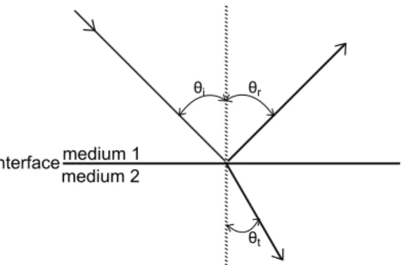
1.3 Transmission and reflection of an acoustic wave on a planar interface
between two media with different acoustic impedances (Z1 for medium1
and Z2 for medium2, Z1 6= Z2); ✓i - angle of incidence and ✓r - angle
of reflection, where ✓i = ✓r; ✓t-different, because the speed of sound is
different in the medium2. . . 7
1.4 The difference between reflection and scattering phenomena. . . 8
1.5 Principle of electronic sweeping with (a) linear array, (b) convex array, and (c) phased array. . . 10 1.6 Ultrasound imaging modalities: (a) conventional and (b) plane-wave
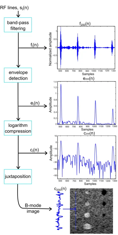
imaging. . . 12 1.7 General ultrasound scanning process. . . 13 1.8 Reconstruction of B-mode image from RF signals. Intermediate data is
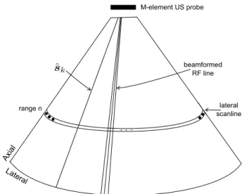
illustrated in the right side of the figure. . . 15 1.9 The spatial coordinate system for illustrating the axial and lateral
resolu-tion configuraresolu-tion of an 1-D ultrasound transducer array. The transducer is divided into elements in the lateral direction. The transmitted US wave propagates in the axial direction. . . 16 2.1 Spatial 2D configuration. The US probe contains M active elements
with the central element is illustrated in blue. The distance from the i-th element to the focal point is ri. The distance from the central element to
the focal point is rc. The delay that is applied to the signal emitted by
the i-th element is ri. In (2.4), the pressure denoted p0(x, y, z, t)refers
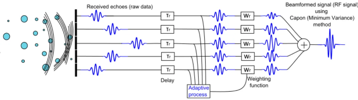
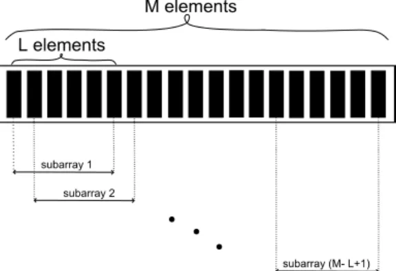
to the one corresponding to the central element, highlighted by blue. . . 20 2.2 The main US imaging elements to model beamforming. . . 21 2.3 Principle of delay-and-sum (DAS) beamformer for (a) emit and (b) receive. 22 2.4 Principle of Capon (Minimum Variance) beamforming in reception. . . . 25 2.5 Subbarray division. The M elements of the array are divided into
over-lapping subarrays of length L. Then, the spatial covariance matrices of
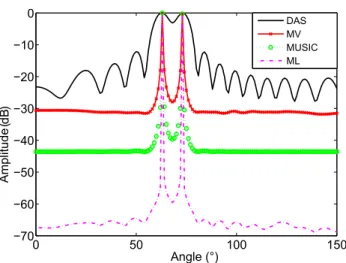
2.6 Comparison between (a) DAS, (b) DAS+CF, (c) MV, and (d) MV+CF. For simulations, an US probe of M = 64 active elements was used. Subarray-averaging method was applied to MV with subarrays of size L = 32. In this case, no temporal averaging was used, so K = 0. . . 29 2.7 Comparison of the lateral profiles at (a) 50 mm and 70 mm from Fig. 2.6. 30 2.8 Comparison between DAS, MV, MUSIC, and ML beamformers
perfor-mance to localize two sources (scatterers) in the medium. . . 32 2.9 Phase shift compensation of the focused raw channel data. . . 34 2.10 Simulated cyst phantom and point reflectors, using an 64-element,
3-MHz phased array. (a) DAS, (b) MV (L=32, T=10), (c) multi-beam Capon (L=32), (d) IAA. At depth 50 mm there are two point reflectors horizontally aligned, with a distance of 1 mm between them. . . 37 2.11 Lateral profiles at 50 mm of the beamformed images in Fig. 2.10. . . 38 3.1 (a) DAS, (b) MV, (c) USBIC, and (d) M-USBIC BF results of 14 sparsely
located reflectors. . . 54 3.2 Lateral variations of the images from the Fig. 3.1 at (a) depth 50 mm
and (b) 70 mm. . . 55
3.3 Results of (a) DAS, (b) MV, (c) USBIC with = 10, and = 0, (d)
M-USBIC with = 70 and = 0, (e) USBIC with = 10, = 0.5, and (f) M-USBIC with = 70 and = 0.7, (g) USBIC with = 10, and (h)
M-USBIC with = 70 on a simulated medium using the phased array
imaging technique. The image quality metrics: CR, CNR, and SNR are given in the Table 3.2. . . 56 3.4 Lateral profiles of the images from the Fig. 3.3. (a) The lateral profile
at the axial depth of 40 mm, that intersects the anechoic cyst; (b) The lateral profile at the axial depth of 70 mm, that intersects the hyperchoic cyst. The lateral profiles were drawn considering USBIC with = 10 and
= 0.5(Fig. 3.3(e)), and M-USBIC with = 70 and = 0.7 (Fig. 3.3(f)). 59
3.5 Values of BIC versus K for USBIC with = 10 and = 0 (Fig. 3.3(c)) and M-USBIC with = 70 and = 0 (Fig. 3.3(d)). . . 59
3.6 Results of (a) DAS, (b) MV, (c) USBIC with = 50, and = 0, (d) M-USBIC with = 25 and = 0, (e) USBIC with = 50, and = 0.5, and (f) M-USBIC with = 25 and = 0.5 on a simulated cardiac apical view image. The image quality metrics: CR, CNR, and SNR are given in the Table 3.3. In (a) we marked the regions used for the calculation of CR, CNR, and SNR. . . 61 3.7 The variation of the CNR and SNR versus the parameters and when
USBIC BF method ((a) and (b)), and M-USBIC BF method ((c) and (d)) are applied to the cardiac view simulation detailed in the Section 3.3.3 63
3.8 Results of (a) DAS, (b) MV, (c) USBIC with = 1, and = 0, (d)
M-USBIC with = 5 and = 0, (e) USBIC with = 10, and = 0.7, and (f) M-USBIC with = 5 and = 0.7 on recorded experimental data. The image quality metrics: CR, CNR and SNR are given in the Table 3.4. In (a) we marked the regions used for the calculation of CR, CNR and SNR. . . 65 3.9 Lateral profiles of the images from the Fig. 3.8. (a) The lateral profile at
the axial depth of 28 mm, that intersects the point reflectors. The red arrows correspond to the point-like reflectors indicated in the Fig. 3.8(a) by red arrows. (b) The lateral profile at the axial depth of 40 mm, that intersects the massive cyst. We considered the case of USBIC with
= 10 and = 0.7 (Fig. 3.8(e)), and of M-USBIC with = 5 and
= 0.7(Fig. 3.8(f)). . . 66 4.1 The elements used to form the proposed model. . . 71 4.2 (a) DAS, (b) MV, (c) multi-beam Capon, (d) IAA, (e) BP, and (f) LS
BF results of the simulation of individual point scatterers. . . 83 4.3 Lateral profiles at 65 mm depth of the point reflectors represented in
Fig. 4.2. . . 84 4.4 (a) DAS, (b) MV, (c) BP, (d) LS, (e) EN ( = 0.8), and (f) EN ( = 0.2)
BF results of a sparse medium. . . 85 4.5 Lateral profiles of Fig. 4.4 at depth 45 mm. . . 86 4.6 (a) DAS, (b) MV, (c) multi-beam Capon, (d) IAA, (e) BP, and (f) LS
4.7 Lateral profiles at 80 mm depth of the cyst phantom represented in Fig. 4.2. 88
4.8 The variation of (a) CNR and (b) SNR versus when BP method was
applied to the hypoechoic cyst simulation. . . 89 4.9 (a) DAS, (b) MV, (c) multi-beam Capon, (d) IAA, (e) BP, and (f) LS
BF results of the ultrarealistic simulation of a cardiac image. . . 90 4.10 (a) DAS, (b) MV, (c) multi-beam Capon, (d) IAA, (e) BP, and (f) LS
BF results of experimental carotid data. . . 92 4.11 (a) DAS, (b) BP, (c) LS, and (d) EN ( = 0.8) BF results of healthy
thyroid in vivo data. . . 95 4.12 (a) DAS, (b) BP, (c) LS, and (d) EN ( = 0.8) BF results of in vivo
thyroid data with tumor. . . 96 5.1 Main elements used to describe the proposed BF model. . . 101 5.2 Results of (a) DAS, (b) MV, (c) LS (Tikhonov), and (d) ↵ stable BF
methods on simulated data with point reflectors and an anechoic cyst structure. The image quality metrics: CR, CNR, and FWHM are given in the Table 5.1. . . 107 5.3 Lateral profiles at 50 mm of the DAS, MV, LS, and ↵-stable BF methods
in Fig. 5.2. . . 107 5.4 The value of ↵ versus the axial distance in Fig. 5.2. . . 108 5.5 Results of (a) DAS, (b) LS, and (c) ↵ stable BF methods on in vivo
data of thyroid with malignant tumor (highlighted by the black arrow). The image quality metrics: CR and CNR are given in the Table 5.2. . . 109 A.1 (a) DAS - simulation (resolution), (b) BP - simulation (resolution), (c)
DAS - experimental (resolution), (d) BP - experimental (resolution), (e) DAS simulation (contrast), (f) BP simulation (contrast), (g) DAS -experimental (contrast), (h) BP - -experimental (contrast). . . 116
1.1 Speed of ultrasound c, specific acoustic impedance Z, and attenuation
coefficients µ (at 1-MHz) for some selected materials [(IAEA), 2014]. . . 6
2.1 CR, CNR, and SNR values for beamformed images in Fig. 2.10 . . . 38 3.1 Parameters of simulated and experimental images . . . 51 3.2 CR, CNR and SNR values of the beamformed images using the simulated
point reflectors and cyst data medium, Fig. 3.3 . . . 58 3.3 CR, CNR and SNR values of the beamformed images using the simulated
cardiac apical view medium, Fig. 3.6 . . . 60 3.4 CR, CNR and SNR values of the beamformed images by using the recorded
experimental data, Fig. 3.8 . . . 66 3.5 Computational time required to beamform the images in the Fig. 3.1 and
Fig. 3.8 . . . 67 4.1 Parameters of simulated and experimental images . . . 78 4.2 CNR, SNR, and RG values for the simulated phantom in Fig. 4.6 . . . . 86 4.3 CNR, SNR, and RG values for the simulated US cardiac beamformed
images in Fig. 4.9 . . . 91 4.4 CNR, SNR, RG, and computational time values for the experimental
4.5 CR, CNR, and SNR values for the in vivo healthy thyroid beamformed images in Fig. 4.11 . . . 95 4.6 CNR, SNR, and RG values for the in vivo thyroidal beamformed images
from Fig. 4.12 . . . 96 5.1 CR, CNR, and FWHM values for simulated data beamformed images in
Fig. 5.2 . . . 106 5.2 CR and CNR values for the in vivo thyroid beamformed images in Fig. 5.5 109 A.1 The characteristics of the L11-4v probe and of the transmit pulse . . . . 115 A.2 Mean resolution scores (axial & lateral) and contrast scores (dB) in Fig.
2D Two-dimensional
3D Three-dimensional
A4C Apical 4 Chambers
ADM alternating direction method
BF Beamforming
BIC Bayesian Information Criteria
BP Basis Pursuit
BS-Capon Beamspace Capon
CNR Contrast-to-noise ratio
CR Contrast ratio
CS Compressive Sensing
DAS Delay-and-Sum
DFT Discrete Fourier Transform
DL Diagonal loading
EN Elastic-net
ES-Capon Element-space Capon
Field II Ultrasound simulator software
package
FWHM Full width at half maximum
IAA Iterative Adaptive Approach
LASSO Least Absolute Shrinkage and
Selection Operator
LCMV Linear Constrained Minimum
Variance
LS Least Squares
LV Left Ventricle
M-USBIC Beamformer based on MV
RF image
ML Maximum Likelihood
MUSIC MUltiple SIgnal Classification
MV Minimum Variance
OMP Orthogonal Matching Pursuit
RG Resolution Gain RV Right Ventricle S↵S Symmetric ↵-stable SINR Signal-to-interference-plus-noise ratio SNR Signal-to-noise ratio
TGC Time Gain Compensation
US Ultrasound
USBIC Beamformer based on DAS RF
image
YALL1 Software package to solve
Introduction
L’imagerie ultrasonore(US) est l’une des techniques d’imagerie médicale qui
con-nait les développements les plus rapides notamment grâce à ses propriétés non invasives, ses méthodes d’acquisition rapides, et son coût modéré. L’imagerie cardiaque, abdom-inale, fœtale, ou mammaire sont quelques-unes des applications où elle est largement utilisée comme outil de diagnostic.
En imagerie US classique, des ondes acoustiques sont transmises à une région d’intérêt du corps humain. Les signaux d’écho rétrodiffusés, également appelés données brutes, sont ensuite traités pour créer des lignes radiofréquences (RF). La formation de voies (FV) joue un rôle clé dans l’obtention des images US, car elle influence la résolution et le contraste de l’image finale. La méthode standard en formation de voies dite DAS ("delay-and-sum") consiste à retarder et à pondérer les échos réfléchis avant de les moyenner. Les méthodes de FV existantes utilisent des poids fixes ou adaptatifs pour le moyennage. L’objectif de ce travail est de modéliser la formation de voies comme un problème inverse liant les données brutes aux signaux RF. Le modèle de formation de voies proposé ici améliore le contraste et la résolution spatiale des images échographiques par rapport aux techniques de FV existants.
Le premier chapitre de cette thèse donne le cadre théorique de l’imagerie US. En premier lieu, nous presentons les caractéristiques des signaux US, et fournissons une analyse de la propagation des ondes. Ensuite, nous présentons l’imagerie médicale US, et la manière dont les images sont affichées. Enfin, la formation de voies est introduite et les principales méthodes de formation de voies sont brièvement décrites, ainsi que leurs limites.
Le second chapitre présente l’état de l’art des méthodes de formation de voies ex-istantes en imagerie médicale ultrasonore. Nous passons brièvement en revue les tech-niques de formation de voies les plus courantes, en commençant par la méthode dite DAS, puis les techniques émergentes les plus connues de formation de voies adaptatives, en mettant l’accent sur la méthode à variance minimale (MV) ainsi que ses variantes.
présentée.
Le troisième chapitre propose l’utilisation des signaux qui exploitent une représen-tation parcimonieuse de l’image US. Notre méthode est basée sur la création de méth-odes de formations de voies originales en deux dimensions pour l’imagerie US. Les approches proposées détectent les réflecteurs forts du milieu à imager sur la base de critères bayésiens bien connus et utilisés dans la modélisation statistique. En outre, ils permettent une sélection du niveau de bruit dans l’image finale BF.
Dans le quatrième chapitre, nous proposons une nouvelle façon d’aborder la forma-tion de voies en imagerie US, en la formulant comme un problème inverse linéaire liant les échos réfléchis au signal final. Notre approche présente deux avantages majeurs : i) sa flexibilité dans le choix des hypothèses statistiques sur le signal avant la formation de voies (les statistiques Laplaciennes et Gaussiennes) et ii) sa robustesse à un nombre réduit d’impulsions d’émissions. Le cadre proposé est souple et permet de trouver un compromis entre la suppression du bruit et la netteté de l’image résultante. Nous il-lustrons la performance de notre approche à la fois sur des données simulées et sur des données in vivo de carotide et de thyroïde.
Dans le cinquième chapitre, nous présentons une nouvelle méthode de formation de voies pour l’imagerie médicale US basée sur l’utilisation de caractéristiques statistiques des signaux supposées ↵-stable. Bien que le traitement du signal US se soit largement appuyé pendant de nombreuses années sur l’hypothèse Gaussienne, il a été montré que les échos RF peuvent être modélisés avec plus de précision par une loi statistique à "queue lourde". Par exemple, les propriétés statistiques des signaux RF peuvent être considérés, d’après le théorème central limite generalisé, ↵-stables. La principale contribution de ce chapitre est l’utilisation des propriétés non-gaussiennes des signaux RF dans le processus de formation de voies. Il s’agit de la première tentative considérant spécifiquement une distribution ↵-stable, pour la formation de voies en imagerie US.
Principe de l’imagerie ultrasonore Sonde ultrasonore Diffuseurs dans le milieu Propagation de l'onde dans le milieu Echos réfléchis Données brutes Excitation (a) (b) (c) Ondes ultrasonores émises dans le milieu
Figure 1: Principe de l’imagerie US : (a) une impulsion électrique (excitation) est trans-mise au transducteur piézoélectrique qui la transforme en une onde US; (b) l’onde se propage et interagit avec le milieu; (c) les ondes réfléchies reçues par le transducteur sont converties en signaux électriques (données brutes).
Le principe de l’imagerie ultrasonore (US) est illustré à la Fig. 1. Il repose sur l’interaction entre les ondes US et le milieu qui contient les diffuseurs. Ces dernières sont produites à l’aide de matériaux piézoélectriques constituant la sonde US et sont émises en direction du milieu (Fig. 1(a)). Au cours de leur propagation à travers le milieu, des phénomènes de réflexion et de transmission se produisent à l’interface de milieux ayant différentes impédances acoustiques. De plus, l’amplitude de l’onde US est atténuée en raison des phénomènes d’absorption et de diffusion [Kuttruff, 1991].
Actuellement, la grande majorité des sondes US sont constituées de plusieurs élé-ments disposés linéairement ou sectoriellement. Ils permettent à la fois l’émission des ondes US et la réception des échos réfléchis par le milieu (Fig. 1(b)). Ces échos, trans-formés en signaux électriques puis numérisés, représentent les données brutes acquises par le système US (Fig. 1(c)). Afin d’améliorer la résolution spatiale, le rapport signal
appliquées aux données US brutes pour produire des signaux radiofréquences (RF). Visualisation des images ultrasonores
Pour des raisons de lisibilité, les images RF sont finalement converties en images en mode B (brillance), à l’aide de post-traitements classiques tels que le filtrage passe-bande, la détection d’enveloppe et la compression logarithmique. Afin de pouvoir comparer les résultats proposés dans cette thèse avec les techniques de formations de voies existantes, nous utiliserons les mesures les plus courantes de qualité d’image : le rapport de con-traste (RC) [Xu et al., 2014a], le rapport concon-traste sur bruit (RCB) [Rindal et al., 2014], et le rapport signal sur bruit (RSB) [Jensen and Austeng, 2014].
Formation de voies en imagerie ultrasonore
Les techniques de formation de voies jouent un rôle majeur dans la qualité des im-ages US [Van Veen and Buckley, 1988]. La méthode couramment employée en imagerie US utilise les opérations classiques de retard et somme dite DAS (delay-and-sum) [Thomenius, 1996]. Avec cette méthode, les donées brutes reçues par les éléments de la sonde sont d’abord focalisées afin de compenser les retards dus aux différences de temps de propagation, avant d’être sommées en les pondérant par des coefficients. Ces coefficients forment la fenêtre d’apodisation en réception. Malgré son avantage lié es-sentiellement à sa rapidité, la méthode par retard et somme ne permet pas d’obtenir une résolution spatiale et un contraste optimal. Afin d’améliorer la qualité des images RF, de nombreux travaux existant proposent d’adapter les fenêtres d’apodisation aux données, ou autrement dit de les estimer à partir des données brutes. L’une des méth-odes les plus utilisées est celle du filtre de Capon [Capon, 1969]. Son rôle est d’appliquer une fenêtre d’apodisation optimale afin d’estimer la forme d’onde du signal désiré aussi précisément que possible, tout en rejetant les signaux indésirables. D’autres exemples de formeurs de faisceaux adaptatifs sont les techniques MUSIC [Schmidt, 1981] et Max-imum Likelihood (ML)([Krim and Viberg, 1996, Stoica and Sharman, 1990]).
La formation de voies (FV) permet d’amplifier les signaux réfléchis depuis des posi-tions connues, tout en atténuant les signaux provenant de posiposi-tions indésirables. Ceci est classiquement réalisé en retardant et en appliquant des poids spécifiques aux sig-naux réfléchis. Les formeurs de voies peuvent être soit indépendants des données (fixes), dépendants des données (adaptatifs), en fonction du calcul des poids appliqués aux sig-naux réfléchis.
Formation de voies non-adaptative
La formation de voies par retard et somme, dite DAS (delay-and-sum), sélectionne les
poids wDAS indépendamment des données :
wDAS =
1
M, (1)
où 1 est un vecteur colonne de longueur M constitué de "un" car les données brutes ont été focalisées à l’aide de retards.
Nous considérons ci-après le schéma d’acquisition classique où une série de K voies focalisées est transmise avec M éléments. Les K voies focalisées sont transmises avec des angles d’incidence différents ✓k, k = 1,· · · , K. L’image finale RF US est un ensemble de
lignes RF. Chacune d’elle étant le résultat de la formation de voies à partir des signaux RF bruts provenant d’une émission dans la direction ✓k, k 2 {1, . . . , K}, en utilisant M
éléments du transducteur. La formation de voies classique par retard et somme peut être exprimée comme suit :
ˆ
sk= wHyk, (2)
où yk 2 CM⇥N sont les données brutes compensées en temps reçues par le m-ième
élément de la sonde US, et correspondant à l’émission dans la direction ✓k, et w est le
vecteur des poids du formateur de voies et de taille M ⇥ 1. Formation de voies adaptative
Bien que la formation de voies par retard et somme utilise des poids fixes, le but de la formation de voies à variance minimum (MV) est d’appliquer un ensemble de poids dépendant des données (d’où le nom adaptatif). Ceci afin d’estimer la forme d’onde
L’expression des poids utilisés par la MV est : wM V = Rk11 1TR 1 k 1 , (3)
où Rk est la matrice de covariance. Il est à noter que dans la pratique, une simple
estimation de la matrice de covariance peut être faite. Celle-ci peut être mal condition-née et ainsi engendrer des résultats moins bons que ceux de la méthode par retard et somme.
Afin d’améliorer la robustesse de la formation de voies MV, différentes techniques ont été proposées dans la littérature : sous-matrice d’étalement (pour décorréler des signaux cohérents), moyenne temporelle (pour conserver des statistiques de speckle), rehaussement de la diagonale (pour améliorer la robustesse de l’inversion de la matrice de covariance), pondération par facteur de cohérence (pour augmenter la résolution et le contraste de l’image obtenue après l’application de la méthode MV), ou encore utilisation de sous-bandes de fréquences.
La formation de voies dans d’autres domaines
Un problème particulier résolu par la formation de voie est la localisation de sources (en particulier sur la direction d’arrivée). Le problème inverse sur lequel est basé le problème de la localisation des sources peut être exprimé comme suit :
y = T (x) + n, (4)
où x 2 X est inconnu, y 2 Y est le vecteur des mesures (observations), X, sont des espaces de Hilbert, et n est un bruit blanc gaussien. Le but est de trouver x à partir de y connaissant la transformation T . La solution de (4) est généralement présentée comme : ˆ x = argmin x (ky T (x)k 2 2+ P (x)), (5)
où le premier terme, ky T (x)k2
2 est le terme d’attache aux données, et P (x) est une
fonction traduisant les connaissances à priori sur x. Ce terme est aussi appelé le terme de régularisation. Dans cette thèse, nous avons modélisé le problème de FV en imagerie médicale US en utilisant le problème inverse formulé dans (4) et nous avons appliqué différentes techniques de régularisation dans le but de résoudre (5).
Dans ce chapitre, nous proposons une méthode de formation de voies qui exploite une représentation parcimonieuse des images RF. Une détection automatique des forts échos susceptibles de représenter les frontières entre les organes ou des structures hy-peréchogènes a été effectuée en réalisant un compromis entre la parcimonie spatiale de ces structures et la forme des données brutes. L’image ainsi obtenue est par la suite combinée linéairement avec une image classiquement formée, afin de garder le speckle habituel des images. Nous avons montré à travers des résultats de simulations réalistes et un résultat expérimental sur fantôme (matériau de test) que la méthode proposée améliore le contraste et le rapport signal sur bruit comparé à des approches de formation de voies classiques.
Formation de voies proposée
La détection est basée sur un compromis entre la parcimonie spatiale des images obtenues et le respect des données brutes. Le modèle parcimonieux de l’image RF considéré s’écrit sous la forme suivante [Tur et al., 2011] :
S(x, n) = P X p=1 aphp(x xp, n np), x = x1,· · · , xM et n = 1, · · · , N, (6) avec n et x les variables spatiales respectivement axiales (dans la direction de propa-gation des ondes) et latérales, S(x, n) la représentation parcimonieuse de l’image RF après formation des voies, (xp, np) avec p = 1 · · · P les positions spatiales des P plus
forts diffuseurs du milieu imagé. Les ap représentent les amplitudes des diffuseurs et
hp(x, n)sont les formes d’ondes réfléchies par chaque diffuseur.
Dans notre modèle, les positions, les amplitudes et les réponses produites par chaque diffuseur sont considérées inconnues et seront estimées. La parcimonie est liée au fait que le nombre de diffuseurs forts K est très faible dans la grille spatiale 2D des positions considérées initialement par le formeurs de voies. Notre méthode est constituée de deux étapes. La première détecte un fort diffuseur potentiel en se basant sur l’image RF for-mée par l’approche par retard et somme ou par variance minimum. La deuxième étape valide ce choix en évaluant l’évolution d’une fonction de coût faisant appel aux données
de coût dont l’objectif est de trouver un compromis entre un faible nombre d’échos forts et le respect des données brutes. Cette fonction, inspirée du critère d’information Bayesien [Konishi and Kitagawa, 2008] est adaptée à l’imagerie US.
Expériences
Les approches proposées, nommées USBIC (basées sur le retard et la somme) et M-USBIC (basé sur la variance minimum), ont été évaluées sur trois différents exemples simulés en utilisant le programme de simulation Field II et des acquisitions sur des fantômes US. Le premier milieu simulé est basé sur une hypothèse de réflecteurs parci-monieux. Le second est basé sur des données simulées à partir d’un milieu contenant des réflecteurs parcimonieux, un kyste, et du speckle, en utilisant une sonde multi-éléments. Le troisième exemple représente la simulation d’une image cardiaque en vue apicale 4-chambre (A4C), comme suggérée dans [Alessandrini et al., 2012]. Les données expérimentales ont été acquises avec une plateforme de recherche Ultrasonix MDP. Résultats
La première simulation consiste en un milieu contenant 14 réflecteurs parcimonieux, alignés latéralement à 2 mm et 2 mm. Le milieu ne contient pas du speckle. Dans la simulation, nous avons évalué le potentiel des méthodes proposées à détecter avec précision les réflecteurs forts dans des milieux parcimonieux. Les résultats montrent que l’ensemble des 14 réflecteurs positionnés parcimonieusement est détecté aux positions correctes. La deuxième simulation contient des réflecteurs forts et un kyste dans un milieu avec du speckle. Le principal avantage de notre méthode est d’améliorer le contraste pour des structures hyperéchogènes. Cependant, en ajoutant le speckle sur des images finales, malgré une réduction du contraste, nous parvenons à maintenir un contraste voisin de celui obtenu par des techniques de formation de voies existantes. Troisièmement, les résultats de formation de voies sur une vue A4C simulée montrent que les méthodes proposées améliorent le contraste des structures du ventricule, tout en conservant leurs formes. Enfin, en les appliquant sur des données expérimentales, nous avons montré que la méthode proposée offre un meilleur compromis entre le contraste et la préservation du speckle, comparée aux formateurs de voies par retard et somme et à variance minimum.
Dans ce chapitre, nous proposons d’effectuer la formation de voies en imagerie ul-trasonore par un problème inverse régularisé basé sur un modèle linéaire reliant les échos réfléchis au signal final recherché. La contribution majeure de ce chapitre est l’amélioration des techniques de formation de voies existantes en combinant le mod-èle direct proposé formulé suivant la direction latérale des images avec une approche d’inversion régularisée. De plus, la méthode proposée permet de réduire fortement le nombre d’émissions US requises.
En premier lieu, les statistiques laplaciennes (`1) et gaussiennes (`2), deux des
régu-larisations les plus courantes dans de tels problèmes d’imageries, seront considérées ici ([Chen et al., 1998, Tikhonov, 1963]). En second lieu, nous avons également appliqué
à notre cadre, une méthode de régularisation complexe combinant `1 et `2, appelée
régularisation « elastic-net » [Zou and Hastie, 2005]. En outre, notre méthode ouvre de nouvelles perspectives pour les termes de régularisation plus complexes (par exem-ple, [Chen et al., 2016a, Michailovich and Rathi, 2015]) pour améliorer davantage les résultats.
Formation de voies proposée
La méthode proposée est appliquée séquentiellement de la même manière à chaque échantillon (profondeur). Pour chaque profondeur n, nous souhaitons estimer le signal correspondant à un réflecteur en fonction de son emplacement, qui contiendra des pics dominants à la position des réflecteurs. Nous rappelons ici que nous utilisons le même mode d’acquisition que celui décrit dans le Chapitre 2, où une série de K voies focalisées sont transmises avec M éléments, avec des angles d’incidence différents ✓k, k = 1,· · · , K.
Comme il s’agit de plusieurs directions, pour réduire la complexité élevée, nous pro-posons d’utiliser les données formées par la méthode par retard et somme au lieu de les former à partir des données brutes. Ensuite, nous utilisons un outil couramment util-isé dans les approches de localisation des sources permettant de réduire la complexité de calcul [Fuchs, 1996, Tian and Van Trees, 2001]. Plus précisément, pour chaque pro-fondeur n, nous projetons les données obtenues lors de la formation de voies par retard
ABS.
Notre modèle est formulé ainsi :
z[n] = (AHBSA)x[n] + DHg[n], (7)
où z[n] 2 CP⇥1est le vecteur transformé formé par l’échantillonnage des lignes latérales
formées par la methode par retard et somme sur une grille de P positions, D de taille K⇥P est une matrice de décimation, x[n] de taille K ⇥1 est le profil latéral à estimer à
la profundeur n, et A respectivement ABS sont les matrices de projection des capteurs
vers les reflecteurs dans le milieu et des reflecteurs vers les capteurs.
Une façon d’inverser le problème est d’utiliser des techniques standards de régularisa-tion. En considérant que le signal x[n] suit les statistiques laplaciennes, la minimisation de la fonction de coût s’écrit :
x[n] = argmin
x[n]
(||z[n] (AHBSA)x[n]||22+ ||x[n]||1), (8)
où ||·||1désigne la norme `1. Nous avons utilisé l’outil d’optimisation YALL 1 [Zhang, 2009]
pour résoudre (8). Expériences
Les approches proposées, appelées de façon générique dans ce chapitre : « Base Pursuit beamforming » (BP BF), « Least Squares beamforming » (LS BF), et « Elastic-Net beamforming » (EN BF), ont été évaluées en utilisant des données simulées et des données expérimentales in vivo de la carotide et de la thyroïde.
Résultats
Nous présentons les résultats de formation de voies sur des données de la thyroïde avec une tumeur. Nous pouvons observer que contrairement à l’image DAS, où la tumeur est difficile à distinguer (voir Fig. 2(a)), les méthodes proposées (BP, LS, et EN) améliorent la visualisation des principales structures, et renforcent les bords de la tumeur (voir Fig. 2(b)-(d)).
Dist ance axia −50 0 50 30 40 50 60 70 −50 0 50 (a) (b) −50 0 50 (c) [dB] −50 0 50 −60 −50 −40 −30 (d) Distance laterale (mm)
Figure 2: Les résultats de la formation de voies (a) par retard et somme, (b) BP, (c) LS, et (d) EN ( = 0.8) sur des données in vivo de la thyroïde avec une tumeur.
Conclusions
Contrairement aux techniques existantes qui utilisent des poids adaptatifs, nous avons regularisé notre problème inverse de formation de voies en utilisant des hypothèses statistiques laplaciennes, gaussiennes, et « elastic-net ». La FV à base de régularisation proposée permet de réduire fortement le nombre de transmissions US (par un facteur cinq dans nos exemples), tout en améliorant la qualité des images formées en termes de résolution et de contraste par rapport aux formeurs de voies existants.
utilisant une loi stable
Dans ce chapitre, nous présentons une nouvelle méthode de formation de voies basée sur la caractérisation statistique des signaux par des distributions ↵-stable. La principale contribution présentée dans ce chapitre est l’utilisation des propriétés non gaussiennes des signaux RF dans le processus de formation de voies (voir par exem-ple [Pereyra and Batatia, 2012, Alessandrini et al., 2011, Zhao et al., 2016b]). A notre connaissance, ceci est la première tentative de considérer spécifiquement une distribu-tion ↵-stable pendant la formadistribu-tion de voies en imagerie US.
Formation de voies proposée
Le modèle linéaire direct présenté dans le Chapitre 4 est ici inversé en utilisant une régu-larisation par pseudo-norme plus générale `p, avec p automatiquement lié au paramètre
↵ estimé à partir des données brutes [Achim et al., 2015]. Notre solution de FV est
basée sur l’hypothèse d’une distribution ↵-stable des signaux US. La loi stable est une généralisation de la distribution gaussienne (pour ↵ = 2, la distribution stable est ré-duite à la distribution gaussienne) [Shao and Nikias, 1993].
Dans [Achim et al., 2015], il a été montré que la régularisation par norme `pest bien
adaptée pour reconstruire des signaux suivant une distribution ↵-stable symétrique (S↵S). En outre, il a été démontré que le choix optimal pour le paramètre p est plus petit, mais aussi proche que possible de ↵ [Achim et al., 2015], généralement p =
↵ 0, 01. Selon le degré de parcimonie du milieu, la valeur de p, directement liée
à ↵ estimée à partir de y (soit p = ↵ 0, 01) peut prendre des valeurs plus petites
que 1. Dans ce cas, la fonction de coût à minimiser devient non convexe. Plusieurs solutions pour résoudre ces problèmes non convexes existent dans la littérature. Dans ce travail, nous avons utilisé l’algorithme d’optimisation semi-quadratique proposé dans [Cetin and Karl, 2001].
Expériences
Afin d’évaluer la méthode de FV proposée (notée FV ↵-stable), nous avons utilisé à la fois des données simulées et in vivo. Les données simulées contiennent 3 diffuseurs situés à 50 mm de profondeur et une structure de kyste anéchoïque de 10 mm de rayon
(d) [dB] −20 0 20 −80 −60 −40 (c) Distance laterale (mm)−20 0 20 (a) (b) Dist ance axia le −20 0 20 80 100 120 −20 0 20
Figure 3: Les résultats de la formation de voies (a) par retard et somme, (b) à variance minimum (c) LS, et (d) ↵-stable sur des données simulées contenant 3 réflecteurs et un kyste hypoéchogène.
situé à 80 mm de profondeur, noyés dans du speckle. Les émissions correspondaient à 52 ondes planes (pour la méthode proposée) et à 260 ondes planes (pour les méthodes de formation de voies par retard et somme et à variance minimum) transmises avec des angles compris entre -30 et 30 . Les données in vivo représentent la glande thyroïde d’un sujet atteint d’une tumeur maligne. L’acquisition a été réalisée avec un système clinique d’échographie Sonoline Elegra modifié à des fins de recherche, et équipé d’un transducteur en réseau linéaire Siemens Medical Systems 7.5L40 P / N 5260281-L0850 émettant des séries d’ondes focalisées.
Résultats
Nous présentons ici les résultats de FV des données simulées contenant 3 réflecteurs et un kyste hypoéchogène. Nous pouvons observer que la formation de voies par retard et somme (Fig. 3(a)) n’est pas en mesure de résoudre la dimension du kyste circu-laire. En effet, le kyste apparaît plus étroit que sa dimension d’origine, en raison de la faible résolution fournie par la formation de voies par retard et somme. La méthode à variance minimum (Fig. 2(b)) et la LS (Fig. 2(c)) fournissent de meilleurs résultats, à savoir une dimension du kyste plus proche de sa dimension réelle. Toutefois, lorsque nous utilisons une formation de voies ↵-stable (Fig. 2(d)), nous obtenons de meilleurs résultats en termes de résolution spatiale, de contraste , par rapport aux méthodes par retard et somme, à variance minimum et LS. Nous notons que les méthodes par retard et somme et à variance minimum ont utilisé des données brutes obtenues avec cinq fois plus d’émissions US que notre méthode (i.e 260 ondes planes). Grâce à cet exemple,
d’émissions. Conclusions
Dans ce chapitre, nous avons proposé une nouvelle méthode de formation de voies en généralisant le modèle proposé précédemment (présentée dans le Chapitre 4). Notre
méthode utilise une régularisation par pseudo-norme `p pour résoudre notre problème
inverse. De plus, p est calculé automatiquement en le reliant aux statistiques ↵-stables des images US. Ainsi, notre méthode, contrairement aux approches à variance minimale, ne nécessite qu’un seul réglage des paramètres. Elle pourrait également être d’un intérêt dans d’autres domaines d’application tels que l’estimation de la direction d’arrivée. Les travaux futurs porteront sur l’évaluation d’autres stratégies d’acquisition (par exemple, émissions d’ultrasons dans des directions aléatoires) ou encore sur la prise en compte des termes de régularisation communs pour la reconstruction conjointe de plusieurs lignes latérales.
Ultrasound (US) imagingis one of the most fast-developing medical imaging tech-niques, allowing non-invasive and ultra-high frame rate procedures at reduced costs. Cardiac, abdominal, fetal, and breast imaging are some of the applications where it is extensively used as diagnostic tool.
In a classical US scanning process, short acoustic pulses are transmitted through the region-of-interest of the human body. The backscattered echo signals, also called raw channel data, are then processed for creating radiofrequency (RF) beamformed lines. Beamforming (BF) plays a key role in US image formation, influencing the resolution and the contrast of final image. The standard way of BF is to delay and weight the reflected echoes before averaging them. Most of the existing BF methods are using fixed (data-independent) or adaptive (data-depended) weights. The focus of these methods is to calculate the weights applied to the reflected echoes, such that only the signals of interest are preserved. Data-independent BF methods provide results with low resolution and contrast. The results are improved by data-dependent BF methods. However, their computation complexity is high and they are not adequate for real-time applications.
The objective of this work is to model BF as an inverse problem, relating the raw channel data to the signals to be recovered. The proposed BF framework improves the contrast and the spatial resolution of the US images, compared with the existing BF methods.
The first chapter of the thesis provides the background of ultrasound imaging. Firstly, it illustrates the characteristics of US signals, and analyzes the propagating waves. Secondly, beamforming technique is introduced. Then, the main source localiza-tion methods are briefly described, together with their limitalocaliza-tions. Thirdly, we present the medical US imaging, and the way the US images are displayed.
medical US imaging. We briefly review the most common beamforming techniques, starting with the standard delay-and-sum (DAS) BF method and emerging to the most known adaptive BF techniques, with focus on the minimum variance (MV) BF and its improvements. A detailed comparison between the presented BF methods is presented. The third chapter investigates the use of sparse priors in creating original two-dimensional beamforming methods for ultrasound imaging. The proposed approaches detect the strong reflectors from the scanned medium based on the well-known Bayesian Information Criteria used in statistical modeling. Moreover, they allow a parametric selection of the level of speckle in the final beamformed image.
In the fourth chapter, we propose a new way of addressing the BF in US imaging, by formulating it as a linear inverse problem relating the reflected echoes to the signal to be recovered. Our approach presents two major advantages: i) its flexibility in the choice of statistical assumptions on the signal to be beamformed (Laplacian and Gaussian statistics are tested herein) and ii) its robustness to a reduced number of pulse emissions. The proposed framework is flexible and allows for choosing the right trade-off between noise suppression and sharpness of the resulted image. We illustrate the performance of our approach on both simulated and experimental data, with in vivo examples of carotid and thyroid.
In the fifth chapter, we present a new beamforming method for ultrasound medical imaging based upon the statistical characterization of the ultrasound signals by ↵-stable distributions. In the chapter four we have reformulated BF in US imaging as a linear inverse problem, associating the raw channel data to the RF signals to be recovered. While US signal processing has widely relied for many years on the assumption of Gaussianity it was shown that RF echoes can be more accurately modelled by a power-law shot noise model. For example, the statistical properties of the RF signals were related, based on the generalized central limit theorem, to ↵-stable distributions. The main contribution of this chapter is the use of the non-Gaussianity properties of the RF signals in the beamforming process. This is the first attempt of specifically considering an ↵-stable distribution while beamforming the received echoes in US imaging.
Finally, the sixth chapter discusses the contributions of the thesis and the future works.
Before we discuss about the beamforming process and contributions we proposed, it is necessary to present the main principles of ultrasound imaging. Thus, we start the first chapter of the manuscript by presenting the most important aspects of ultrasound (US) imaging, which are very important for a good understanding of the material presented in this thesis. Firstly, the principle of ultrasound imaging is described, together with the basic physical phenomenon. Then, the techniques for US image visualization, with focus on medical US imaging are presented. Finally, the basics of beamforming (BF) are introduced, and some of the most common BF techniques are described.
1.1 Ultrasound imaging principles
We start this chapter by describing the basic principle of US imaging, including sound propagation and classical scanning methods of the medium.
1.1.1 Principle of ultrasound imaging
Ultrasonic field has been extensively developing since 1970s and it represents approxi-mately 25% of all medical imaging examinations performed in the world at the beginning of 21st century [(IAEA), 2014]. There exist distinct fields of study within ultrasonics, with different applications, as: underwater acoustics, applications for monitoring and control, medical ultrasonics for therapy, diagnosis, surgery, biotechnology, nanotechnol-ogy, and defense. All these domains are in continuous development.
Ultrasound signals are acoustical waves with frequencies in the range 20 kHz to
1 GHz. These waves are produced by electrically exciting a piezoelectric transducer
which is capable of generating and detecting ultrasound energy. Note that the same transducer is used for both transmission and reception of the ultrasound waves in the medium. In function of their frequencies, the acoustic waves can be classified as:
• Infrasounds: f 20 Hz. These sound waves cannot be perceived by human ear. Their main application is monitoring the earthquakes.
• Audible sounds: 20 Hz f 20 kHz. This is the hearing range of frequencies in humans and most of the animals.
Transducer Emitted ultrasound wave Scatterers in the medium Propagation of the wave through the medium
Echoes
Raw channel data Excitation
(a) (b) (c)
Figure 1.1: The principle of ultrasound imaging: (a) an electrical pulse (excitation) is transmitted to the piezoelectric transducer, transforming the pulse into an ultrasound wave; (b) the wave propagates and interacts with the medium; (c) the reflected waves received by the transducer are transformed in electrical signals (raw channel data).
C C C C D D D D distance pressure C D C D C D C D +∆P ∆P
-Figure 1.2: Propagation of a 1D longitudinal wave in homogeneous, loss-less medium. The pressure p(x, t) is alternatively compressed (C) and expanded (D).
• Ultrasounds: 20 kHz f 1 GHz. They contain frequencies higher than the upper audible limit of human hearing. Their main application domains are industry and medicine.
• Hypersounds: f 1 GHz. They are also called ’microwave acoustics’. A
quantitative investigation of such waves can be done using Bragg diffraction [Kuttruff, 1991].
Fig. 1.1 presents the basic principle of ultrasound imaging. Firstly, acoustic waves (vibrations) are generated (Fig. 1.1(a)). The emitted ultrasound waves are propagating and interacting to the medium (Fig. 1.1 (b)). Due to the interaction and due to the inhomogeneities that are present within the medium, some reflected and diffused waves will rise. These echoes propagate back towards the transducer, which will translate them in electrical signals (raw channel data) proportional with the received echoes (Fig. 1.1 (c)).
Until here, we presented the basic principle of ultrasound imaging, without taking into account the properties of sound, their propagation laws, the design of the trans-ducers, or aspects about how we can visualize the signals reflected from the medium. Leaving out the details, the next few sections will present the sound and transducer properties, for a better understating of the principle of interaction between the sound and the particles in the propagating medium. For a more thorough covering of the material presented in this section the reader is referred to [(IAEA), 2014].
1.1.2 Sound propagation in medium
We present here the main properties of the sound and the way it interacts with the medium, by emphasizing the phenomena of propagation, reflection, transmission, scat-tering, absorption, and attenuation.
The tissue is a medium where sounds propagate and where exchange between kinetic and potential energy takes place. In biological tissues and water, we primarily find longitudinal waves. This type of waves is propagated by the tissue particles that are alternatively compressing and decompressing, as illustrated in the Fig. 1.2.
The propagation phenomenon can be described by the wave equation. A wave in homogeneous medium without attenuation, at a position (x, y, z) of the propagating space and at a time t can be described by a second-order differential equation:
r2p 1
c2
@2p(x, y, z, t)
@t2 = 0, (1.1)
where r2 is the Laplacian operator and r2p = @2
@x2p + @ 2
@y2p + @ 2
@z2pand c is the speed
of sound in the medium and has the expression:
c = p1
⇢, (1.2)
where ⇢ is the medium density and [Pa 1] the medium compressibility. The average
speed of sound in the human body is 1540 m/s. It is slowest in air/gasses and fastest in solids. The values of speed of sound in different biological materials are described in Table 1.1.
The other parameters of the Table 1.1 will be introduced later in the manuscript. When the wave propagates in one direction, for example x direction, it is re-ferred to as plane wave. In this case, the propagation equation (1.1) become (e.g., [Angelsen, 2000b, Angelsen, 2000a]):
@2p(x, t) @x2 1 c2 @2p(x, t) @t2 = 0, (1.3)
where p(x, t) represents the pressure that is function of the position x and time t. One solution of (1.3), important for this work, in the case of plane wave equation given by:
Material c(m/s) Z(kg·m 2·sec 1)⇥ 10 4 dB/cm at 1 MHz Air 330 0.0004 12 Water 1480 1.48 0.0022 Fat 1450-1460 1.34-1.38 0.52 Brain 1560 1.55 0.85 Liver 1555-1570 1.65 0.96 Kidney 1560 1.62 1.0 Spleen 1570 1.64 1.0 Blood 1550-1560 1.61-1.65 0.17 Muscle 1550-1600 1.62-1.71 1.2 Lens of eye 1620 1.85 2.0 Skull bone 3360-4080 6.0-7.8 11.3
Table 1.1: Speed of ultrasound c, specific acoustic impedance Z, and attenuation coeffi-cients µ (at 1-MHz) for some selected materials [(IAEA), 2014].
p(x, t) = Aej(!t kx), (1.4)
where A is the amplitude of the propagating signal, !
2⇡ is the frequency, and k = !c is the
wavenumber. The name of plane wave equation is given by the fact that the wavefronts form planes in the 3-D space. Note that (1.4) is defined for one spatial dimension.
Considering that the plane wave in (1.4) propagates through the medium and is reflected, the measured signal at the sensor is defined as:
y(t) = Aej(!t kx). (1.5)
The acoustic properties of the medium are characterized by the acoustic impedance, which can be seen as the opposition to the flow of sound through a surface. The acoustic impedance, Z, similar to the electric impedance, allows the characterization of a medium based on its density, ⇢, and the speed of sound in that medium:
Z = ⇢c. (1.6)
The commonly used unit to quantify the specific acoustic impedance is the rayl, and it is defined as 1[rayl] = 1[kg·m 2·s 1]. The specific acoustic impedance of some
interface
θi θr
θt
medium 1 medium 2
Figure 1.3: Transmission and reflection of an acoustic wave on a planar interface between
two media with different acoustic impedances (Z1for medium1 and Z2for medium2, Z16=
Z2); ✓i- angle of incidence and ✓r- angle of reflection, where ✓i= ✓r; ✓t-different, because
the speed of sound is different in the medium2.
1.1.2.1 Reflection and transmission
During the propagation, sound can travel different types of tissues. In this case, reflec-tion or transmission phenomena may occur which are described in this secreflec-tion.
Through the propagation of the wave in the medium, a portion of the incident energy (Ii) is reflected (Ir), while the second portion is transmitted (It), as illustrated
in Fig. 1.3. The reflection coefficient ↵R is used to measure the reflection between two
adjacent tissues with different impedances, Z1 and Z2:
↵R= Ir Ii = ( Z2 cos ✓t Z1 cos ✓i) 2 ( Z2 cos ✓t + Z1 cos ✓i) 2. (1.7)
The sound wave that is not reflected, will be transmitted into the medium. The transmission coefficient ↵T is expressed as:
↵T =
It
Ii
= 1 ↵R. (1.8)
The equations governing the angles of incidence ✓i, reflection ✓r, and transmission
✓t, are the following:
✓i= ✓r, sin ✓i sin ✓t = c1 c2, (1.9) where c1 and c2 are the sound velocities in the medium 1, respectively medium 2.
interface
Reflection Scattering Scattering
Figure 1.4: The difference between reflection and scattering phenomena.
In the case when ✓i = ✓t = 0, we can rewrite (1.7) depending just on the ratio
between Z1 and Z2: ↵R= Ir Ii = (Z2 Z1) 2 (Z2+ Z1)2 . (1.10)
Considering a soft tissue as interface, by using the values of the specific acoustic impedance in the Table 1.1, it can be shown that the intensity of the reflected ultrasound wave at some interface can reach 0.1% of the incident intensity. The reflection on other types of interfaces (e.g., skull bone) can be higher due to higher specific acoustic impedance.
1.1.2.2 Scattering, absorption, and attenuation
We saw that reflection occurs at flat, smooth interfaces, where the transmitted wave is reflected in a single direction depending on the angle of incidence. However, in biological tissues, the interface is not always perfectly smooth, thus the phenomenon of scattering (or diffuse reflection) may occur. Scattering also occurs when the dimension of the target is negligible to the wavelength (e.g., blood cells). The difference between reflection and scattering is illustrated in the Fig. 1.4.
Attenuation represents the loss in energy (intensity) of the propagating ultrasound wave due to scattering and absorption processes. Typically it is approximated by an exponential function of the distance x and it depends linearly on the initial intensity [Angelsen, 2000b]:
I(x) = I(0)e µx, (1.11)
where µ[dB/cm] is the intensity attenuation coefficient, measured in decibels per cen-timeter. The attenuation depends on the type of the tissue and is proportional to the frequency f. Table 1.1 contains the values of the attenuation coefficients µ for a
1 MHz ultrasound signal for some selected materials. Low frequency will permit the investigation of deeper located parts of a body, at the price of the degradation of the axial resolution (detailed in the Section 1.2.2) which is inversely proportional to the frequency.
In US imaging system, as echoes are attenuated with the depth, time gain com-pensation (TGC) is applied to the signal. TGC is used to compensate the effects of absorption. Gain is applied to the signal as function of time (distance).
1.1.2.3 Speckle
Scattering occurs when the dimension of the target is negligible to the wavelength (see Section 1.1.2.2).
The speckle pattern is the result of the scattering process of the incident ultrasound wave that propagates through medium’s scatterers (see Section 1.1.2.2). The speckle texture appears due to the diffuse reflexion, the resulting waves interacting both through the constructive and destructive interferences.
1.1.3 Transducers
In the Section 1.1.2 we characterized sound and described the phenomena that arise when it propagates through a medium and interacts with it. However, in ultrasonic systems, the transducers are the emitters and receivers of sounds. Thus, in this section we present the main components of a transducer and its properties.
Transducers are the key component of an ultrasound system, being capable of gen-erating and detecting ultrasonic energy. In ultrasound systems, the typical conversions are electrical to ultrasonic energy (in transmission), or ultrasonic to electrical energy (in reception) [Ensminger and Bond, 2011]. In transmission, the transducer can be seen as a loudspeaker, transmitting acoustic pulses which will propagate in the body (Fig. 1.1(a)). In reception, it acts as a microphone, recording the echoes received from the body and converting them into electrical signals (Fig. 1.1(c)). The resulting signals are then beamformed and presented as an ultrasound image. We delay the details of beamforming process and ultrasound image visualization until see Section 1.3, respec-tively Section 1.2.
Active elements
Scanning area Beam profile
(a) (b) (c)
Figure 1.5: Principle of electronic sweeping with (a) linear array, (b) convex array, and (c) phased array.
Transducer can be seen as a piezoelectric sensor. Piezoelectric effects are defined in the American Institute of Physics Handbook [Dwight E. Gray, 1957] as "the phe-nomena of separation of charge in a crystal by mechanical stresses and the converse". Transducers are usually composed as arrays of small piezoelectric crystals. The array configuration plays a major role in the dynamic focusing and in the electronic beam-forming. However, the topics of focusing and beamforming are very challenging and we discuss them in Section 1.3.
However, before describing beamforming, it is important to present the main con-figurations of the transducer array, how their configuration can influence the scanned region of interest, and the main medical applications of each configuration. In the next section we touch upon these topics.
1.1.4 Scanning
The first ultrasound probes were composed of a single piezoelectric crystal and the images were formed by mechanically rotating or translating the probe. Nowadays, the probes includes a large number (ranging between 64 to 512) of piezoelectric crystals. Instead of using mechanical rotation or translation, electronic sweeping or steering is used. Exciting few adjacent crystals by an electric pulse, will produce an ultrasound beam. In the classical scanning process, the echoes reflected by the scanning medium will be received by the same number of crystals. We will touch upon the topic of the number of the elements used in the transmission or reception in Section 1.1.5.
Typically, the ultrasound transducers can be found in three main configurations: linear, convex, or phased arrays. Fig. 1.5 illustrates the three configurations and the electronic sweeping for each case. In general, the convex and phased array configurations are also named sector arrays, since they will provide sector scans. Linear arrays will provide rectangular scans.
Rectangular scans (images) are obtained by using linear transducers that have the piezoelectric crystals arranged in a line (Fig. 1.5(a)). One reflected pulse results from each different subaperture composed of a number of active elements of the transducer. This subaperture is shifted over a region of interest in the body. The shape of the field of view (FOV) is rectangular, so the resulted 2D images are also rectangular. Such a probe can be used, for example, for investigation of shallow objects (e.g., carotid arteries, thyroid, or cysts in the liver).
Sector scans are produced using convex or phased arrays. Generally, it uses 100-200 beams that are steered (mechanically or electronically) with different angles. The angles are defined by delaying the signals transmitted by each element. The FOV is enlarged due to their capability of producing a fan-shaped field of view.
By using convex arrays, the piezoelectric crystals are arranged on a convex sur-face. Thus, a larger area than the one obtained using linear arrays can be scanned (Fig. 1.5(b)). The principle of shifting the active transducer’s subaperture over the probe is the same as for linear array. This type of configuration is generally used for heart and abdomen investigations.
Phased arrays permit reducing the number of elements of transducer, while obtain-ing a large FOV (Fig. 1.5(c)). All the probe’s elements are used in transmission and reception. To control the direction of the beam, the emitted (and/or received) signals are delayed.
The 3D scanning can be obtained either by using piezoelectric elements arranged in a rectangular grid form, or by mechanically moving a 2D US probe. This configuration allows the steering of the ultrasound beam in two directions, creating a 3D FOV. 1.1.5 Imaging modalities
In Section 1.1.4 we discussed about the common configurations of the elements of an transducer: linear, convex, or phased arrays. Moreover, Fig. 1.5 illustrates that in the case of linear and convex arrays, just some elements of the probe are used in transmission


![Table 1.1: Speed of ultrasound c, specific acoustic impedance Z, and attenuation coeffi- coeffi-cients µ (at 1-MHz) for some selected materials [(IAEA), 2014].](https://thumb-eu.123doks.com/thumbv2/123doknet/2090266.7381/42.918.176.687.198.430/table-ultrasound-specific-acoustic-impedance-attenuation-selected-materials.webp)