HAL Id: hal-03179630
https://hal.archives-ouvertes.fr/hal-03179630
Submitted on 24 Mar 2021
HAL is a multi-disciplinary open access
archive for the deposit and dissemination of
sci-entific research documents, whether they are
pub-lished or not. The documents may come from
teaching and research institutions in France or
abroad, or from public or private research centers.
L’archive ouverte pluridisciplinaire HAL, est
destinée au dépôt et à la diffusion de documents
scientifiques de niveau recherche, publiés ou non,
émanant des établissements d’enseignement et de
recherche français ou étrangers, des laboratoires
publics ou privés.
Conflict analysis in CP solving: Explanation generation
from constraint decomposition
Arthur Gontier, Charlotte Truchet, Charles Prud’Homme
To cite this version:
Arthur Gontier, Charlotte Truchet, Charles Prud’Homme. Conflict analysis in CP solving:
Explana-tion generaExplana-tion from constraint decomposiExplana-tion. CP 2020: 26th InternaExplana-tional Conference on Principles
and Practice of Constraint Programming: Workshop: From Constraint Programming to Trustworthy
AI, Sep 2020, Louvain-la-Neuve, Belgium. �hal-03179630�
Conflict analysis in CP solving: Explanation
generation from constraint decomposition
Arthur Gontier1,2, Charlotte Truchet1, and Charles Prud’homme2
1
LS2N UMR 6004, Universit´e de Nantes, France
2
Institut Mines-T´el´ecom Atlantique, France
Abstract. The interest of Conflit-Driven Clause Learning (CDCL) [7] in SAT solving is well established. An adaptation of CDCL to Constraint Programming have been introduced in [14,15]. However, for the algorithm to run on global constraints, there is still a need to specify for each of them the explanation rules. This is a huge obstacle on its standardisation in off-the-shelf solvers. In this paper, we propose a method to automati-cally generate explanation rules from any constraint decomposition.
1
Introduction
Conflict analysis consists in preventing a solver from repeating the same failures during the search. In SAT solvers, Conflict Driven Clause Learning (CDCL) [7] showed great improvement in the solving efficiency. When a fail occurs, SAT solvers can learn new constraints in the SAT format, i.e., clauses, which en-capsulate the combination of literals leading to the failure. These learnt clauses are used later in the search process to prune the search space. In Constraint Programming (CP), conflict analysis has been an active research topic since the 90’s, with, among others, constraint explanations [9,4]. Several adaptations of the CDCL method where proposed for CP [14,15], offering significant improve-ments. This is also a necessary first step to provide user information, (such as certificate checking). However, explaining constraints is still a challenge, as the constraint format is much richer than the SAT clauses. Global constraints must be analysed separately in order to derive fair and accurate inference rules. Our contribution aims at reducing this burden, by deriving explanations rules auto-matically from global constraint decompositions.
The principle of the algorithm presented in [15] is as follows. During CP solving, constraints filtering algorithms, or propagators, remove values from the domain of variables. These removals are called events and are stored in an im-plication graph. When a conflict occurs, the algorithm looks for a set of events responsible for this conflict in the implication graph. Then, a clause based on these events is built and added to the set of constraints to prevent find-ing back the same conflict. To do so, the algorithm needs to be able to find how each propagator generates their events upon a conflict in order to derive the explaining events. This knowledge is the core of an explanation rule, writ-ten explaining eventsexplained event [Rrule name] in the following. Finding all these rules could
2 A. GONTIER et al.
be tedious or difficult for global constraints. This is being studied for instance in [10,3,13]. To address this problem, we rely on global constraints decomposi-tions. A decomposition expresses the semantic and syntax of a global constraint with atomic constraints, namely lower arity constraints. Several such decompo-sitions exist in the literature [8]. We assume that the inference rules of atomic constraints are already known or easy to define. Our proposal consists in com-bining these inference rules through the implication graph deduced from the decomposition of a global constraint to explain the events that the latter gen-erates. In other words, the global constraint is used to filter values from the domain of variables and a decomposition of it is used to explain those events.
This paper is organised as follows. In Section 2 we introduce the background material and propose a simple constraint decomposition formalism and the ex-planation rules for these equations. Section 3 presents the algorithm that uses these last two to generate an explanation rule for the prime constraint and we gives an execution example in section 4. Finally, in Section 5 we present the questions raised by the solver usage of these generated explanation rules.
2
Constraint decomposition and their explanation rules
We first briefly introduce some definitions that are necessary to the description of our method. For a more precise introduction of CP, we refer the interested reader to [11,6].
Definition 1. A Constraint Satisfaction Problem is a triplet < X, D, C > with X variables, D their domains and C the set of constraints, which are logical formulas that define their relations.
There are different types of constraints [1], some of them are global [2]. The important point in the following is that a global constraint can be decomposed in multiple lower arity constraints [8]. This is usually done using constraint reification [5] (example in section 4)
Definition 2. A reified constraint c is associated to a boolean variable b such that the truth state of b matches the satisfaction state of c. b is called a reified variable and we have c ⇐⇒ b.
Constraint satisfaction problem solving is a two-step process. The first step is to remove all the impossible values of the domain of variables. To do so, each constraint has a propagator, an algorithm to detect and remove values that cannot satisfy the constraint given the current state of the domains. This step can result in a solution, a conflict or an incomplete state. The latter triggers the second step: a decision is applied, i.e., a non-assigned variable is selected and its domain is reduced to a singleton. This modification must be verified by the application of step one. By this process, a tree called the implication graph is built. Its leaves contain either solutions, or conflicts. A conflict happens when a domain is emptied by a propagator. From our point of view, the inner nodes of the graph contain events.
Definition 3. An event is a domain reduction written (X ≤ t, X ≥ t, X 6= t, X = t) in the following. It is caused by either propagation or decision [12].
Global constraints can often be expressed with simpler, lower arity con-straints. To build their decompositions, some basic constraints are introduced below, along with their explanation rules. In the following, the events b = 1 and b = 0 on a boolean variable b are written b and ¬b. Rules 3 (1)(2) are purely
technical, they express the equivalence between the events of the global con-straint and their corresponding reified variable.
(1) Equality: Xi= t ⇐⇒ bit ∀i ∈J1, nK ∀t ∈ J1, mK Xi= t bit [R=] Xi6= t ¬bit [R6=] bit Xi = t [R=] ¬bit Xi6= t [R6=] (2) Inequality: Xi≥ t ⇐⇒ bit ∀i ∈J1, nK ∀t ∈ J1, mK Xi≥ t bit [R≥] Xi< t ¬bit [R<] bit Xi ≥ t [R≥] ¬bit Xi< t [R<]
Conjunction (3) and disjunction (4) are needed to build decompositions, their rules are deduced from the truth tables of their reified formulas.
(3) Conjunction: (V i∈J1,nK bi) ⇐⇒ b b bi [R1∧] ¬b bj ∀j 6= i ¬bi [R2∧] bi∀i b [R 3 ∧] ¬bi ∃i ¬b [R 4 ∧] (4) Disjunction: (W i∈J1,nKbi) ⇐⇒ b b ¬bj ∀j 6= i bi [R1∨] ¬b ¬bi [R2∨] bi∃i b [R 3 ∨] ¬bi ∀i ¬b [R 4 ∨]
To decompose cardinality constraints, sums of booleans variables (5)(6)(7) are added to the formalism. The sum rules are deduced from their saturated cases. For example, in the sum (5), when the sum reaches its limit, the other variables will be set to false so the explanation for a false variable is the fact that the others are true. The reasoning is inverted when the reified variable is false. (5) Sum≤: Pi∈J1,nKbi≤ c ⇐⇒ b
¬b ¬bj ∀j 6= i
bi
[Rinf 1sum] b bj ∀j 6= i ¬bi
[Rsuminf 2] ¬bi ∀i b [R inf 3 sum] bi ∀i ¬b [R inf 4 sum] (6) Sum≥: Pi∈J1,nK bi≥ c ⇐⇒ b b ¬bj ∀j 6= i bi [Rsup1sum]¬b bj ∀j 6= i ¬bi
[Rsup2sum] bi ∀i b [R sup3 sum] ¬bi ∀i ¬b [R sup4 sum] 3
4 A. GONTIER et al. (7) Sum=:Pi∈J1,nK bi= c ⇐⇒ b b ¬bj ∀j 6= i bi [Rsup1sum]b bj ∀j 6= i ¬bi
[Rinf 2sum] bi ¬bj ∀i 6= j
b [R =1 sum] bi ∀i ¬b [R =2 sum] ¬bi ∀i ¬b [R =3 sum]
3
Generation of explanations
To generate the explanation rule of an event for a global constraint, we build the implication graph of its decomposition until we find the explaining events of the global constraint. This is used once and for all for each constraint, as a preprocessing step. In the following algorithms (Algorithm 1 and Algorithm 2), the term constraint refers to decomposition constraint and Ctrs(e) is the set of the decomposition constraints that contains the event e.
The generation starts by calling the find function (Algorithm 1) with the event to explain, no previous constraint and an empty path. First, it checks if the event to explain, or its negation, has not been processed before, in which case the explanation is void. Then it looks for the event to explain in the decomposition, and calls the corresponding explanation rule function on each of its appearances. Finally, it adds a node in the explanation graph, labelled with an OR, to state the multiplicity of possible explanations. In Algorithm 2, an example of explanation rule function is depicted, here, the four rules of equation (3). The purpose of such a function is to apply the rules presented in Section 2. First, the rule that matches the input event is applied. If the explaining event belongs to the global constraint, it is added as a leaf of the explanation tree. Otherwise, i.e., if the event is internal to the decomposition, the find function is called on it. If the rule states multiples explaining events, the node is labelled with an AND.
Algorithm 1: find(e=event, ctr=previous ctr, p=path)
1 if e or ¬e not already in path p then
2 for c ∈ Ctrs(e), c 6= pre do 3 Add e in path p 4 c.rule(e, p) 5 end 6 Label node(OR) 7 end Algorithm 2: rule3 (e=event, p=path) 1 slf : current ctr 2 if e = bithen 3 find(b, slf , p)// [R1 ∧] 4 else if e = ¬bi then 5 find(¬b, slf , p) 6 find(bj∀j 6= i, slf , p) 7 Label node(AND)// [R2 ∧] 8 else if e = b then 9 find(bi∀i, slf , p)// [R∧3] 10 else if e = ¬b then 11 find(¬bi∃i, slf , p)// [R4∧]
In addition to these two main mechanism, our system also features an index propagation system. In practice, many constraint decompositions are written using either operations on the variables indexes (e.g., Xi+1, Xi−1...), or even
To properly propagate the indexes appearing in a decomposition, we add to each event in the decomposition two index propagation functions (index propagate and index update). The first one implements the modification written in the decomposition equation, for example bi+1will add one to the index i. The second
one synchronises the current event index with the corresponding decomposition event index before any propagation. In the end, our system is capable of dealing with equalities and inequalities between indexes, addition or substraction by a given integer, and ∃ and ∀ quantifiers over a given integer set. This is, in prac-tice, sufficient to deal with most of the decompositions, but the formalism is also expandable.
4
An example: the cumulative constraint
Consider the Cumulative({X1, . . . , Xn}, {d1, . . . , dn}, c) constraint4. This
con-straint expresses a capacity concon-straint in a scheduling problem. We use here the Cumulative’s variant with fixed durations, and a fixed task height of 1. Start-ing time variables are written X, the durations d and the capacity c. For this constraint we have the following decomposition [13]:
Xi≥ t ⇐⇒ bit ∀i ∈J1, nK∀t ∈ J1, mK (1) (bi(t−di)∧ ¬bit) ⇐⇒ b2it ∀i ∈J1, nK∀t ∈ J1, mK (2)
X
i∈J1,nK
b2it≤ c ∀t ∈J1, mK (3)
The first constraint (1) reifies a domain modification of the cumulative variables. The second constraint (2) and its reified variable b2 encodes the overlap of the ith task on time t. The last equation (3) constrains the number of overlapping
tasks not to exceed the integer c.
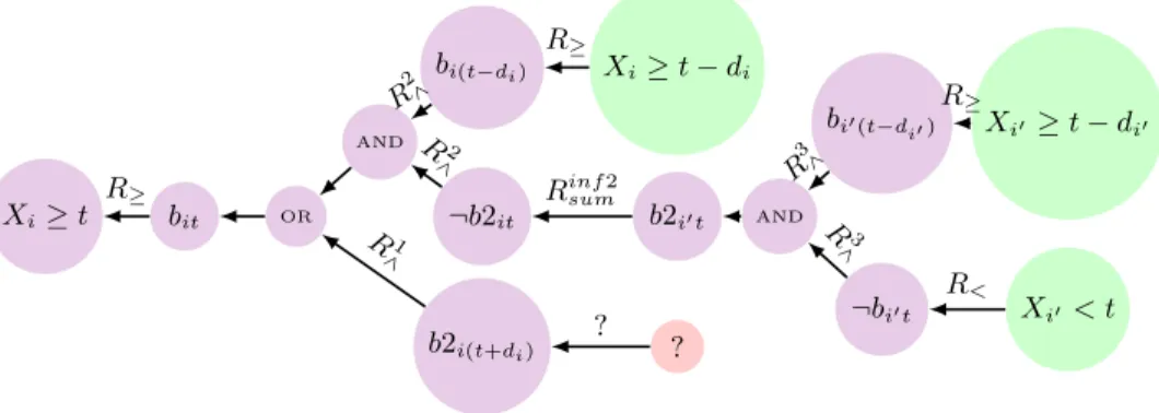
Xi≥ t bit OR AND bi(t−di) Xi≥ t − di ¬b2it b2i0t AND bi0(t−d i0) ¬bi0t Xi0 ≥ t − di0 Xi0< t b2i(t+di) ? R≥ R2∧ R2 ∧ R1 ∧ R≥ Rinf 2 sum ? R3∧ R3 ∧ R≥ R<
Fig. 1. Lower bound event explanation generation
4
6 A. GONTIER et al.
The explanation rule generation is started on a chosen event, for example Xi≥ t. It is found only in the first equation (1), thus the node bit is generated.
The rule that has been used is written on the arrow and the first algorithm is then applied on bit. It appears three times in the decomposition, one in (1) and
two in (2), therefore, there are three possible explanations. The first constraint is forbidden because it was used to get bit. The two other possibilities are labelled
by an OR node. The explanation by the negative variant of bit will generate
an AND node as explained by R2
∧. The generation will continue until we have
no inner decomposition events in the leafs. At the end of this example, there is three leaves in the upper branch and none in the lower one because in this case, there are no rules for a positive variable in a sum less than an constant c with a reified variable set to true (a non reified constraint is implicitly reified to true). We implemented the generator5in the OCaml language. With the decomposi-tion formalism we defined, we can parse the OCaml explanadecomposi-tion rule in LATEX for
them to be read. For example the following generated explanation rules for the Cumulative constraint has been produced by our tool:
Xi≥ t0 t0= t − ci, Xi0≥ t0 t0 = t − ci0, ∀i0, i0 ∈ D, i06= i, i ∈ D, Xi0 < t ∀i0, i0∈ D, i06= i, i ∈ D, Xi≥ t Xi< t0t0= t+ci, Xi0 ≥ t00t00= t0−ci0, t0= t+ci, ∀i0, i0∈ D, i0 6= i, i ∈ D, Xi0 < t0 t0= t + ci, ∀i0, i0∈ D, i06= i, i ∈ D, Xi< t
5
Conclusion
We have presented a generation method for explanations of global constraints, that takes advantage of the constraint decomposition. This method automati-cally expands an implication graph that is run to generate an explanation of an event triggered by the global constraint. The resulting rules can then be encoded within any event-based CDCL-like CP solver. This is still a work in progress, and we plan to explore several questions which are still open. First, we have to extend our implementation to more global constraints, in particular cardinal-ity constraints for which several decompositions exist. We also plan to compare both the expressiveness and the practical efficiency of our generated explanation, compared to the state of the art. The fact that we use a decomposition, which may filter less than the global constraint, may lead to weak explanations, and we will investigate this case. Finally, we already propose a LaTeX generated expres-sion of the explanation in order to help the user refine his/her model. Yet, we have to improve the presentation of this output to obtain a more concise, user-friendly explanations. Since our method is generic, we plan to build a catalog of global constraints explanations as a way to systematically compare different explanations frameworks.
5
https://github.com/ArthurGontierPro/Explanations-by-constraint-decomposition. git
Acknowledgements
The work presented in this article was funded by the French National Re-search Agency as part of the DeCrypt project (ANR- 18-CE39-0007).
References
1. Beldiceanu, N., Carlsson, M., Rampon, J.X.: Global constraint catalog (2010) 2. Bessiere, C., Van Hentenryck, P.: To be or not to be... a global constraint. In:
International conference on principles and practice of constraint programming. pp. 789–794. Springer (2003)
3. Downing, N., Feydy, T., Stuckey, P.J.: Explaining alldifferent. In: Reynolds, M., Thomas, B.H. (eds.) Thirty-Fifth Australasian Computer Science Conference, ACSC 2012, Melbourne, Australia, January 2012. CRPIT, vol. 122, pp. 115– 124. Australian Computer Society (2012), http://crpit.scem.westernsydney.edu. au/abstracts/CRPITV122Downing.html
4. Jussien, N.: The versatility of using explanations within constraint programming. Ph.D. thesis (2003)
5. Khong, M.T., Schaus, C.L.Y.D.P.: R´eification de contraintes tables. JFPC 2016 p. 45 (2016)
6. Montanari, U.: Networks of constraints: Fundamental properties and applications to picture processing. Information sciences 7, 95–132 (1974)
7. Moskewicz, M.W., Madigan, C.F., Zhao, Y., Zhang, L., Malik, S.: Chaff: Engineer-ing an efficient sat solver. In: ProceedEngineer-ings of the 38th annual Design Automation Conference. pp. 530–535 (2001)
8. Narodytska, N.: Reformulation of global constraints. Ph.D. thesis, University of New South Wales, Sydney, Australia (2011), http://handle.unsw.edu.au/1959.4/ 51366
9. Prosser, P.: Hybrid algorithms for the constraint satisfaction problem. Computa-tional intelligence 9(3), 268–299 (1993)
10. Richaud, G.: Outillage logiciel pour les probl`emes dynamiques. Ph.D. thesis (2011),
http://www.theses.fr/2009NANT2145, th`ese de doctorat dirig´ee par Jussien, Narendra Informatique Nantes 2011
11. Rossi, F., Van Beek, P., Walsh, T.: Handbook of constraint programming. Elsevier (2006)
12. Schulte, C., Carlsson, M.: Finite domain constraint programming systems. In: Foundations of Artificial Intelligence, vol. 2, pp. 495–526. Elsevier (2006)
13. Schutt, A., Feydy, T., Stuckey, P.J.: Explaining time-table-edge-finding propaga-tion for the cumulative resource constraint. In: Gomes, C.P., Sellmann, M. (eds.) In-tegration of AI and OR Techniques in Constraint Programming for Combinatorial Optimization Problems, 10th International Conference, CPAIOR 2013, Yorktown Heights, NY, USA, May 18-22, 2013. Proceedings. Lecture Notes in Computer Science, vol. 7874, pp. 234–250. Springer (2013). https://doi.org/10.1007/978-3-642-38171-3 16,https://doi.org/10.1007/978-3-642-38171-3 16
14. Stuckey, P.J.: Lazy clause generation: Combining the power of sat and cp (and mip?) solving. In: International Conference on Integration of Artificial Intelligence (AI) and Operations Research (OR) Techniques in Constraint Programming. pp. 5– 9. Springer (2010)
15. Veksler, M., Strichman, O.: A proof-producing csp solver,a proof supplement. In: Twenty-Fourth AAAI Conference on Artificial Intelligence (2010)