HAL Id: hal-01576857
https://hal.archives-ouvertes.fr/hal-01576857
Submitted on 28 Nov 2017
HAL is a multi-disciplinary open access
archive for the deposit and dissemination of
sci-entific research documents, whether they are
pub-lished or not. The documents may come from
teaching and research institutions in France or
abroad, or from public or private research centers.
L’archive ouverte pluridisciplinaire HAL, est
destinée au dépôt et à la diffusion de documents
scientifiques de niveau recherche, publiés ou non,
émanant des établissements d’enseignement et de
recherche français ou étrangers, des laboratoires
publics ou privés.
Leveraging deep neural networks with nonnegative
representations for improved environmental sound
classification
Victor Bisot, Romain Serizel, Slim Essid, Gael Richard
To cite this version:
Victor Bisot, Romain Serizel, Slim Essid, Gael Richard. Leveraging deep neural networks with
nonneg-ative representations for improved environmental sound classification. IEEE International Workshop
on Machine Learning for Signal Processing MLSP, Sep 2017, Tokyo, Japan. �hal-01576857�
2017 IEEE INTERNATIONAL WORKSHOP ON MACHINE LEARNING FOR SIGNAL PROCESSING, SEPT. 25–28, 2017, TOKYO, JAPAN
LEVERAGING DEEP NEURAL NETWORKS WITH NONNEGATIVE REPRESENTATIONS
FOR IMPROVED ENVIRONMENTAL SOUND CLASSIFICATION
Victor Bisot
‡, Romain Serizel
?§†, Slim Essid
‡, Ga¨el Richard
‡‡
LTCI, T´el´ecom ParisTech, Universit´e Paris - Saclay, F-75013, Paris, France
?Universit´e de Lorraine, LORIA, UMR 7503, Vandœuvre-l`es-Nancy, F-54506, France
§
Inria, Villers-l`es-Nancy, F-54600, France
†
CNRS, LORIA, UMR 7503, Vandœuvre-l`es-Nancy, F-54506, France
ABSTRACT
This paper introduces the use of representations based on non-negative matrix factorization (NMF) to train deep neural net-works with applications to environmental sound classifica-tion. Deep learning systems for sound classification usually rely on the network to learn meaningful representations from spectrograms or hand-crafted features. Instead, we introduce a NMF-based feature learning stage before training deep net-works, whose usefulness is highlighted in this paper, espe-cially for multi-source acoustic environments such as sound scenes. We rely on two established unsupervised and super-vised NMF techniques to learn better input representations for deep neural networks. This will allow us, with simple architectures, to reach competitive performance with more complex systems such as convolutional networks for acoustic scene classification. The proposed systems outperform neu-ral networks trained on time-frequency representations on two acoustic scene classification datasets as well as the best sys-tems from the 2016 DCASE challenge.
Index Terms— Nonnegative Matrix Factorization, Deep Neural Networks, Sound Classification
1. INTRODUCTION
The analysis and classification of sound scenes and events is a rapidly growing area of research. The potential applications, the organization of international challenges [1] and the fre-quent release of new datasets [2] all contribute to its increas-ing success. As for many other sound classification tasks, deep learning is becoming state-of-the-art on an increasing number of sound scene analysis datasets [3, 4]. However, the somewhat limited size of the majority of datasets and the specific challenges of the task contribute to the interest for non-deep learning-based feature learning techniques. Indeed, there are still many datasets where well designed matrix
fac-This work was partly funded by the European Union under the FP7-LASIE project (grant 607480).
torization systems for feature learning can compete with the best neural network systems [5].
In this paper we propose to focus on the acoustic scene classification (ASC) [6]. The main goal of an ASC system is to automatically detect, from recorded soundscapes, the type of location in which the scene takes place, such as a street, in a car or a park. Enabling systems to be aware of their acoustic surroundings has many possible applications such as robotic navigation [7] or surveillance [8]. The first popular way to approach ASC is with feature engineering by building or choosing hand-crafted features adapted to the task. For example, hand-crafted features for ASC are inspired from speech processing with mel frequency cepstral coeffi-cients [9] or from image processing with histogram of ori-ented gradients [10]. The second important trend in ASC is to use feature learning to automatically learn better rep-resentations. Some of the most successful feature learning techniques are based on unsupervised or supervised nonnega-tive matrix factorization (NMF) variants [11, 12, 13]. Finally, ASC is nowadays mainly being addressed with deep neu-ral network-based techniques. Good performance can be ob-tained with simple feed-forward deep neural networks (DNN) [14, 15] but we can also find successful works based on con-volutional neural networks (CNN) [16] and recurrent neural networks (RNN) [17]. While NMF-based feature learning variants using logistic regression as a classifier have recently shown to outperform DNN directly on time-frequency repre-sentations [12], in this paper we propose to take advantage of two well-established approaches to ASC by using NMF-based feature learning techniques to learn better input repre-sentations for DNN. The usual approach to sound classifica-tion with deep learning is to count on the intermediate layers of the network to extract meaningful information for classi-fication from time-frequency representations or even wave-forms [18]. However in ASC, it has been showed that NMF-based feature learning can be competitive with deep learning techniques even when using linear classifiers [13]. Therefore, one can expect that decomposing time-frequency
representa-tions with NMF could better fill the role of the first layer of the network by providing suitable features for the task. In this case, NMF decompositions will be trained separately either using the original unsupervised decompositions [19] or with task-driven NMF (TNMF), a supervised variant of NMF [12]. We evaluate the proposed systems on two of the most used ASC datasets, the DCASE 2016 and 2017 datasets. We will show that training simple DNNs on NMF representations out-performs more complex networks trained on time-frequency representations. Moreover, we obtain state-of-the-art results on the DCASE 2016 challenge set by training networks from TNMF-based representations.
The paper is organized as follows. The motivations and descriptions of our NMF-DNN systems are introduced in Section 2. Experimental results are presented in Section 3. Finally, conclusions and directions for future work are ex-posed in Section 4.
2. NMF DNN SYSTEM
2.1. Representations for ASC
An ASC system is built to predict scene labels from rather long recordings, from 10 seconds up to a few minutes. In this context, training classification models directly from wave-forms can be inefficient [18]. Therefore, the first step of an ASC system is either to compute a time-frequency represen-tation or hand-crafted features in order to work with more compact and interpretable data. Time frequency representa-tions are mostly used as inputs of matrix factorization or CNN systems [12, 13, 16]. They are usually based on perceptually motivated time-frequency representations with log-scaled fre-quency bands such as constant-Q transforms (CQT) or Mel spectrograms.
In the remainder of the paper we refer to fully connected feed-forward neural networks as DNN. When training DNN models for ASC, the dominant approach is still to use hand-crafted features as input of the networks [14, 15]. Such fea-tures, often inspired from other tasks, are built to capture spe-cific aspects of the data. Therefore, they limit by design the information DNN models can learn from such inputs. In that case, the networks mostly play the role of a classifier limit-ing the potential gains from depth or more advanced architec-tures.
2.2. NMF and TNMF
Suppose we have a nonnegative data matrix V ∈ RF ×N+
such as a time-frequency representation of an audio record-ing, where F is the number of frequency bands and N is the number of time frames. The goal of NMF [19] is to find a decomposition that approximates the data matrix V such as: V ≈ WH, with W ∈ RF ×K+ and H ∈ R
K×N
+ . NMF is
obtained solving the following optimization problem:
min D(V|WH) s.t. W, H ≥ 0 (1) where D is a separable divergence and K is the number of components in the decomposition. In this paper D is chosen to be the Euclidean distance. The use of other divergences have not shown to provide any notable increase in perfor-mance for the task [12] while augmenting the computation time.
Supervised NMF models have been applied to ASC with the goal of taking into account the knowledge about the class labels in order to learn better decompositions [12, 13, 20]. We choose to use the Task-driven NMF (TNMF) formula-tion [12], a supervised NMF approach adapted from the Task-driven dictionary learning framework [21]. TNMF learns dis-criminative nonnegative dictionaries by jointly optimizing the NMF and a logistic regression classifier. TNMF can be seen as a DNN with 1 layer acting as a nonnegative projection go-ing into a classification layer with softmax activation.
For both models, once the nonnegative dictionaries are learned from the training data, the data is projected on the dictionaries and the obtained activation matrix contains the features used for classification.
2.3. Motivations
As stated previously, deep learning models have been trained with a wide variety of input representations for ASC, from spectrograms [22] to various cepstral features [15, 23]. De-spite the relative success of nonnegative representations for the task, their potential to improve neural networks perfor-mance has rarely been explored. We believe that NMF-based feature learning is particularity well-suited to train DNN mod-els for ASC.
Firstly, nonnegative decompositions of time-frequency representations can provide flexible and interpretable features to classify sound scenes. Indeed, feature learning techniques have the advantage of adapting to the data and task at hand. Moreover, the interpretability of the decomposition is mainly due to the nonnegative constraints in NMF. Acoustic scenes are multi-source environments containing a wide variety of different acoustic events. It is by identifying the occur-rences of characteristic events that a human can recognize certain environments. Applying NMF decompositions to time-frequency representations for ASC can be interpreted as building a dictionary containing nonnegative frequency representations of basis events. The usefulness of NMF to address certain difficulties of the task has been confirmed as they have been shown to outperform most hand-crafted features. Moreover, it is often easier to train efficient DNNs from time frequency representations than from waveforms. In the same way, we believe that learning networks from NMF-based features could be even simpler.
Secondly, the unsupervised NMF feature learning stage acts as a first pre-trained layer of the network. Here, NMF plays a similar role to established layer-wise pre-training techniques [24, 25], with the goal of augmenting the general-ization power of the network by training its weights according to a data reconstruction loss (mean squared error). Just as a regular fully-connected layer, NMF has a matrix of weights W (the dictionary) and the nonnegative projection on those weights corresponds to the output of the layer’s activations (after a ReLU or softplus activation function). The most common activation function in DNN is the ReLU activation which provides sparse nonnegative representations. Capital-izing on this and contrary to conventional usage of neural networks, the weights here are constrained to be nonnegative and the activation function is the solution of a nonnegative sparse coding problem. In our case, we fix the first layer as nonnegative projections on a dictionary learned by solving the unsupervised problem equation (1). Other works in this direction also proposed to build simple auto-encoders that mimic the behavior of NMF decompositions [26] or to unfold the multiplicative update algorithm of NMF in order to build a deep NMF model [27].
2.4. Classifiers
Mostly due to the nature of the task and the size of the datasets, more complex neural networks such as CNN and RNN have not yet become dominant in ASC, unlike in other sound classification tasks. Indeed, good performance can be obtained with simple DNNs trained on appropriate represen-tations [14]. Moreover, NMF-based systems using logistic regression (LR) as a classifier has proven to provide com-petitive performances with deeper architectures trained on time frequency representations. In this work, we use standard architectures for the system to keep the focus on the input representations. Both the NMF and time-frequency repre-sentations will be considered as input to simple classifiers, e.g. with simple multi-layer perceptrons with fully connected layers (DNN).
3. EXPERIMENTAL EVALUATION
3.1. Datasets
We use the 2016 and 2017 versions of the DCASE challenge datasets for acoustic scene classification [1]. They respec-tively contain 10 and 13 hours of urban audio scenes recorded with binaural microphones in 15 different environments. We use the same 4 training-test splits provided by the challenge, where 25% of the examples are kept for testing. The 2016 and 2017 datasets have all labels and some recordings in common, the main difference is the length of the recordings to classify: 30-s long recordings for the DCASE 2016 and 10-s record-ings for the 2017 version. Finally, we also exploit the sep-arate challenge subset for the DCASE 2016 dataset, used to
Dcase 2016 Dcase2017 Layers Units Layers Units
CQT 3 256 3 512
NMF 2 256 2 256
Table 1. Best number of hidden layers and units per layer with CQT and NMF representations for both datasets.
rank the submitted systems, which contains 390 scene record-ings of 30 seconds. In that case, our systems are trained on the full DCASE 2016 dataset and tested on the challenge subset.
3.2. Experimental setup
Time-frequency representations: We take advantage of previous works on NMF for ASC to choose an appropriate time-frequency representation [28]. We extract Constant-Q transforms with 24 bands per octave from 5 to 22050 Hz and with 30-ms non-overlapping windows using YAAFE [29]. The time frequency representations are then averaged by slices of 1 second resulting in 30 or 10 vectors per example for the 2016 and 2017 dataset respectively. After concatenat-ing all the averaged slices for each example to build the data matrix, we apply a square root compression to the data and scale each feature dimension to unit variance.
NMF setting: For the unsupervised NMF systems, we learn nonnegative dictionaries for each fold by solving the optimization problem in equation (1) on the training set. We perform NMF on 10 different random initializations and keep the dictionary that provided the lowest reconstruction cost. The same dictionaries will be used as initializations of TNMF and to obtain the projections used as input of the DNN-NMF systems. We use the GPU implementation of multiplicative update rules presented by [30].
TNMF setting: For TNMF, we keep the same parameters as for one of the challenge submissions [28]. The gradient step is set to 0.001, the classifier regularization to 0.1 and the sparsity to 0.2. We stop the learning after 6 iterations and keep the dictionaries to initialize some of the networks. The TNMF model is trained with logistic regression (TNMF-LR). Once the model is trained, the dictionaries are fixed and used to compute the input representation for the TNMF-DNN system.
DNN setting: We use simple feed-forward fully-connected layers with Rectified linear unit activations (ReLU) [31]. Dropout with probability of 0.2 is applied to each hidden layer [32]. The output layer has a softmax activation and the cost function is the categorical cross-entropy. Such architec-tures have proven to be sufficient to build good ASC systems [15, 14]. In the training stage, each averaged slice, is consid-ered as a separate data point. During testing we perform late fusion by averaging the outputs of the network for each slice coming from the same example in order to take a decision on
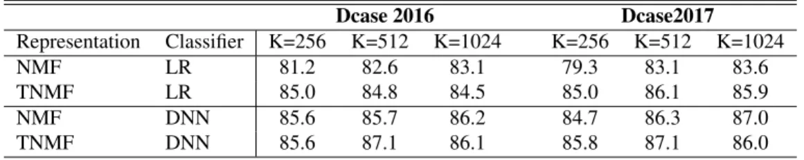
Dcase 2016 Dcase2017 Representation Classifier K=256 K=512 K=1024 K=256 K=512 K=1024 NMF LR 81.2 82.6 83.1 79.3 83.1 83.6 TNMF LR 85.0 84.8 84.5 85.0 86.1 85.9 NMF DNN 85.6 85.7 86.2 84.7 86.3 87.0 TNMF DNN 85.6 87.1 86.1 85.8 87.1 86.0
Table 2. Accuracy results for NMF and TNMF systems on the two ASC datasets for different dictionary sizes K
Dcase 2016 Dcase2017 Baseline system [1] 72.5 74.8 CQT-LR 77.3 78.3 NMF-LR 83.1 83.6 CQT-DNN 82.8 84.5 NMF-DNN 86.2 87.0 TNMF-DNN 87.1 87.1
Table 3. Best results for each representation with logistic re-gression classifier and DNN compared to the baseline sys-tems.
the full recording.
DNN parameter search: We perform a parameter search to find the best number of layers and units for both possible input presentations and datasets. To do so, we create a de-velopment set from each of the 4 training sets and keep the parameters that give the best average results over all develop-ment sets. The number of hidden layers is chosen in {0, 1, 2, 3} and the number of hidden units in {128, 256, 512, 1024}. Once the best parameters are found, the system is trained on the full training set, including the previously extracted devel-opment set. The best values for each setting can be found in Table 1. The networks are trained with Keras [33] on Tesla K80 GPUs using stochastic gradient descent on 100 epochs with the default settings. Changing the training algorithm or its parameters have not provided any notable increase in per-formance.
3.3. Results
3.3.1. Classifying NMF representations
We start by presenting the accuracy percentage results for the NMF-based systems in Table 2. First, the performance of unsupervised NMF-based systems confirmed the useful-ness of DNN to classify such nonnegative representations. In fact, on both datasets, neural networks can provide more than 3% accuracy improvements compared to logistic regression. Then, the NMF-DNN allows us to get slightly improved per-formance compared to the TNMF-LR, which suggests inter-preting unsupervised features with DNN can be a viable alter-native to more complex supervised matrix factorization tech-niques. Finally, we can benefit from the supervised
dictionar-ies learned with TNMF to further improve the performance of the neural networks. As for logistic regression, using more discriminative representations from TNMF lowers the num-ber of components required to get performance that is similar to the unsupervised systems.
3.3.2. Comparing to time-frequency representations
We compare in Table 3 the best proposed NMF-DNN systems to similar networks using the CQT representation directly as input. We also include the results for each dataset baseline systems [1]. They both are based on Mel energy represen-tations classified with Gaussian mixture models for the 2016 dataset and DNN for the 2017 dataset. We also propose to di-rectly classify the CQT representation with logistic regression in order to show the quality of this time-frequency representa-tion for the task as it largely outperforms the baseline systems. The first interesting result to note is the similar performance of NMLF-LR and CQT-DNN systems. Indeed, this shows that NMF can fill the role of the first layer of the network to learn suitable representations. Both starting from the CQT, unsupervised NMF feature learning with logistic regression and CQT-DNN have less than 1% accuracy differences. The second important result is the comparison of CQT and NMF representations as inputs of DNN. In fact, learning deep neu-ral networks from NMF features reaches up to 3.6% accuracy improvement over the CQT input. Finally it is also interest-ing to note that, on both datasets, DNN with NMF as input requires one less hidden layer as well as less units for the DCASE 2017 dataset, as presented in Table 1. This goes in the direction of interpreting NMF as a first layer of the net-work discussed in Section 2.2 by being better at performing similar tasks. It confirms the intuition that NMF can better fill the role of intermediate representation learning of the first layer in a standard DNN.
3.3.3. Results on the Dcase 2016 challenge set
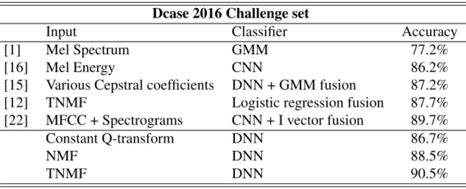
Finally we compare in Table 4 the proposed systems to several of the best performing submissions to the DCASE 2016 chal-lenge dataset, including the best ranked system [22]. We have kept the same network architectures and parameters as for the DCASE 2016 development dataset to compute the results on the challenge set. The proposed CQT-DNN already reaches recognition results similar to the best CNN system introduced
Dcase 2016 Challenge set
Input Classifier Accuracy
[1] Mel Spectrum GMM 77.2%
[16] Mel Energy CNN 86.2%
[15] Various Cepstral coefficients DNN + GMM fusion 87.2% [12] TNMF Logistic regression fusion 87.7% [22] MFCC + Spectrograms CNN + I vector fusion 89.7% Constant Q-transform DNN 86.7%
NMF DNN 88.5%
TNMF DNN 90.5%
Table 4. Accuracy scores on the separate DCASE 2016 challenge test set compared to the best state-of-the-art methods.
by [16]. It further confirms that simple DNN architectures can be sufficient to deal with ASC. Moreover, as previously, using the NMF-DNN and TNMF-DNN systems is confirmed to out-perform the CQT-DNN systems. The advantages of training the representations with TNMF is even clearer in this setting as it allows for a 2%-accuracy improvement. Moreover it also slightly improves performance compared the best ranked sub-mission on this dataset [22]. It is also important to note that most of the best ranked systems rely on some form of fusion between different classifiers. Instead we have proposed a sim-pler but competitive system by making choices adapted to the task at hand. Further improvement can than be expected by considering fusion paradigms.
4. CONCLUSION
In this work, we have proposed simple neural network-based systems to classify nonnegative representations for acoustic scene classification. We have discussed the benefits of us-ing NMF-based features as input of DNN models instead of time-frequency representations or hand-crafted features. An experimental evaluation on two standard ASC datasets high-lighted the usefulness of NMF to build more efficient and bet-ter performing ASC systems. Relying on supervised NMF representations from TNMF allowed us to outperform pre-vious state-of-the-art methods, including DNN and CNN fu-sion based methods, resulting in the best performance on the DCASE 2016 challenge dataset. Interesting perspectives for future work could include studying in what respect the size of datasets has an influence on the performance of NMF-based systems as well as if the NMF representation can be jointly learned with the networks.
5. REFERENCES
[1] A. Mesaros, T. Heittola, and T. Virtanen, “Tut database for acoustic scene classification and sound event detection,” in Proc. of European Signal Processing Conference, 2016. [2] J. F. Gemmeke, D. P. W. Ellis, D. Freedman, A. Jansen,
W. Lawrencee, R. C. Moore, M. Plakal, and M. Ritter, “Audio set: An ontology and human-labeled dataset for audio events,” in Proc. of International Conference on Acoustics, Speech and Signal Processing, 2017.
[3] J. Salamon and J. P. Bello, “Deep convolutional neural net-works and data augmentation for environmental sound classi-fication,” IEEE Signal Processing Letters, vol. 24, no. 3, pp. 279–283, 2017.
[4] G. Parascandolo, H. Huttunen, and T. Virtanen, “Recurrent neural networks for polyphonic sound event detection in real life recordings,” in Proc. of International Conference on Acoustics, Speech and Signal Processing, 2016.
[5] T. Komatsu, T. Toizumi, R. Kondo, and Y. Senda, “Acous-tic event detection method using semi-supervised non-negative matrix factorization with a mixture of local dictionaries,” Tech. Rep., DCASE2016 Challenge, 2016.
[6] D. Barchiesi, D. Giannoulis, D. Stowel, and M. D. Plumbley, “Acoustic scene classification: Classifying environments from the sounds they produce,” IEEE Signal Processing Magazine, vol. 32, no. 3, pp. 16–34, 2015.
[7] S. Chu, S. Narayanan, C.-C. J. Kuo, and M. J. Mataric, “Where am i? scene recognition for mobile robots using audio fea-tures,” in Proc. of International Conference on Multimedia and Expo, 2006, pp. 885–888.
[8] R. Serizel, V. Bisot, S. Essid, and G. Richard, “Machine lis-tening techniques as a complement to video image analysis in forensics,” in Proc. International Conference on Image Pro-cessing, 2016, pp. 5470–5474.
[9] A. J. Eronen, V. T. Peltonen, J. T. Tuomi, A. P. Klapuri, S. Fagerlund, T. Sorsa, G. Lorho, and J. Huopaniemi, “Audio-based context recognition,” IEEE Transactions on Audio, Speech, and Language Processing, vol. 14, no. 1, pp. 321–329, 2006.
[10] A. Rakotomamonjy and G. Gasso, “Histogram of gradients of time-frequency representations for audio scene classification,”
IEEE/ACM Transactions on Audio, Speech and Language Pro-cessing (TASLP), vol. 23, no. 1, pp. 142–153, 2015.
[11] E. Benetos, M. Lagrange, and S. Dixon, “Characterisation of acoustic scenes using a temporally constrained shift-invariant model,” in Proc. of Digital Audio Effects, 2012.
[12] V. Bisot, R. Serizel, S. Essid, and G. Richard, “Feature learn-ing with matrix factorization applied to acoustic scene classifi-cation,” IEEE/ACM Transactions on Audio, Speech, and Lan-guage Processing, vol. 25, no. 6, pp. 1216–1229, June 2017. [13] A. Rakotomamonjy, “Supervised representation learning for
audio scene classification,” IEEE/ACM Transactions on Audio, Speech, and Language Processing, vol. 25, no. 6, pp. 1253– 1265, 2017.
[14] J. Li, W. Dai, F. Metze, S. Qu, and S. Das, “A comparison of deep learning methods for environmental sound,” arXiv preprint arXiv:1703.06902, 2017.
[15] S. Park, S. Mun, Y. Lee, and H. Ko, “Score fusion of classi-fication systems for acoustic scene classiclassi-fication,” Tech. Rep., DCASE2016 Challenge, September 2016.
[16] M. Valenti, A. Diment, G. Parascandolo, S. Squartini, and T. Virtanen, “DCASE 2016 acoustic scene classification us-ing convolutional neural networks,” Tech. Rep., DCASE2016 Challenge, 2016.
[17] H. Phan, P. Koch, F. Katzberg, M. Maass, R. Mazur, and A. Mertins, “Audio scene classification with deep recurrent neural networks,” arXiv preprint arXiv:1703.04770, 2017. [18] W. Dai, C. Dai, S. Qu, J. Li, and S. Das, “Very deep
convo-lutional neural networks for raw waveforms,” arXiv preprint arXiv:1610.00087, 2016.
[19] D. D. Lee and H. S. Seung, “Learning the parts of objects by non-negative matrix factorization,” Nature, vol. 401, no. 6755, pp. 788–791, 1999.
[20] A. Mesaros, T. Heittola, O. Dikmen, and T. Virtanen, “Sound event detection in real life recordings using coupled matrix fac-torization of spectral representations and class activity annota-tions,” in Proc. IEEE International Conference on Acoustics, Speech and Signal Processing, 2015, pp. 151–155.
[21] J. Mairal, F. Bach, and J. Ponce, “Task-driven dictionary learn-ing,” IEEE Transactions on Pattern Analysis and Machine In-telligence, vol. 34, no. 4, pp. 791–804, 2012.
[22] H. Eghbal-Zadeh, B. Lehner, M. Dorfer, and G. Widmer, “CP-JKU submissions for DCASE-2016: a hybrid approach using binaural i-vectors and deep convolutional neural networks,” Tech. Rep., DCASE2016 Challenge, September 2016. [23] Y. Petetin, C. Laroche, and A. Mayoue, “Deep neural
net-works for audio scene recognition,” in Proc. European Signal Processing Conference, 2015, pp. 125–129.
[24] Y. Bengio, P. Lamblinl, D. Popovici, H. Larochelle, et al., “Greedy layer-wise training of deep networks,” Advances in neural information processing systems, vol. 19, pp. 153, 2007. [25] G. E. Hinton, S. Osindero, and Y.-W. Teh, “A fast learning algorithm for deep belief nets,” Neural computation, vol. 18, no. 7, pp. 1527–1554, 2006.
[26] P. Smaragdis and S. Venkataramani, “A neural network alternative to non-negative audio models,” arXiv preprint arXiv:1609.03296, 2016.
[27] J. Le Roux, J.R. Hershey, and F. Weninger, “Deep nmf for speech separation,” in Proc. of International Conference on Acoustics, Speech and Signal Processing. IEEE, 2015, pp. 66– 70.
[28] V. Bisot, R. Serizel, S. Essid, and G. Richard, “Supervised non-negative matrix factorization for acoustic scene classification,” Tech. Rep., DCASE2016 Challenge, September 2016. [29] B. Mathieu, S. Essid, T. Fillon, J. Prado, and G. Richard,
“Yaafe, an easy to use and efficient audio feature extraction software.,” in Proc. of International Society for Music Infor-mation Retrieval, 2010, pp. 441–446.
[30] R. Serizel, S. Essid, and G. Richard, “Mini-batch stochastic approaches for accelerated multiplicative updates in nonneg-ative matrix factorisation with beta-divergence,” in Machine Learning for Signal Processing (MLSP), 2016 IEEE 26th In-ternational Workshop on. IEEE, 2016, pp. 1–6.
[31] K. Jarrett, K. Kavukcuoglu, M. Ranzato, and Y. LeCun, “What is the best multi-stage architecture for object recognition?,” in Proc. IEEE International Conference on Computer Vision, 2009, pp. 2146–2153.
[32] G. E. Hinton, N. Srivastava, A. Krizhevsky, I. Sutskever, and R. R. Salakhutdinov, “Improving neural networks by pre-venting co-adaptation of feature detectors,” arXiv preprint arXiv:1207.0580, 2012.