HAL Id: hal-00442765
https://hal.archives-ouvertes.fr/hal-00442765
Submitted on 22 Dec 2009
HAL is a multi-disciplinary open access
archive for the deposit and dissemination of
sci-entific research documents, whether they are
pub-lished or not. The documents may come from
teaching and research institutions in France or
abroad, or from public or private research centers.
L’archive ouverte pluridisciplinaire HAL, est
destinée au dépôt et à la diffusion de documents
scientifiques de niveau recherche, publiés ou non,
émanant des établissements d’enseignement et de
recherche français ou étrangers, des laboratoires
publics ou privés.
nonlinear mixtures of finite-alphabet sources
Marc Castella
To cite this version:
Marc Castella. Inversion of polynomial systems and separation of nonlinear mixtures of finite-alphabet
sources. IEEE Transactions on Signal Processing, Institute of Electrical and Electronics Engineers,
2008, 56 (8 (Part 2)), pp.3905 - 3917. �10.1109/TSP.2008.921788�. �hal-00442765�
Inversion of polynomial systems and separation of
nonlinear mixtures of finite-alphabet sources
Marc Castella
IT/TELECOM SudParis/D´epartement CITI/UMR-CNRS 5157
9 rue Charles Fourier, 91011 Evry Cedex - France
e-mail: marc.castella@it-sudparis.eu
Tel: +33 1 60 76 41 71
Fax: +33 1 60 76 44 33
Abstract— In this contribution, Multi-Input Multi-Output (MIMO) mixing systems are considered, which are instantaneous and nonlinear but polynomial. We first address the problem of invertibility, searching the inverse in the class of polynomial systems. It is shown that Groebner bases techniques offer an attractive solution for testing the existence of an exact inverse and computing it.
By noticing that any nonlinear mapping can be interpolated by a polynomial on a finite set, we tackle the general nonlinear case. Relying on a finite alphabet assumption of the input source signals, theoretical results on polynomials allow us to represent nonlinear systems as linear combinations of a finite set of monomials. We then generalize the first results to give a condition for the existence of an exact nonlinear inverse. The proposed method allows to compute this inverse in polynomial form.
In the light of the previous results, we go further to the blind source separation problem. It is shown that for sources in a finite alphabet, the nonlinear problem is tightly connected with both problems of underdetermination and of dependent sources. We concentrate on the case of two binary sources, for which an easy solution can be found. By simulation, this solution is compared to techniques borrowed from classification methods.
Index Terms— nonlinear systems, polynomials, Groebner bases, blind source separation, finite alphabet
I. INTRODUCTION
For the last decades, deconvolution and signal restoration issues have been active research fields. In a multidimensional context for instance, the problem of source separation has received considerable attention [9], [11], [33], [30], [7]. It consists in the restoration of several original signals from the observation of several mixtures of them. Depending on context, different approaches may be considered: if a strong information on the mixing system is available, then non-blind separation methods can be developped based on this information. On the contrary, blind methods do not assume any a priori knowledge of the mixing system but they generally rely on the strong assumption of statistical independence of the source signals: this is the case in “Independent Component Analysis” (ICA) which is now a well recognized concept which corresponds to blind separation of an instantaneous linear mixture. Recently, other models have been considered, such as convolutive [12], [42], [39] or nonlinear ones [45], [31], [24].
In this paper, the case of a nonlinear mixture is tackled. More precisely, the aim is to answer the following two
questions: (i) Does an inverse exist for a given nonlinear mixture? (ii) If yes, propose a method for blind recovery of the nonlinearly mixed sources. Both questions are obviously challenging and are tackled in a restricted context that allows to give an answer: polynomial nonlinearities are assumed to answer (i) and a finite-alphabet assumption is added to deal with (ii).
In the linear context, perfect invertibility conditions of Multi-Input/Multi-Output (MIMO) linear time invariant sys-tems are well-known and they reduce to left-invertibility of matrices. The elements of the mixing and separating matrix are either scalars in the instantaneous case, or polynomials in the case of MIMO finite impulse response (FIR) filters. Polynomials in the matrices may have several variables in the case where multi-dimensional (e.g. images) and multi-channel signals are considered (see e.g. [43], [49]). On the other hand, we are not aware of any such general result in the nonlinear case, although previous results include [3], which presents an invertibility criterion but no method for computing the inverse and [10] for a particular class of nonlinear systems. The gen-eral class of nonlinear systems is often too wide to enable us to deal with the associated problem and we should preferably try to restrict to a smaller class of systems. Obtaining perfect invertibility conditions on a class of nonlinear mixtures will help considering such models in a blind context [29], [20]. This motivates our interest for polynomial systems, which to a certain extent can be considered as one of the simplest form of nonlinearity. In the first part of this paper we show that methods exist which allow to compute a polynomial inverse (if it exists) of a polynomial MIMO mixing system. We illustrate their validity and effectiveness through examples.
The blind source separation problem serves as an example of the utility of the previous considerations. This issue still faces unanswered questions, in particular in the nonlinear case, although this case has already been addressed [45], [2]. Generally, specific structures have been assumed on the nonlinear mixture: indeed, a general nonlinear mixture of independent sources cannot be identified without additionnal constraint on the mixture. For example, a conformal mapping is assumed in [31]. First published in [35], more general results concerning identifiability of a large class of nonlinearities satisfying an addition theorem have been pointed out recently in [21], [34]. Other structures have been introduced; the post-nonlinear one is probably one of the most popular [45], [32],
[36], [22], [5], [4], [6]. On the other hand, the case of sources in a discrete or finite alphabet has been considered for long [37], [47], [23], [25] and the strength of the discrete sources assumption has been recognized. It indeed allows to relax some usual assumptions, such as the statistical independence of the sources [38], or to deal with underdetermined mixtures —that is mixtures with more sources than sensors— [40], [13], [17], [19]. However the nonlinear source separation problem seems still open for discrete sources, although a geometrical approach may appear as well suited [1]. In this paper, we show how results from commutative algebra give more insight in the case of nonlinear mixtures. We then propose a solution to blind separation in the simple case of binary sources.
The new and original points in the paper are the following:
• We use tools borrowed from commutative algebra. These
powerful tools seem still ignored in the signal processing community although they have been successfully applied in many contexts (e.g. statistics [44], channel identifi-cation [25]). We translate and apply the corresponding results in a MIMO source separation context.
• We propose an equivalent linear model for any nonlinear
MIMO mixture of finite-alphabet sources.
• We apply the previous methods to the case of blind
separation of binary sources: in our particular case, a separation is surprisingly obtained although the sources of the equivalent linear model are not independent. Section II describes the issue which is addressed in the paper. Necessary mathematical tools and definitions are introduced in Section III. Section IV explains how to compute a polynomial inverse. If it does not exist, an alternative solution is shortly discussed. Section V is concerned with the case of finite alphabet sources. It is shown how an equivalent linear model can be used by introducing virtual sources. The invertibility issue is also addressed. Section VI is concerned with the nonlinear blind source separation problem of two binary sources. It is shown that in specific situations, ICA techniques can be successful although the virtual sources introduced by the equivalent linear model are dependent. Finally, Section VII concludes the paper. All examples which have been computed can be reproduced using Appendix III.
Throughout the paper, K denotes a field (the complex numbers C or the real numbers R or possibly any subfield of C). K[s] is the set of polynomials with coefficients in K and variables s = (s1, . . . , sN). E{.} is the mathematical
expectation of any random variable and Cum {.} stands for the cumulant of a set of random variables.
II. PROBLEM STATEMENT
A. Source separation
We consider a set of Q sensors acquiring Q observation signals which compose the vector valued signal (x(n))n∈Z=
((x1(n))n∈Z, . . . , (xQ(n))n∈Z)
T
. In a source separation con-text, one assumes that these observations come from an-other set of signals, called the sources and denoted by the vector (s(n))n∈Z , ((s1(n))n∈Z, . . . , (sN(n))n∈Z)
T
. Both the observations and the sources may be real or complex-valued signals. We assume a deterministic relation between
the sources and the observations. More precisely, the paper focuses on instantaneous nonlinear transforms of the sources. Dropping the time index n, we thus write x = f (s) where f is a nonlinear function, f : KN → KQ. Componentwise, the
corresponding mixing equations read: x1 = f1(s1, . . . , sN) .. . ... xQ = fQ(s1, . . . , sN) (1) where f1, . . . , fQ constitute the components of f .
The source separation problem consists in recovering the sources s1, . . . , sN from the observations x1, . . . , xQ. This is
equivalent to finding the inverse MIMO system g : KQ →
KN. In other words, we look for the components g
i : KQ→ K
of g = f−1 such that for all i:
si= gi(x1, . . . , xQ). (2)
The first contribution of this paper addresses the problem of computing an inverse for a known and given mixing system such as (1).
In the case where no information is available on the mixing system (1), the separation problem is referred to as the
blind source separation problem. This issue, which consists in
estimating the sources from the observations only, is addressed in the case of binary sources.
B. Nonlinear functions and polynomials
This paper focuses on the particular case where the func-tions fi, i ∈ {1, . . . , Q} in (1) are polynomials, that is for all i,
fi∈ K[s]. This restriction is partly justified by the difficulty to
tackle the nonlinear case because of its generality. In addition, polynomials constitute an important class of nonlinear models which may represent acceptable approximations of certain nonlinearities. Finally, an important reason to deal with this model is the following one.
Consider the case where the multidimensional source vector belongs to a finite set: s ∈ A = {a(1), . . . , a(na)}. Although
seemingly restrictive, this situation is highly interesting since it occurs in digital communications, where the emitted source sequences belong to a finite alphabet depending on the mod-ulation used.
An important observation is that if s ∈ A and A is finite,
all instantaneous mixtures of the sources can be expressed as polynomial mixtures. This follows immediately from the fact
that any function on a finite set can be interpolated by a poly-nomial in a way similar to Lagrange polypoly-nomial interpolation [16]. It follows that polynomial mixtures constitute the general model of nonlinear mixtures in the case of sources belonging to a finite alphabet. On the other hand, one should notice that the well-known post-nonlinear model is not easier to deal with in the case of finite alphabet sources [36]: generically, a scalar variable which is a linear combination of discrete sources has a number of distinct values equal to the number of possible states of the source vector. Each of these distinct values can be freely mapped to any value: hence one can see that in the generic case, and for finite alphabet sources, any nonlinear mapping can be represented by a post-nonlinear mapping, which makes both problems equivalent.
III. MATHEMATICAL PRELIMINARIES
A. Definitions
Assuming that the model (1) is polynomial, and in order be able to resort to algebraic techniques, we will restrict the sep-arator to the class of polynomial functions in x1, . . . , xQ, that
is: ∀i, gi∈ K[x]. Then, algebra and Groebner basis techniques
are powerful methods for the study of multivariate polynomi-als. They have been applied only recently in signal processing [41], [49], [46]. It is out of the scope of this paper to explain the associated notions (see [15] for a detailed introduction to the subject) but we recall some basic definitions required here for comprehension. We will introduce the definitions in K[s]. In the following, boldface letters denote N -tuples and for any
α ∈ NN we write: sα, sα1
1 . . . sαNN.
Definition 1: Let h1, . . . , hp ∈ K[s] be polynomials. The
ideal generated by these polynomials in K[s] is the subset of K[s] which consists of all linear combinations a1h1+ . . . +
aphp where a1, . . . , ap are polynomials in K[s]. It is denoted
by hh1, . . . , hpi.
Definition 2: A monomial ordering ≺ on K[s] is a total
ordering relation on the set of monomials such that:
• if sα≺ sβ then sα+γ ≺ sβ+γ
• ≺ is a well-ordering, that is, every nonempty collection
of different monomials has a smallest element under ≺. A simple example of monomial ordering is the lexicographic order, where by definition sα≺ sβ if and only if in the vector
difference β − α, the left-most nonzero entry is positive. Here is a set of monomials illustrating this order in K[s1, s2]:
1 ≺ s2≺ s22≺ . . .
≺ s1≺ s1s2≺ s1s22≺ . . . ≺ s21≺ s21s2≺ . . .
Given a monomial ordering, for a polynomial which reads
h = Pαcαxα, its leading term is defined by LT(h) =
cαxα where cα is referred to as the leading coefficient and
xα, called the leading monomial, is the largest monomial
appearing in h in the ordering ≺. Then, we can also define a division algorithm, which generalizes the division algorithm in the case of one variable:
Theorem 1 (division algorithm): Let (h1, . . . , hp) be an
or-dered p-tuple of polynomials. Every polynomial h can be written as:
h = a1h1+ . . . + aphp+ r (3)
where ai, hi are polynomials and r is a linear combination
with coefficients in K of monomials, none of which is divisible by any leading term of h1, . . . , hp. (possibly, r = 0).
If we consider the ideal I = hh1, . . . , hpi, the division
algorithm provides a way to write any polynomial as the sum
h = hI+ r where hI lies in I and no term of r is divisible
by any of the leading terms of h1, . . . , hp. Unfortunately, the
remainder r in this decomposition is not unique in general. A remarkable exception is when the set of generators satisfy the following definition.
Definition 3: The set {h1, . . . , hp} is a Groebner basis of
the ideal I = hh1, . . . , hpi if and only if the remainder r in
(3) is uniquely determined for all h ∈ K[s].
Importantly, there exist an algorithm, initially developped by Buchberger for converting a given generating set to a Groebner basis [8]. For a given ideal I, there may exist several Groebner bases, which justifies that the notion of reduced Groebner basis is introduced.
Definition 4: A reduced Groebner basis for a polynomial
ideal I is a Groebner basis G for I such that for all h in G:
• the leading coefficient of h is 1.
• no monomial of h lies in the ideal hLT(G − {h})i
gen-erated by the leading terms of the set G − {h}.
For a given monomial ordering, any ideal different from {0} has a unique reduced Groebner basis.
B. Example
We illustrate the previous definitions: consider h1= s1s2−
s1+ 1, h2= s22− 1 and h = s1s2− s1+ s2+ 2 in K[s1, s2]
with lexicographic order. We define the ideal I = hh1, h2i. A
possible remainder after division of h by (h1, h2) is s2+ 1
since indeed h = 1.h1+ 0.h2+ (s2+ 1) and neither s2nor 1
can be divided by LT(h1) or LT(h2).
However, non uniqueness of the remainder can be observed writing h = (s2+ 2).h1− s1.h2. This is no surprise because
the set {h1, h2} is not a Groebner basis for I, which is related
to the fact that s2+ 1 = (s2+ 1).h1− s1.h2is a polynomial
with leading term lower than the leading terms of h1 and h2
(note indeed that a cancelling of the leading terms occured). Going further, one can write −2s1+ 1 = h1− s1.(s2+ 1) =
(−s1s2−s1+1).h1+s21.h2. Hence −2s1+1 and s2+1 belong
to I and one can prove {−2s1+ 1, s2+ 1} is a Groebner basis
of I. So is any set of polynomials in I set containing these two polynomials. The reduced Groebner basis of I is the set
{s1− 1/2, s2+ 1}.
IV. INVERTIBILITY
Based on the previous notions, we show that existing results can be used to find a polynomial inverse to a given poly-nomial MIMO system. Another question of great importance would be to find a generic condition or a minimum number of equations to ensure invertibility or separability as defined in Section IV-B. This question will not be treated here and still remains open. Finally, the reader should notice that the results presented in this section require the exact knowledge or a prior identification of the mixing system.
A. Perfect invertibility
The problem of finding a polynomial gi such that (2) is
satisfied is a particular case of the subalgebra or subring mem-bership problem [15], [26]: to see this, we shall now put our problem differently and precise some notations.
In the present context of non blind inversion, the polyno-mials fi ∈ K[s], i ∈ {1, . . . , Q} are given, and the inversion
condition (2) should be written correctly
si= gi(f1(s), . . . , fQ(s)). (4)
For ease of notation, we will no longer write explicitly the dependence of f1, . . . , fQ in s. Restricting ourself to
f1, . . . , fQ with coefficients in K. Let K[f ] be the subset of
K[s] consisting of all such expressions. Introduce the variables
x1, . . . , xQ (of course, they will represent the observations)
and consider the set K[x] of polynomials in these variables. Any element of K[f ] can be obtained by sustituting f1, . . . , fQ
for x1, . . . , xQin a polynomial of K[x]. Then, the initial
prob-lem amounts to saying whether si ∈ K[f ] or equivalently
whether a polynomial gi∈ K[x] exists or not such that (4) is
satisfied. The answer is provided by the following theorem [15, p.334] which requires to work in the set K[s, x] of polynomials in the variables s1, . . . , sN, x1, . . . , xQ:
Theorem 2: Fix a monomial ordering in K[s, x] where any
monomial involving one of s1, . . . , sN is greater than all
mono-mials in K[x]. Let G be a Groebner basis of the ideal hf1−
x1, . . . , fQ − xQi ⊂ K[x, s]. Given h ∈ K[s], let g be the
remainder of h on division by G. Then: 1) h ∈ K[f ] if and only if g ∈ K[x].
2) if h ∈ K[f ], then h = g(f1, . . . , fQ) is an expression of
h as a polynomial in f1, . . . , fQ.
Monomial orderings satisfying the condition in the above the-orem are called elimination orderings for s1, . . . , sN. One
should note that this condition is satisfied by the lexicographic order in K[s, x] but other monomial orderings also satisfy this condition [15]. The invertibility result will not depend on the chosen ordering, but different inverses may be found. The method for perfect inversion with a polynomial separator then follows from the above proposition which can be applied successively to the polynomials s1, . . . , sN in K[s]. It reads:
1) Choose in K[s, x] an elimination ordering for s1, . . . , sN
and define I = hf1− x1, . . . , fQ− xQi.
2) Compute a Groebner basis G of I.
3) For i = 1 . . . N , compute the division of si by G. If
the remainder gi of the division is in K[x], we have
si = gi(f1, . . . , fQ) (that is, gi satisfies (2)),
other-wise, si cannot be recovered exactly by a polynomial
in f1, . . . , fQ.
1) Example: Throughout the paper, we will consider the
example provided by the following equations: x1= f1(s1, s2) = 3s21+ 2s1s2+ 4s22+ 7s1+ 4s2 x2= f2(s1, s2) = −3s21+ 5s1s2+ 2s1+ s2 x3= f3(s1, s2) = −3s1+ 6s2 x4= f4(s1, s2) = 6s21− s1s2+ 4s22+ 3s1− 9s2 (5)
Groebner basis computation and polynomial division are im-plemented in many computer algebra systems. Using the lex-icographic order in K[s1, s2, x1, x2, x3, x4], the following
in-verse of (5) has been computed (see Appendix III): (
s1=14417x1−121x2−4321 x23−43291x3−727x4
s2=28817x1−241x2−8641 x23+86453x3−1447 x4
Remark 1: The method which has been described of course also applies when the polynomials f1, . . . , fQ each have
total degree one. In this case, the mixture is actually a linear instantaneous one and consists in a simple matrix product. The above computation is then similar to a Gaus-sian elimination procedure [15, p.91].
B. Separability
The previous section gives a condition to be able to recover exactly one source with a polynomial expression of the obser-vations. If not possible, it may sometimes be enough to recover a function (here, a polynomial function) of each source instead of recovering the source itself (e.g. in blind separation). A simple example of this particular case is given by the mixing system x1 = s21+ s22, x2 = s21− s22 where one can easily
recover s2
1 and s22 and may not be interested in s1 and s2. It
would hence be interesting to be able to describe K[f ] which is the set of polynomials in s1, . . . , sN which can be obtained
as polynomial expressions in the observations x1, . . . , xQ. One
would in this case be more particularly interested in knowing something about K[si] ∩ K[f ] which are the polynomials in
si only which can be computed using the observations only.
Unfortunately, K[f ] does not have the structure of an ideal in K[s] and hence cannot be described by a set of generators. In the case where the system is not invertible by the previ-ous method, we hence propose the following solution to this difficulty:
1) For i ∈ {1, . . . , N }, test for algebraic dependence be-tween f1, . . . , fQ and si, that is test whether there exist
a polynomial δ such that δ(si, f1, . . . , fQ) = 0. This
problem admits an algebraic solution [26, p.84]. 2) For i ∈ {1, . . . , N }, if f1, . . . , fQand siare algebraically
dependent, then try to determine whether simple poly-nomials in the variable si only belong to K[f ].
The above procedure should be interesting mainly to dis-card situations where no solution should be expected from polynomial methods, that is situations where there exists no algebraic dependence between the polynomials f1, . . . , fQand
si. In addition, even if these polynomials are algebraically
dependent, one has no information whether there exist or not polynomials in K[si] ∩ K[f ]. Finally, the minimum degree of
the polynomials in K[si]∩K[f ], if any, is not known. For large
values of this degree and for computational load reasons, one may not be able to get an answer to the second step of the procedure.
1) Example: We consider the system in Equation (5) where
only x1, x2 and x3 are observed. (That is, the mixing system
has 2 sources, 3 sensors and the last equation in (5) is ignored). In this case, one can check with the previous method that the system is no longer invertible. However, one can also check that there exist algebraic relations between the polynomials
f1, f2, f3 in Equation (5) and si for i = 1, 2. Going further,
one can compute (see Appendix III): s12+ b1s1= (2b1−157)s2+285x1−143x2−2525 x23 + (−b1 3 +2384)x3 s22+ b2s2= (b2−74)s2+161x1+18x2+481x23+1148x3
Choosing b1 = 15/14 (resp. b2 = 7/4), one thus obtains the
separation of the sources, that is a polynomial in s1 (resp. s2)
only, which is expressed depending on x1, x2 and x3 only.
V. FINITE-ALPHABET SOURCES
Section IV-A describes a method for computing a perfect inverse of a polynomial MIMO mixture. If the latter does not
exist, Section IV-B shows how, giving up the exact restitution of the sources, one can possibly separate them only. Even this is however not always possible and consequently, il should be interesting to use general nonlinearities. According to Section II-B, the general case of nonlinear functions can be treated with polynomials if the sources belong to a finite alphabet: this point is detailed in the present section. We first study the vector space of nonlinear mixtures on a finite set to derive an equivalent linear model. Then, we generalize the previous results on invertibility.
A. Nonlinear mixtures of finite-alphabet sources
1) Vector space of polynomial functions on a zero-dimensional variety: We assume now that the sources belong to a finite
alphabet. Hence the multidimensional source vector belongs to a finite set s ∈ A = {a(1), . . . , a(na)} where n
a is the
number of elements in A. For all i, let (a(i)1 , . . . , a(i)N) be the coordinates of a(i)and let us introduce the ideals in K[s]:
∀i ∈ {1, . . . , na} I{a(i)}, hs1− a(i)1 , . . . , sN − a(i)Ni
(6) IA, na \ i=1 I{a(i)} (7)
It is a well-known fact that the set of all polynomials vanishing on any given subset of KN is an ideal. Actually, one can
see that I{a(i)} is the ideal of polynomials vanishing at point
a(i) and that the intersection ideal I
A is also the ideal of all
polynomials vanishing on A. Going further, two polynomials f and ˜f define the same function on A if and only if f − ˜f ∈ IA.
In this situation, it is common to identify all polynomials ˜f
such that f − ˜f ∈ IA and consider only one representative
f of this set (see [15] for details): by definition, the set of
all representatives corresponds to the quotient space K[s]/IA.
Nonlinear functions of the discrete sources in A are thus in one-to-one correspondence with the elements of K[s]/IA. In
addition, we have the following property, which is the key to find an equivalent linear model to a nonlinear mixture.
Property 1: Let hLT(IA)i be the ideal generated by all
leading terms in IA and let M(IA) , {sα, sα ∈ hLT(I/ A)i}.
The quotient space K[s]/IA is a finite dimensional vector
space of dimension nawhich is isomorphic to: S , span(M(IA)).
Each element of K[s]/IAhas a unique representative as a
K-linear combination of monomials in M(IA).
Proof: Based on the specificity of IA, this property
is classically known when K = C [16, p.43]. The proof in [16] can be adapted when K ( C: IA indeed consists of all
polynomials vanishing on A and A itself is the variety defined such that any polynomials in IAvanishes on A.
Importantly, a fundamental property of a Groebner basis G =
{h1, . . . , hp} of IAis that1hLT(IA)i = hLT(h1), . . . , LT(hp)i.
Hence the set M(IA) can be deduced from the computation of
a Groebner basis of IA: M(IA) consists indeed of all
monomi-als which cannot be divided by any of LT(h1), . . . , LT(hp).
According to Property 1, this gives a basis of K[s]/IA and
thus also a finite basis composed of monomials for the vector 1This property is often considered as the definition of a Groebner basis.
space of nonlinear functions on A. This is the basic idea which allows us in the next section to transform a nonlinear mixture into a linear model. Before that, we explain how a Groebner basis for IAcan be easily obtained in the particular
case where A is a cartesian product. This case is important, since A necessarily has this form for statistically independent sources, which will be considered later.
Property 2: Assume A = A1× · · · × AN where for i =
1, . . . , N , Ai , {˜a(1)i , . . . , ˜a
(li)
i } is the set of all possible
values of the i-th component. Let:
∀i ∈ {1, . . . , N }, qi(si) , li
Y
k=1
(si− ˜a(k)i )
Then, IA = hq1, . . . , qNi and {q1, . . . , qN} is the reduced
Groebner basis of IA for any monomial ordering ≺.
Proof: This property can be found in [44]. We prove it
in Appendix I for completeness.
2) From a polynomial mixture to a linear equivalent model:
As explained in Section II-B, any nonlinear mixture of finite alphabet sources reduces to a polynomial mixture and a con-sequence of Property 1 is that we know explicitly the finite dimensional vector space of nonlinear transforms. We can then introduce new variables and define the column vector ˜s which contains the monomials in M(IA). Using Property 1, we obtain
that there exists a matrix ˜A such that:
∀s ∈ A x = f (s) = ˜A˜s (8) In so doing, we have transformed any nonlinear instanta-neous mixture into a linear mixture of the extended source vector ˜s. The number of entries in ˜s is na: it is precisely the
di-mension of the vector space K[s]/IArepresenting all nonlinear
functions from A to K and this corresponds to the number of points in A as one intuitively expects. The minimum number of monomials required to represent all nonlinear mappings from A to K are hence listed in M(IA) (or in ˜s). Finally,
note that except in specific cases, ˜s includes the monomials
s1, . . . , sN, which is the reason why ˜s appears as a vector
containing “virtual” sources in addition to the true ones. Let us see some consequences in the context of blind source separation: one may wish to reduce nonlinear blind separation of discrete sources to a problem of blind separation of an instantaneous linear mixture. However, this differs from the well-known case of blind separation of independent sources (a.k.a. independent component analysis or ICA), because of two major difficulties which appear:
• contrary to an ICA context, the sources are no longer
mu-tually independent, but are linked by algebraic equations. Indeed, the virtual sources ˜s are monomials depending on s1, . . . , sN.
• the model will in most situations become largely
under-determined since very often, the number of sensors is limited, which generally implies N < na.
It follows that nonlinear mixtures, dependent sources and un-derdetermination are related challenging issues in blind sepa-ration of finite-alphabet sources.
3) Example: case of binary sources: We illustrate the
previ-ous discussion in the case of N binary sources. Using Property 2, one immediately obtains that hs2
1− 1, . . . , s2N − 1i is a
Groebner basis for IAwhen A = {−1; +1}N. It follows that
hLT(IA)i = hs21, . . . , s2Ni and the monomials not in hLT(IA)i
are M(IA) = {sα11. . . sαNN; ∀i, 0 ≤ αi ≤ 1}: if indeed a
monomial contains sαi
i in factor with αi≥ 2, then s2i divides
the monomial, which proves that it belongs to hLT(IA)i.
Ac-cording to Property 1, we deduce that there is an isomorphism between the following spaces:
C[s]/IA∼= span(sα11. . . sαNN; ∀i, 0 ≤ αi≤ 1)
and consequently, any polynomial (or nonlinear) function of the sources can be written as a C-linear combination of the above monomials. The original nonlinear model hence trans-forms into the model given by Equation (8) where na = 2N
and ˜s contains all monomials sα1
1 . . . sαNN; ∀i, 0 ≤ αi≤ 1 (this
includes in ˜s a constant term 1 and the monomials s1, . . . , sN).
Actually, in the case of binary sources, this result can be seen more pragmatically by the fact that ∀i, s2
i = 1 and hence
any monomial can be obviously simplified and reduces to one among the given ones.
In particular, for two binary sources, any scalar observation of a polynomial (and also nonlinear) mixture of the sources can be written as:
x = as1s2+ bs1+ cs2+ d, (9)
where a, b, c and d are scalar constants.
4) Example: case of PAM4 sources: In the case of N PAM4
telecommunication sources, which are sources which take four different possible values, we have that the polynomials qi
defined in Property 2 have degree four. Using Property 2, it follows that the set of monomials to be considered in ˜s is given by M(IA) = {sα11. . . sαNN; ∀i, 0 ≤ αi≤ 3}.
B. Computing an inverse on a zero-dimensional variety
Section IV-A describes a method for computing a perfect inverse of a polynomial MIMO mixture with no restriction on the sources. If we assume that the sources are in a finite al-phabet, it is sufficient that the polynomials gi, i ∈ {1, . . . , N }
of the inverse system satisfy:
∀s ∈ A si= gi(f1(s), . . . , fQ(s)) (10)
and they need not verify the above equation for all s in KN. In
other terms, the inverse gishould be such that si−gi(f1, . . . , fQ)
vanishes identically on A, that is:
si− gi(f1, . . . , fQ) ∈ IA.
We can prove a generalization of Theorem 2 that is conceptu-ally equivalent to considering the quotient space K[s]/IA. We
need the following definition:
Definition 5: The sum of two ideals I = hh1, . . . , hpi and
J = hhp+1, . . . , hni is the ideal I+J , {u+v; u ∈ I, v ∈ J}.
It is generated by the union of generating sets of I and J, that is: I + J = hh1, . . . , hp, hp+1, . . . , hni.
The following proposition then holds:
Proposition 1: Fix a monomial ordering in K[s, x] where
any monomial involving one of s1, . . . , sN is greater than all
monomials in K[x]. Let G be a Groebner basis of the ideal IA+ hf1− x1, . . . , fQ− xQi ⊂ K[x, s]. Given h ∈ K[s], let
g be the remainder of h on division by G. Then:
1) g ∈ K[x] if and only if there exists r ∈ IA such that
h − r ∈ K[f ].
2) if the above condition holds, then g(f1, . . . , fQ) is an
expression such that h − g(f1, . . . , fQ) ∈ IA.
Proof: The proof is an adaptation of the proof of
Theo-rem 2: it is sketched in Appendix II.
Similarly to Section IV-A, the method for computing an in-verse follows from the above proposition.
1) Choose in K[s, x] an elimination ordering for s1, . . . , sN
and find for IA a generating set hq1, . . . , qPi (e.g. use
Property 2 if possible or use (7) otherwise). Define I =
hf1− x1, . . . , fQ− xQ, q1, . . . , qPi.
2) Compute a Groebner basis G of I.
3) For i = 1 . . . N , compute the division of si by G. If
the remainder gi of the division is in K[x], we have
si = g(f1, . . . , fQ) for all s in A, otherwise, si cannot
be recovered exactly by a polynomial in f1, . . . , fQ.
Let us stress that a nonlinear inverse exists if and only if a polynomial inverse exists since polynomial transforms cover the general case of nonlinear transforms for finite alphabet sources. In the case of finite alphabet sources, Proposition 1 thus provides an answer for the general question of the existence of a nonlinear inverse.
1) Example: Assume that for all i the sources si belong
to {±1
2; ±32}. This is typically the case of PAM4
telecom-munication sources. Defining x1, x2 and x3 as in (5), the
following equalities hold for all (s1, s2) in {±12; ±32}2 (see
Appendix III): s1= −5273221532864 x2x53+1054644317600 x2x43+3515481153488x2x33 − 132800 1171827x2x 2 3−1953045900538x2x3+4474043401x2 − 417616 807277479435x93+105526467916 x83+298991659052223128 x73 + 127768 1423769805x63−31639329121412 x53−31639329177568 x43 + 10508731 130279590x33+27342630474367 x32−25472835911920x3+136165715 s2= −5273221516432 x2x53+105464438800 x2x 4 3+351548176744 x2x 3 3 −117182766400 x2x23−1953045450269x2x3+ 22370 43401x2 − 208808 807277479435x93+10552646798 x83+298991659051111564 x73 + 63884 1423769805x63−3163932960706 x53−3163932988784 x43 + 10508731 260559180x33+54685260474367 x32−11823840576643 x3+272325715
This illustrates that with PAM4 sources, the mixture (5) can be exactly inverted using x1, x2and x3only. Actually, using this
method, it appears that for the considered discrete sources, no more than two of the observations (in the above example, x2
and x3) in Equation (5) are required for exact inversion.
VI. BLIND SEPARATION OF TWO BINARY SOURCES
We now consider the particular case of two binary sources (that is ∀i ∈ {1, 2}, si∈ {−1; +1}) and show how the above
results allow to solve the nonlinear blind separation of two such sources. The case of binary sources has already been
considered from different point of views (see among others [40], [17], [19]) and it has long been noticed that discrete sources can be blindly separated even in an underdetermined scenario. The approach described here concerns specifically the nonlinear case but it is complementary to existing ones in the underdetermined case.
A. MIMO blind separation of a nonlinear mixture of two bi-nary sources
1) Model and assumptions: So far, only non-blind inversion
of a known mixing system has been considered and thus, contrary to the context of ICA, no statistical assumption has been made, such as mutual independence of the sources. We introduce it now and show that it allows one to separate blindly nonlinear mixtures of two sources. More precisely, we will consider two sources which are referred to as Binary Phase Shift Keying (BPSK) in a digital communication context, that is we assume:
A1. s1, s2 are binary (∀i, si ∈ {−1; +1}), centered and
mutually independent.
According to Section V-A.2 and the example in Equation (9) of Section V-A.3, any nonlinear mixture of the above two BPSK sources can be written as a linear combination of the monomials 1, s1, s2, s1s2. For a mixture on the Q sensors of
x, this can be written: x = A ss12 s1s2 + B (11)
where A is a Q×3 matrix and where the Q×1 column vector B corresponds to the contribution of the constant monomial 1: this is actually equivalent to writing Eq. (8) where the constant monomial 1 is treated separately and not included in ˜s. Noting now that E{s1} = E{s2} = E{s1s2} = 0, one can introduce
the centered observations
xc, x − B = x − E{x} (12)
and the above model simplifies to: xc= A ss12 s1s2 (13)
In addition, we have the following key property:
Lemma 1: The sources s1, s2 and s3 = s1s2 where s1, s2
satisfy A1 are mutually dependent. Nevertheless they are cen-tered, uncorrelated, pairwise independent and their fourth-order cross-cumulants vanish, that is:
Cum {si, sj} = 0 except if i = j, (14)
Cum {si, sj, sk, sl} = 0 except if i = j = k = l. (15)
Proof: The lemma can be checked easily after expressing
the cumulants as functions of the moments and using assump-tion A1. (14) and (15) then follow, whereas Cum {s1, s2, s3} =
1 6= 0 shows that the sources are mutually dependent. Finally, one easily proves pairwise independence by writing all pair-wise probability density functions.
Many source separation methods have been developped re-lying on properties in Equations (14) and (15) only. Among
these, we find the algorithms in [11] (referred to as CoM2) or in [9] (referred to as JADE). It follows that these classical ICA algorithms allow to separate the three sources s1, s2 and
s3 = s1s2 where s1, s2 satisfy A1. Consequently, the same
algorithms will succeed in separating a nonlinear mixture of two binary sources on three or more sensors (Q ≥ 3). We sum up and stress this fact in the following proposition:
Proposition 2: Any ICA method which relies only on
sec-ond and fourth order cumulants, will successfully separate instantaneous and linear mixtures of the sources s1, s2, s3,
where s1, s2 are given by A1 and s3 = s1s2. The same
ICA method, when applied on a nonlinear mixture of the two sources s1, s2 on three or more sensors, will lead to the
recovery of s1, s2, s3up to permutation and scaling ambiguity
(the scaling ambiguity reduces to a sign ambiguity since the sources are binary).
2) Simulations: For illustration purpose, we considered the
following nonlinear mixing system: x1= cos(s1− s2+ 2) x2= cos(s1) + 1.32s2+ 0.56s1s2+ log(1 + 0.215s1s2) x3= exp(s1+ s2) (16) We have simulated realizations of two BPSK sources and we have mixed them according to (16). The data have been centered and the algorithm in [11] has been applied to these centered observations xcas defined in (12). The sources s1, s2
as well as the fictive source s3= s1s2have been successfully
separated. Typical results are given in Figure 1 in the noiseless case and in Figure 2 with 20dB additive noise on the sensors. Figure 3 represents the average value of the mean square error (MSE) on the three sources s1, s2, s3 = s1s2 for different
number of samples and for different values of SNR. The results have been obtained by averaging on 1000 Monte-Carlo runs. They clearly confirm the ability of classical algorithms to separate a nonlinear mixture of two BPSK sources on three or more sensors.
B. Blind separation of a nonlinear mixture of two binary sources on one sensor
It is well known that in the case of discrete sources, under-determined mixtures can be sucessfully separated [13], [40], [19]. The similarity between the underdetermined case and the nonlinear case invites us to see the possibilities to separate binary sources mixed nonlinearly on one sensor only.
1) Noiseless case: We first consider the ideal case when
no noise is present.
a) Separation method: According to the example in
Sec-tion V-A.3, the general form of a nonlinear mixture of two binary sources is given by (9). Using the method in Section V-B (and working with four parameters a, b, c and d), we easily
obtain that for all (s1, s2) ∈ {−1, +1}2 (see Appendix III): s1= 1 2(a2− b2)(b2− c2) " bx3+ (−ac − 3bd)x2 + (−a2b + 2acd − 3b3− bc2+ 3bd2)x + (a3c + a2bd − 5ab2c + ac3− acd2+ 3b3d + bc2d − bd3) # (17) This equation shows that s1 can be recovered when (a2−
b2)(b2− c2) 6= 0 (which amounts to say that a2 6= b2 and
b2 6= c2). s
2 has a similar expression where b and c should
only be exchanged. It follows that the nonlinear mixture of two binary sources given by (9) can be inverted under the condition: a2 6= b2, a2 6= c2 and b2 6= c2. This condition
holds generically for mixtures which have coefficients drawn from a continuous joint probability density function. Relying on previous equation, it is immediate to recover the sources after identification of a, b, c and d. This is easy as soon as one has noticed that x actually takes only 4 distinct values, say
ξ1, ξ2, ξ3 and ξ4. Then, we obtain:
• d = (ξ1+ ξ2+ ξ3+ ξ4)/4
• |a|, |b|, |c| are given by the values of |ξi+ ξj − 2d|/2,
where i 6= j, 1 ≤ i, j ≤ 4.
• Observing x only, some inherent indeterminacies
neces-sarily remain. First, the permutation ambiguity between
s1, s2 and the fictive source s3 = s1s2 cannot be
re-moved: since the three sources play an identical role, this yields a permutation ambiguity on a, b and c. In addition, there will remain a sign ambiguity on two of the sources, but not on the third one because of the relation s3= s1s2.
It implies that a mixture equivalent to (9) can be obtained by choosing arbitrarily the sign of two of the coefficients, for instance a and b. The sign of the third coefficient c can then be uniquely determined by estimating the sign of E{x3} = 6abc.
Remark 2: It is interesting to make a connection between Section V-A and the above result which actually consti-tutes a particular case. Indeed, the condition that a26= b2,
a2 6= c2 and b2 6= c2 ensures that x takes four distinct
values, which each correspond to one value of (s1, s2).
Consequently, it should be no surprise that the mixture can be inverted in this case.
Now, we can caracterize all nonlinear transforms from the finite set {ξ1, ξ2, ξ3, ξ4} of values of x to C: they indeed
constitute a vector space of dimension 4 and they can be expressed as linear combinations of the monomials 1, x, x2, x3. This easy result is a particular case, the
gen-eralization of which is given by Property 2 (and Property 1). The original sources s1 and s2 are indeed recovered
depending on these monomials only in Equation (17).
b) Simulations: We illustrate the previous paragraph with
the mixture: x = log µ 1 + 1 (0.2 + s1+ 0.3s2)2 ¶ (18) One can then easily identify that this nonlinear equation is equivalent to (9) with : a ≈ 0.3608, b ≈ 0.2600, c ≈ 0.1427
and d ≈ 0.8459. Simulations show that in noise-free condi-tions, almost perfect separation can be obtained blindly with the method in paragraph VI-B.1.a: this is illustrated by Figure 4. The only difficulty in this noiseless case consists in esti-mating the sign of E{x3} in the case where it is close to zero.
Since this situation may occur depending on the particular mixing system, some mixtures are more difficult to separate using this method. The case of noisy observations is treated in the next section.
2) Noisy case: The above method is not applicable when
there is additive noise on the sensor: different methods which can cope with this situation are now presented and discussed. More precisely, we assume that we observe ˜x = x+ε where ε
is a Gaussian centered random variable with variance σ2 and
x is the noiseless nonlinear mixture of the sources s1, s2(that
is, x is given by (18) in the case of previous example or by (9) in the general case). The noise term ε is assumed independent of the sources s1, s2.
a) Separation methods: Following the ideas of exact
in-version in the noiseless case, a solution one may think of consists in blindly identifying the coefficients of the mixing system (9) and then computing the exact inverse to recover the sources. From the discussion in Section VI-B.1.a, the problem amounts to estimating the values ξ1, . . . , ξ4 from the noisy
observations. Fortunately, as noticed in [18], ˜x follows a law
given by a mixture of Gaussians whose centers are given by ξ1, . . . , ξ4. In this situation, there exist well-known
tech-niques to estimate ξ1, . . . , ξ4 from the data: the
Expectation-Maximization (EM) algorithm seems appropriate for this pur-pose, although other methods exist (see [28]).
As a byproduct of the EM algorithm [48], it is well known that we easily obtain the maximum a posteriori (MAP) esti-mates of the values of x ∈ {ξ1, . . . , ξ4}. Hence, we are able to
classify the samples of ˜x according to the noiseless value of x ∈ {ξ1, . . . , ξ4}. Then, from the value of x ∈ {ξ1, . . . , ξ4}, it
is possible to trace back the value of the source vector (s1, s2)
up to a sign and permutation ambiguity. We hence considered this separation method for comparison purposes.
Finally, another method for separating the sources from a unique observation sensor consists in introducing additional virtual measurements as proposed in [13], [14] for the case of underdetermined mixtures. With the model (9), one can define the column vector x = (x, x2, x3)T
. Then, the linear model (11) (or equivalently (13) with centered observations) holds with the matrix A given by Equation (19). It is then possible to simply apply an ICA algorithm such as CoM2 [11] or JADE [9]: this allows to separate the sources s1, s2 and s3= s1s2.
b) Simulations: We implemented the EM algorithm in
the simplified case where the variance of the noise is known. In practice, the variance should be estimated. However this simplified case gives an indication of the performance which can be expected from this method, which is given here only for comparison purpose. The initial value of the EM algorithm has been initialized as the result of a K-means step. Then, the three methods described above for recovering the sources have been considered and compared:
1) EM + inversion: the sources have been recovered using the exact inverse expression of the estimated system. A
A =
2(ad + bc)a 2(ac + bd)b 2(ab + cd)c
a3+ 3ab2+ 3ac2+ 3ad2+ 6bcd 3a2b + 6acd + b3+ 3bc2+ 3bd2 3a2c + 6abd + 3b2c + c3+ 3cd2
(19)
hard decision (sign function) has then been applied on the estimated sources to eliminate residual noise. 2) EM + MAP: we considered the result of the MAP
clas-sification and mapped it to the corresponding sources. 3) virtual meas. + ICA: the signals x2 and x3 have been
computed and considered as additional observations be-fore performing ICA (in our simulations, we used the JADE algorithm [9]). A hard decision (sign function) has then been applied on the estimated sources to eliminate residual noise.
Note that when the variance σ2 of the noise ε is known,
this information can be used to obtain an unbiased esti-mate of the covariance of the vector of virtual measure-ments, leading probably to an improved performance of the method.
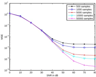
Figure 5 and Table I shortly illustrate the validity of the third separation method (virtual meas. + ICA) in the case when the mixture is given by (18). Figure 5 shows the MSE obtained on the reconstructed sources (before elimination of residual noise with a hard decision) and Table I gives the Bit Error Rate (BER) (after applying a sign function). All values have been obtained by averaging on 1000 Monte-Carlo runs. One can notice that in low noise conditions, the nonlinear mixture is perfectly inverted.
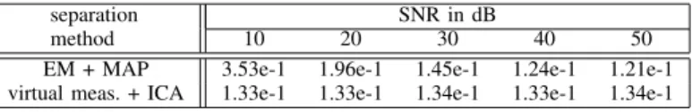
Tables II and III compare the three separation methods de-scribed above. One can see in Table II that resorting to MAP estimation gives better results than using the exact inversion formula: this is no surprise since the exact inverse is only valid in the noiseless case. However, the method considering virtual measurements outperforms the classification by MAP: this is actually due to the difficulty of initializing the EM algorithm which may get trapped in a local maximum [17]. If a good initialization point was given to the EM algorithm, the EM + MAP separation method would outperform all the other ones. Note also that these results are not specific to the mixture (18). According to the simulations in Table II, they remain when the mixture is given by (9) with randomly generated parameters
a, b, c, d. Finally, another advantage of the proposed method of
virtual measurements is illustrated in Table III where one can see that the execution time is constant. Again, this advantage is due to the difficulty of initializing the EM algorithm: if badly initialized, it may converge slowly or even require a new initialization step.
It follows from these observations that the proposed method is complementary to the (EM + MAP) classification and one can hence think about combining both in order to improve the quality of the result: one apparently attrative solution consists in using the result given by (virtual meas. + ICA) as an ini-tialization point to the (EM + MAP) method. This has been tried and results are given on the line indicated by ICA + EM + MAP in Table II.
VII. CONCLUSION
In this paper, we have illustrated that algebraic methods constitute powerful methods to deal with the particular class of polynomial MIMO systems. They offer an attractive answer to the problem of their inversion. Many interesting signals, such as telecommunication ones, admit a finite number of values: in this case, the former tools show that there is more flexibility concerning inversion. In addition, we have shown that there exist a linear model which is equivalent to the original nonlinear one. In a blind context, this equivalent linear model suffers from the problem of underdetermination and of dependency between virtual sources. Finally, we have applied our result to the problem of blind separation of two binary sources mixed nonlinearly: based on the specificity of these sources, and although the virtual sources of the equivalent model are not independent, classical ICA algorithms succeed to separate the virtual sources.
APPENDIXI PROOF OFPROPERTY2
Proof: For any ideal I and for the polynomial with distinct roots q1(s1) = Ql1 k=1 ³ s1− ˜a(k)1 ´ , we have [16, p.45] (see Definition 5 for the sum of two ideals):
I + hq1i = l1 \ k1=1 ³ I + hs1− ˜a(k11)i ´
It follows that we can write:
hq1, . . . , qNi = hq2, . . . , qNi + hq1i =\ k1 ³ hq2, . . . , qNi + hs1− ˜a(k11)i ´
and decomposing similarly hq2, . . . , qNi + hs1− ˜a(k11)i:
hq1, . . . , qNi = \ k1k2 ³ hq3, . . . , qNi + hs1− ˜a1(k1), s2− ˜a(k22)i ´
Il we repeat further this operation, we finally obtain:
hq1, . . . , qNi =
\
k1...kN
hs1− ˜a(k11), . . . , sN − ˜a(kNN)i = IA
Finally, to prove that {q1, . . . , qN} is a Groebner basis,
observe that the qi are univariate polynomials. Their terms
are hence ordered independently of the ordering ≺ on K[s] and their leading terms are sl1
1, . . . , slNN respectively. One can
then check that these polynomials satisfy the criterion on the S-polynomials [15, p.82] for {q1, . . . , qN} to be a Groebner
basis. Finally, one can verify that {q1, . . . , qN} is indeed a
APPENDIXII
PROOF OFPROPOSITION1
Proof: The proof is very similar to the proof of Theorem
2 in [15, p.334].
Choose q1, . . . , qP in K[s] such that IA= hq1, . . . , qPi and
let I = IA+ hf1− x1, . . . , fQ − xQi = hq1, . . . , qP, f1−
x1, . . . , fQ− xQi. If g is the remainder of h on division by
the Groebner basis G of I, we can write:
h = B1(s, x)(f1− x1) + · · · + BQ(s, x)(fQ− xQ)
+ C1(s, x)q1+ · · · + CP(s, x)qP+ g
where B1, . . . , BQ, C1, . . . , CP are in K[s, x]. If g ∈ K[x],
substituting fi for xi in the above expression, we obtain:
h = C1(s, f )q1+ . . . CP(s, f )qP+ g(f1, . . . , fQ)
and thus with r = C1(s, f )q1+ . . . CP(s, f )qP ∈ IA, we have
h − r = g(f1, . . . , fQ) ∈ K[f ]
Conversely, assume there is r ∈ IAsuch that h − r ∈ K[f ].
Then we can write h − r = ˜g(f1, . . . , fQ) for a polynomial ˜g
in K[x]. Similarly to [15, p.315, Eq. (4)], we can write: ˜
g(f1, . . . , fQ) = ˜g(x1, . . . , xQ)+E1(f1−x1)+· · ·+EQ(fQ−xQ)
where E1, . . . , EQ are in K[s, x]. Then:
h = ˜g(x1, . . . , xQ) + E1(f1− x1) + · · · + EQ(fQ− xQ) + r
Now let G0 = G ∩ K[x] and ˜˜g be the remainder of the
division of ˜g by G0. We have then: h = h
I+ ˜˜g + r, where
hI∈ I.
Relying on the elimination property of the ordering, we can use the same arguments as in [15, p.335] to prove that ˜˜g is
the remainder of division of h by G. Hence we have ˜˜g = g,
which proves that g ∈ K[x].
The second part of the proposition follows from the above arguments.
APPENDIXIII
IMPLEMENTATION OF THE PROVIDED EXAMPLES
In this appendix, we show how the results in the paper are obtained using a computer algebra system. We used SINGU
-LAR [27] which is a software freely available on the web.
A. Example from Section IV-A
The ring should first be defined, and then the polynomials corresponding to Equation (5): ring r=0,(s1,s2,x1,x2,x3,x4),lp; poly f1= 3*s1ˆ2+2*s1*s2+4*s2ˆ2+7*s1+4*s2; poly f2=-3*s1ˆ2+5*s1*s2+2*s1+s2; poly f3=-3*s1+6*s2; poly f4=6*s1ˆ2-s1*s2+4*s2ˆ2+3*s1-9*s2; The following lines define the ideal I, compute its Groebner basis (denoted G1) and perform the division of s1, s2 by G1:
ideal I1=f1-x1,f2-x2,f3-x3,f4-x4; ideal G1=groebner(I1);
reduce(s1,G1); reduce(s2,G1);
B. Example from Section IV-B
The following lines show that s1, s2cannot be recovered from
x1, x2, x3 only:
ideal I2=f1-x1,f2-x2,f3-x3; ideal G2=groebner(I2);
reduce(s1,G2); reduce(s2,G2);
We then test the algebraic dependence between f1, f2, f3 :
LIB "algebra.lib";
algDependent(ideal(f1,f2,f3))[1];
The example in Section IV-B is then obtained by computing in the ring denoted r2:
ring r2=(0,b1,b2),(s1,s2,x1,x2,x3,x4),lp; ideal G2=imap(r,G2);
reduce((s1ˆ2+b1*s1),G2); reduce((s2ˆ2+b2*s2),G2);
C. Example from Section V-B
The only difference in the case of finite alphabet sources is that we should enter and define the ring IA (The first line
switches back to the working ring denoted r since we defined r2 above). setring r; ideal Ia= (s1-1/2)*(s1-3/2)*(s1+1/2)*(s1+3/2), (s2-1/2)*(s2-3/2)*(s2+1/2)*(s2+3/2); ideal I3=f1-x1,f2-x2,f3-x3,Ia; ideal G3=groebner(I3); reduce(s1,G3); reduce(s2,G3);
D. Example how to derive Equation (17)
ring r3=(0,a,b,c,d),(s1,s2,x),lp; ideal I4=a*s1*s2+b*s1+c*s2+d-x,s1ˆ2-1, s2ˆ2-1; ideal G4=groebner(I4); reduce(s1,G4); reduce(s2,G4); REFERENCES
[1] S. Achard and C. Jutten. Identifiability of post-nonlinear mixtures. IEEE
Signal Processing Letters, 12(5):423–426, May 2005.
[2] H. Arfa, S. E. Asmi, and S. Belghith. A nonlinear channel equalization using an algebraic approach and the affine projection algorithm. In
European Signal Processing Conference (EUSIPCO), Florence, Italy,
September 2006.
[3] S. E. Asmi and M. Mboup. On the equalizability of nonlinear/time-varying multi-user channels. In Proc. IEEE Int. Conf. on Acoustics,
Speech and Signal Processing (ICASSP), volume 4, pages 2133–2136,
May 2001.
[4] M. Babaie-Zadeh. On blind source separation in convolutive and nonlinear mixtures. PhD thesis, INP of Grenoble, France, 2002.
[5] M. Babaie-Zadeh and C. Jutten. A general approach for mutual information minimization and its application to blind source separation.
Signal Processing, 85(5):975–995, May 2005.
[6] M. Babaie-Zadeh, C. Jutten, and K. Nayebi. Blind separating convolutive post non-linear mixtures. In Proc. of ICA’01, pages 138–143, San Diego, December 2001.
[7] A. J. Bell and T. J. Sejnowski. An information-maximisation approach to blind separation and blind deconvolution. Neural computation,