HAL Id: hal-00451950
https://hal.archives-ouvertes.fr/hal-00451950
Submitted on 26 Jun 2019
HAL is a multi-disciplinary open access
archive for the deposit and dissemination of
sci-entific research documents, whether they are
pub-lished or not. The documents may come from
teaching and research institutions in France or
abroad, or from public or private research centers.
L’archive ouverte pluridisciplinaire HAL, est
destinée au dépôt et à la diffusion de documents
scientifiques de niveau recherche, publiés ou non,
émanant des établissements d’enseignement et de
recherche français ou étrangers, des laboratoires
publics ou privés.
Static and Dynamic Analysis of the PAMINSA
Vigen Arakelian, Sylvain Guegan, Sébastien Briot
To cite this version:
Vigen Arakelian, Sylvain Guegan, Sébastien Briot. Static and Dynamic Analysis of the PAMINSA.
IDETC/CIE, ASME 2005 International Design Engineering Technical Conferences & Computers and
Information in Engineering Conference, Sep 2005, Long Beach, CA, United States. pp.803-809,
�10.1115/DETC2005-84679�. �hal-00451950�
STATIC AND DYNAMIC ANALYSIS OF THE PAMINSA
(Parallel Manipulator of the I.N.S.A.)
Vigen Arakelian Sylvain Guégan Sébastien Briot
Département de Génie Mécanique et Automatique - L.G.C.G.M. EA3913 Institut National des Sciences Appliquées (I.N.S.A.)
20 avenue des Buttes de Coësmes – CS 14315 F-35043 Rennes, France
Email : [email protected]
KEYWORDS: Parallel manipulator, decoupled motions, static optimization, dynamic modeling
ABSTRACT
In this paper we present an analytical approach for the static and dynamic analysis of the PAMINSA1, a new 4 degrees of freedom parallel manipulator that has been designed at the I.N.S.A.2 in Rennes. On the base of the developed static model, the input torques due to the static loads are reduced by means of the optimum redistribution of the moving link masses. The analytical dynamic modeling of the PAMINSA by means of Lagrange equations is achieved. A numerical example and a comparison between the suggested analytical model and an ADAMS software simulation are presented.
INTRODUCTION
The complex nonlinear dynamics appears to be one of the most important parallel manipulator characteristics. Even in the static model, the expression of the torques (or forces) applied to the actuators due to the weight of the platform and links, are nonlinear. Driving torques on parallel manipulators are highly nonlinear functions of the position, velocity and acceleration of the mechanical actuator links. It should be noted that there are algorithms to regulate the problems of non-linearity (static or dynamic) and to ensure an efficient control and an acceptable computation cost. However, the simplification of the manipulator mechanical model is desirable and a mechanical
1 Parallel Manipulator of the I.N.S.A.
2 Institut National des Sciences Appliquées (I.N.S.A.) – National Institute of Applied Sciences.
system with a linear input/output relation is more appealing for industrial applications.
In the recent years, the decoupling of motions of parallel manipulators has attracted researchers’ attention and different structures have been proposed [1-8]. Previous works on this problem may be arranged into two principal groups: (a) fully decoupled parallel structures in which the architecture of the manipulator is such that its input/output equations are linear and fully decoupled [1-5]; (b) position/orientation decoupled manipulators in which the end-effector’s position is independent of the orientation [6-8].
Another trend of the kinematic decoupling is proposed in the design of the PAMINSA3. It consists in decoupling the motions in the horizontal plane and the translation along the vertical axis.
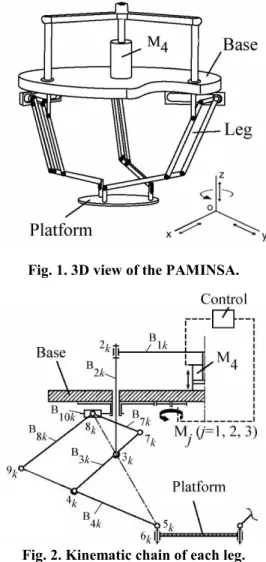
DESCRIPTION OF THE PAMINSA
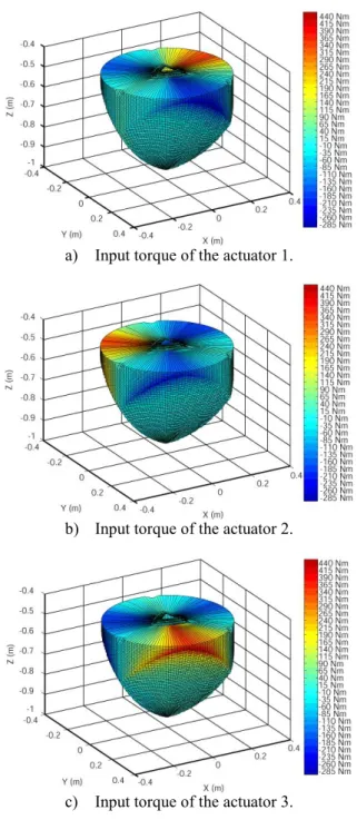
Fig. 1 shows a 3D model of the PAMINSA with three legs. Each leg of the manipulator is realized by a pantograph mecha-nism (Fig. 2) with two input points 3k and 8k, and an output
point 5k (k = 1, 2, 3). Each input point 8k is connected with the
rotating drive Mi by means of the prismatic guide mounted on
the rotating link. This type of manipulator architecture allows the generation of motion in the horizontal plane by the rotating actuators M1, M2, M3 and the vertical displacements by the linear actuator M4. Thus the displacements (x, y, ) of the platform in the horizontal plane (xOy) are independent of the vertical displacements z.
3 Patent concerning the PAMINSA is pending and a prototype is currently being developed.
In the concept of the PAMINSA, the following properties of the hand operated manipulators [9,10] are used: the work of the gravitational forces of the manipulated object displaced in the horizontal plane is zero because the gravitational forces are always perpendicular to the displacements. However, the work of the same forces in the case of the vertical displacements is different from zero (the gravitational forces are parallel to the displacements).
Thus, the rotating actuators move the platform in the horizontal plane and their work due to the gravity of the manipulated object is equal to zero.
Fig. 1. 3D view of the PAMINSA.
Fig. 2. Kinematic chain of each leg.
The obvious advantages of the PAMINSA are the following:
a) the decoupling of the drive powers into two groups, which allows the lifting of heavy load to a given altitude with only one very powerful actuator and then, by using other less powerful actuators, its accurate positioning in the horizontal plane, i.e. it is possible to use two kinds of actuators;
b) a simplification of the vertical control based on the linear input/output equation (vertical displacements of the platform and the linear actuator are copied by a magnification factor);
c) the improvement of positioning accuracy along the vertical axis because the mechanical locking of the structure does
not allow the altitude variations during the displacements in the horizontal plane;
d) the improvement of positioning accuracy in the horizontal plane because the loads on the rotating actuators Mj due to
the gravitational forces of the platform are cancelled. It appears to us that the proposed manipulator could be used in industrial applications for the manipulation of heavy equipments with great positioning accuracy. Various fields are possible depending on the type of the industrial application.
This contribution deals with the static and dynamic analysis of the PAMINSA. The obtained results will be used for the optimization of the dynamic behaviour of a prototype, which is currently being developed at the I.N.S.A.
STATIC ANALYSIS AND INPUT TORQUES OPTIMIZATION
The torques (or forces) Qj applied to the actuators Mj (j = 1,
2, 3, 4) due to the force of gravity of links, joints and platform of the studied manipulator can be expressed as:
, ( 1,2,3,4) 3 1 1
j Q Q Q k n i st ikj st plj st j , (1) where st ikjQ is the load applied to the actuator j due to the
gravity of the i-th link or bearings of the k-th leg (k = 1, 2, 3),
st plj
Q is the load applied to the actuator j due to the gravity of
the platform.
These loads can be represented in the form: j k ik T ik st ikj x y z x y z Q
3 1 ) , , , ( ) , , , ( J G (2)
T pl
j plj Q J G , (3) where Jik is the Jacobian matrix between the point Pik and theactuated variables qj, Pik is the center of masses of the i-th link,
J is the general Jacobian matrix of the robot, between the point P and the actuated variables qj, P is the center of masses of the
platform, G and Gik are respectively the forces of gravity of the
platform and the links (or bearings). It is easy to see that:
T pl
j pljQ J G =0, for j = 1, 2, 3. (4) i.e. the input torques of the rotating actuators due to the gravity of the platform are cancelled because the gravitational forces are always perpendicular to the displacements (the platform carry out the displacements in the horizontal plane).
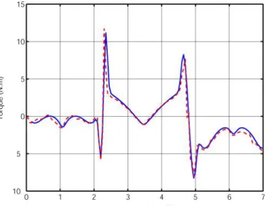
Fig. 3 shows the redistribution of the actuator input torques for the whole workspace of the PAMINSA (for = /3, where
is the rotation angle of the platform about the z axis). The values of the input torques are differentiated by the different colors.
It should be noted that the workspace of the PAMINSA is symmetrical and the maximum values of the input torques are the same for all actuators but they are situated in different zones.
a) Input torque of the actuator 1.
b) Input torque of the actuator 2.
c) Input torque of the actuator 3. Fig. 3. Actuator input torques.
Thus, the input torques of the rotating actuators are the following: ), 3 , 2 , 1 ( , ) , , , ( 3 1 1
j z y x Q Q k n i st ikj st j (5) where j k ik T ik st ikj x y x y z Q
3 1 ) , , , ( ) , , ( J G . (6)In the work [10], it was shown that the input torques st j Q of
the pantograph linkage can be cancelled by optimal redistribution of movable masses.
Thus, in the same way as in the work [10] we can obtain:
Qpljst 0, (j1,2,3), (7)
and consequently
Qjst 0, (j1,2,3), (8)
In conclusion one can note the input torques of the rotating actuators M1, M2 and M3 due to the gravity are completely eliminated and the displacements of the platform in the horizontal plane may be realized without great efforts (the residual efforts are due to the resistance due to the friction in the joints and the errors due to the elasticity of the links). DYNAMIC ANALYSIS
The analytical model for dynamics of the PAMINSA based on the Lagrange equations has been formulated to compute the input torques which are necessary to control a given trajectory of the movable platform. In order to simplify the mathematical model, the effects of link elasticity and the friction in the joints have been neglected. The pantograph linkages are assumed to be composed of rigid bodies connected by joints without inner clearance.
It should be noted that a CAD model of the studied manipulator has been developed and more real simulation could be carried out on the software ADAMS.
The studied manipulator has 4 degrees of freedom, so it is natural to select the 4 joint variables
1,2,3,Z
as the 4generalized coordinates, and then evaluate a set of 4 Lagrange equations for these coordinates. Such equations would be the formulas for the unknown torques (or forces).
However, due to the complexity of the geometrical model, the evaluation of the Lagrange function and especially its derivatives with four coordinates only, is found to be extremely involved. So we use the same approach as in the study [11] and we increase the number of the generalized coordinates.
In this studied case, it is better to choose the following 8 generalized coordinates:
qj
x,y,,z,1,2,3,Z
, j =1, …, 8 (9)The notation used to describe the pantograph linkages is included below: (fig. 2)
Bik the link between the joints i and i+1 on the leg k
mi the mass of i-th joint
mBi the mass of the link Bik
lBi the length of the link Bik
i
I the inertia matrix of the link Bik
We consider that the links are perfect tubes, i.e.
) ( ) ( ) ( 0 0 0 0 0 0 i ZZ i YY i XX i I I I I , with IYY(i)IZZ(i) (10)
Potential Energy
The potential energy V of the manipulator can be expressed as follow:
3 1 k leg pl V k V V (11) where, z g mVpl pl is the potential energy of the platform,
3 3 9 2 5 1 z M z M Z e M Vleg p k p k p k is the potential
energy of the leg k,
g is the gravitational acceleration,
the expression of z5k and z9k are given in Appendix 1 and the expression of Mpi, (i = 1, 2, 3) and e3 are given in Appendix 2. Kinetic Energy
The kinetic energy T of the manipulator can be represented in the form:
3 1 k leg pl T k T T , (12) where,
( 2 2 2) 2
2 1 pl pl pl m x y z IT is the kinetic energy of
the platform, k k k trans rot
leg T T
T is the kinetic energy of the leg k,
2 8 5 7 6 9 5 5 9 5 9 5 4 2 9 2 9 2 9 3 2 5 2 2 5 2 5 1 ) ( ) ( ) ( k c k c c k k c k k k k c k k k c k c k k c trans M Z z M Z M z z M y y x x M z y x M z M y x M T k (13) k rot
T is the kinetic energy of the rotating links.
Let us note that there are two types of rotations (Fig. 4): - rotation due to the actuators Mj (j=1, 2, 3) (angle k),
which is about of the vertical axis,
- rotation due to the displacement of the pantograph in the linkage plane (angles k and k).
Fig. 4. A scheme for representation of the rotations of the k-th pantograph linkage.
The kinetic energy of the rotating links can be written as:
)) ( cos ) ( sin ) ( cos ) ( sin ( 2 11 2 12 2 9 2 10 13 2 2 10 2 9 k c k c k c k c c k k c k c rot M M M M M M M T k (14)
The expressions for Mci (i = 1, …, 13) are given in
Appendix 3.
So the Lagrange function of the system is given by the formula LTV and the Lagrange equations are the following:
4 1 d d i ij i j j j A Q q L q L t . (15) wherei are the Lagrange multipliers (i=1, …, 4),
qj are the generalized coordinates (j=1, …, 8),
Qj are the input torques or forces.
Coefficients Aij are obtained by differentiating the
closure-loop equations of the manipulator with respect to the generalized coordinates. These equations are given by the expressions: 0 ) cos( ) ( ) sin( ) ( 5 1 5 2 k k k k k k k x e y e s
, k=1, 2, 3 (16) 4 5 20 C k Z lC k l z s . (17)The expressions for k, e1k and e2k are given in Appendix 1. The system of equations (15) is solved as follow: firstly the Lagrange multipliers must be obtained from the first four Lagrange equations (for qj x,y,,z) and then the input
torques/forces can be determined from the last four Lagrange equations: 15 1 1 1 5 d d A L L t Q (18) 26 2 2 2 6 d d A L L t Q (19) 37 3 3 3 7 d d A L L t Q (20) 48 4 8 d d A Z L Z L t Q (21) NUMERICAL SIMULATIONS
In order to verify the obtained expressions for the dynamic model of the PAMINSA, we compared a numerical application of the analytical computation with the ADAMS software simulations. For this purpose a CAD model of the PAMINSA (Fig. 5) has been developed with the parameters given in Appendix 4.
The variation of the input torques/forces for the prescribed trajectory (Appendix 5 - Fig. 8 to 11) with 1m/s² maximal acceleration has been computed and compared with the ADAMS simulations. The variation of the input torque of the rotating actuator 1 and the input effort of the linear actuator 4 for the entirely analytic dynamic model and the ADAMS simulation are shown in Fig. 6 and Fig. 7. The values of the input torques are differentiated by the different colors. The blue
continuous curve represents the results of the analytic model and the red dotted curve the ADAMS simulation.
The obtained results show that the examined functions are identical. The small differences between the analytic dynamic model and the ADAMS simulation are probably caused by numerical noise.
Thus, the analytical dynamic model of the PAMINSA is validated and can be implemented to improve the performance of the control by taking into account, partially or totally all the dynamic interaction torques.
Fig. 5. CAD model of the PAMINSA.
CONCLUSIONS
Static and dynamic analysis of the new parallel manipulator with 4 degrees of freedom, called the PAMINSA has been presented. By using an optimal redistribution of masses of the pantograph linkages, the input torques of the rotating actuators of the PAMINSA are cancelled. An analytical model based on the Lagrange equations was formulated and a simplified approach for its solution was proposed. Results of numerical simulations have been presented to show the feasibility of the proposed analytical approach.
Fig. 6. Comparison of the Lagrange dynamic model and ADAMS simulation for the input torque of the actuator 1.
Fig. 7. Comparison of the Lagrange dynamic model and ADAMS simulation for the input force of the actuator 4.
REFERENCES
[1] Kong, X. and Gosselin, C. M., 2002, “A class of 3-dof translational parallel manipulator with linear input/output equations”, Workshop on Fundamental Issues and Future Research for Parallel Mechanisms and Manipulators, Québec City, Québec, Canada, pp. 25–32.
[2] Gosselin, C. M., Kong, X., Foucault, S. and Bonev, I. A., 2004, “A fully decoupled 3-dof translational parallel mechanism”, Parallel Kinematic Machines International Conference, Chemnitz, Germany, pp. 595–610.
[3] Carricato, M. and Parenti-Castelli, V., 2004, “A novel fully decoupled 2-dof parallel wrist”, The International Journal of Robotics Research, 23(6), pp. 661–667.
[4] Carricato, M. and Parenti-Castelli, V., 2004, “On the topological and geometrical synthesis and classification of translational parallel mechanisms”, Proc. of the 11th World Congress in Mechanism and Machine Science, Tianjin, China, pp. 1624–1628.
[5] Bouzgarrou, B. C., Fauroux, J. C., Gogu, G., and Heerah, Y., 2004, “Rigidity analysis of T3R1 parallel robot with uncoupled kinematics”, International Symposium on Robotics, Paris, France.
[6] Patarinski, S.P. and Uchiyama, M., 1994, “Analysis and design of position/orientation decoupled parallel manipulator”, Proc. of Romansy, Theory and practice of robots and manipulators, 10th CISM IFTOMM Symposium, 9, pp. 1-6. [7] Patarinski, S.P. and Uchiyama, M., 1993, “Position/orientation decoupled parallel manipulators”, ICAR, Tokyo, Japan, pp. 153-158.
[8] Lallemand, J.P., Goudali, A. and Zeghloul, S., 1997, “The 6-dof 2-Delta parallel manipulator”, Robotica, 15, pp. 407-416. [9] Arakelian, V., 2004, “The history of the creation and development of hand-operated balanced manipulators”, Proc. HMM2004, Kluwer Academic Publishers
[10] Arakelian, V., 1998, “Equilibrage des manipulateurs manuels”, Mechanism and Machine Theory, 33(4).
[11] Miller, K. and Clavel, R., 1992, “The lagrange-based model of delta-4 robot dynamics”, Robotersysteme, 8, pp. 49-54.
APPENDIX Appendix 1 5 51 51 51 51 sin( /6) ) 6 / cos( B pl pl l z R y R x z y x P 5 52 52 52 52 sin( /6) ) 6 / cos( B pl pl l z R y R x z y x P 5 53 53 53 53 cos sin B pl pl l z R y R x z y x P
where Rpl is the platform radius.
b R e e 2 3 12 11 , 2 22 21 b R e e , e310 and e32Rb,
where Rb is the base radius.
6 / 1 1 , 225/6, 333/2 F H e H e z y x k k k k k k k k sin( ) ) cos( 2 1 9 9 9 9 P where: F B A H , F(DK)/(2E), K D24EC, ) 1 ( 2 B E , D2B(X4A), 2 4 2 4 2 3 X 2 A X A l C B , BZ1/(kX4), ) 2 /( ) (l24 l23 X12 X42 Z12 k X4 A B B , Z1z5k, ) 1 /( 1 4X k X and X1 (x5ke1k)2(y5ke2k)2 . Appendix 2
2,3,4,7 1,7 3 2 4 5 1 2 2 i i i Bi Bi B i p k m k m m k m m g M 2 2 ) 2 ( ) 1 ( 8 4 7 3 9 7 4 2 B B B B p m m k m m k k m k m m k g M 2 1 3 B p m g M , 2 2 1 2 2 3 B B B m m m l g e Appendix 3 2 8 2 2 7 4 2 2 3 2 8 2 7 5 2 4 1 )) 1 ( 2 ( )) 1 ( 2 ( ) 1 ( 4 )) 1 ( 2 ( ) 2 ( ) 1 ( )) 1 ( ( 2 1 k m k k k m m k k k m k m k k m m k m M B B B B c
4 4 2 1 3 4 2 2 7 , 1 2 5 7 , 4 , 3 , 2 2 2 B i Bi i Bi i i c m k m k m m k m M 4 4 4 4 ) 2 ( ) 1 ( 2 1 8 2 7 4 2 2 3 9 2 7 2 4 2 3 B B B B c m k m m k k m m k m k m k M ) 1 ( 2 ) 1 ( 2 ) 1 ( 2 ) 1 ( 2 ) 2 ( ) 1 ( ) 1 ( 2 2 1 8 2 7 4 2 2 3 2 7 2 4 4 k m k k k m m k k k m k k m k m k M B B B B c 2 2 ) 2 ( 2 ) ) 1 (( 4 2 1 4 2 3 7 7 4 5 B B B c m k k m m m m k M 8 1 6 B c m M , k m Mc B 4 1 7 , 8 2 10 10 8 B B c l m M , 2 ) 7 ( ) 4 ( 9 B YY B YY c I I M , 2 ) 7 ( ) 4 ( 10 B XX B XX c I I M , 2 ) 8 ( ) 3 ( 11 B YY B YY c I I M , 2 ) 8 ( ) 3 ( 12 B XX B XX c I I M , 2 10 2 13 B B c I I M g=9.81m/s² Appendix 4 k=3, Rb=0.35m, Rpl=0.1m lB1=0.308m, lB2=0.442m, lB3= lC8=0.42m, lB4=k lB7=0.63m, lB5=0.0275m, lB10=0.3635m m2=0.214kg, m3=0.338kg, m4=0.262kg, m5=0.233kg, m7=0.28kg, m8=0.305kg, m9=0.259kg, mpl=2.301kg, mB1=1.221kg, mB2=0.921kg, mB3=0.406kg, mB4=0.672kg, mB7=0.107kg, mB8=0.403kg, mB10=0.436kg. 2 ) 3 ( kg/m 0038 . 0 B XX I , 2 ) 3 ( kg/m 02 . 0 B YY I , 2 ) 4 ( kg/m 0012 . 0 B XX I , 2 ) 4 ( kg/m 048 . 0 B YY I , 2 4 ) 7 ( kg/m 10 8 B XX I , 2 ) 7 ( kg/m 003 . 0 B YY I , 2 ) 8 ( kg/m 0024 . 0 B XX I , 2 ) 8 (B 0.02kg/m YY I , 2 20.003kg/m B I , 2 100.02kg/m B I and Ipl0.015kg/m2.Appendix 5: Trajectory used for the simulations
Fig. 8. Position of the moving platform about x axis.
Fig. 9. Position of the moving platform about y axis.
Fig. 10. Position of the moving platform about z axis.