Tarification et aide à la décision avec effets de prix de référence

(1)

Faculté des Sciences, 4 Avenue Ibn Battouta B.P. 1014 RP, Rabat, Tél : + 212 (0) 5 37 77 18 34/35/38, http://http://www.fsr.um5a.ac.m a/ UNIVERSITÉ MOHAMMED V – AGDAL

FACULTÉ DES SCIENCES RABAT N°d’ordre : 2723 THÈSE DE DOCTORAT Présentée par Youssef OUMANAR Discipline: Mathématiques Spécialité: Recherche Opérationnelle

Tarification et Aide à la Décision avec

Effets de Prix de Référence

Soutenue le: 19 juillet 2014, devant le jury:

Président:

M. Hassan Hbid Professeur à la Faculté des Sciences Semlalia de Marrakech Examinateurs:

Mme Noha El Khattabi Professeur à la Faculté des Sciences de Rabat M. Jilali Mikram Professeur à la Faculté des Sciences de Rabat

Mme Rajaa Aboulaich Professeur à l’École Mohammadia d’Ingénieurs à Rabat M. Slimane Ben Miled Professeur à la Faculté des Sciences de Tunis

Encadrants :

Mme Nadia Raissi Professeur à la Faculté des Sciences de Rabat M. Soulaymane Kachani Professeur à Columbia University à New York Invités:

(2)

(3)

ACKNOWLEDGMENTS

The work presented in this thesis was performed at the "Laboratoire d’Analyse, Algèbre et Aide à la décision" at the Faculty of Science of Rabat.

I have benefited greatly from the support, guidance, and love of many people throughout the years of preparation of this thesis.

First and foremost, I would like to express a deep sense of thanks and gratitude to my doctoral supervisors, Nadia Raissi and Soulaymane Kachani. Nadia Raissi was also my Master’s thesis supervisor. She has always placed her trust in me, oﬀered me unparalleled opportunities, and encouraged me to go the extra mile. Beyond the academic level, Nadia Raissi is a wonderful person who genuinely cares for all her students. She gets involved in so many ways to oﬀer them a better situation to conduct their research and to thrive in life. Soulaymane Kachani is the kind of person that one meets once in a lifetime. I have learned so much from him. I am greatly indebted to him for his insight and valuable supervision. Completion of this PhD would not have been possible without his support and guidance.

I would also like to extend a sincere thank you to Mr. Hassan HBID, Professor and Dean of the Faculty of Science Semlalia, for being the Jury President of my PhD examination committee and to thank Mrs. Noha El KHATTABI, Professor at the Faculty of Science in Rabat, and Mr. Slimane BEN MILED, Professor at the Faculty of Science in Tunis, for taking the time to issue reports on my thesis. I owe a thank you to the rest of the Jury members, Mr. Jilali MIKRAM, Professor and Chair of the Math Department at the Faculty of Science in Rabat, and Mrs. Rajaa ABOULAICH, Professor at Mohammadia Engineering School, for oﬀering their valuable time to read my thesis and for accepting to attend my defense in Rabat.

May I express here the gratitude I feel toward the members of the Moroccan-American Commission for Educational & Cultural Exchange (MACECE), particularly Dr. James Miller and Mr. Mohammed Chrayah, for believing in me and funding my stay in the United States as a Fulbright Scholar.

I benefited immensly from the intense research atmosphere at Columbia Univer-sity and at the department of Industrial Engineering and Operations Research in particular. I would like to pay tribute to the faculty and student body with which I had invaluable interactions.

(4)

ii

Amine Chater, Jimmy Taylor, Morton Berenbaum, Gil Perez, and Mary Murphy, for their support at all times and for making my stay in the United States enjoyable. May they find here my sincere appreciation.

I would also like to express my heartfelt gratitude to my wife, Jodhy, for her pa-tience and support during my work on this dissertation. Her presence in diﬃcult times was of inestimable value.

Finally, I am eternally grateful to my family for their unconditional love and support. I would like to pay special mention and tribute to my parents and my grandmother, Oumkeltoum El Bied, for their continuous support, the importance they have always placed on my education, and their belief in my ability to succeed. I will remain indebted to them forever and I dedicate this thesis to them.

(5)

iii

Résumé:

Dans cette thèse, nous développons des modèles de pricing dynamique pour des commerçants qui vendent des produits à un flux de clients répétitifs sur un horizon infini. Ces modèles comprennent le concept de prix de référence tant au niveau du produit qu’au niveau du magasin. Nos modèles sont présentés dans un contexte d’un commerce de détail mais ont pour but de capturer une application plus générale et d’être implémentés dans diﬀérrentes industries telles que le transport aérien, l’hôtellerie, la restauration ou encore la location de voitures.

Depuis une dizaine d’années, les techniques de Revenue Management ont été développées d’une manière extensive par les compagnies aériennes et les hôtels. Une grande partie de la recherche a porté sur le front de l’optimisation qui consiste à détrminer la politique optimale d’allocation de la capacité afin de maximiser le revenue. Bien que les prévisions économiques constituent la pierre angulaire de tout système de Yield Management réussi, il y a eu moins de publications relevants de leur développement. Il est important de noter que la qualité des prévisions a un impact direct sur celle des stratégies de tarification et d’allocation de capacité ainsi que sur d’autres pratiques comme la surréservation. Dans un premier temps, nous utilisons diﬀérentes méthodes de prévision et comparons leur performance en nous basant sur des données de réservation réelles d’un hôtel.

Dans une seconde partie, nous nous concentrons sur la composante de pricing et nous dérivons une solution analytique pour la politique optimale de pricing dans un marché de monopole. Notre stratégie optimale de tarification est une fonction de la condition actuelle du marché, representée par le prix de référence, contrairement aux travaux précédents où la politique de pricing est une fonction du temps. Nous prouvons la convergence monotone des prix optimaux et des prix de référence à leurs états d’équilibre réspectifs.

Dans une troisième partie, nous proposons un modèle dynamique de pricing, pour un commerçant vendant multiple produits, basé sur la notion du prix de référence du magasin. Nous dérivons une politique optimale de pricing et prouvons sa convergence monotone dans un contexte de monopole. Nous dérivons une forme analytique pour les prix optimaux. De plus, nous dressons une comparaison entre les modèles établis au niveau du magasin et ceux établis au niveau des produits et entre les politiques optimales et myopes.

(6)

iv

Enfin, dans la quatrième partie, nous considérons un marché de duopole où les commerçants rivalisent à travers les dynamiques de prix de référence au niveau du magasin. Nous dérivons un système d’équations qui peut être facilement résolu numériquement pour un équilibre de Markov parfait. Nous proposons une heuristique et démontrons que son résultat est très proche de l’équilibre. De plus, nous dérivons des solutions analytiques à des problèmes de pricing pour un commerçant quand son compétiteur suit l’une de trois stratégies sous-optimales et on prouve la convergence monotone des solutions. Pour conclure, on utilise nos résultats pour analyser l’impact de la compétition en comparant le revenue de la politique optimale avec et sans compétition. Mots clés : Prix de référence, tarification, méthodes de prévisions économiques, com-portement des acheteurs, aide à la décision, optimisation dynamique, stratégies compéti-tives, théorie des jeux.

(7)

v

Abstract:

In this thesis, we develop dynamic pricing models for retailers selling multiple products to a stream of repeated customers over an infinite time horizon. These models incorporates the concept of a reference price both at the product level and the store level. Our models are presented in the context of a retailer but they are aimed to capture a broader application and to be implemented in several businesses such as the airline industry, hotel industry, restaurant businesses or car rentals.

Over the past decade, revenue management techniques have been extensively developed in the airline and hotel industries. Much of the research has been on the optimization front, which focuses on finding the optimal seat allocation policy to maximize revenue. Although forecasting lies in the heart of every successful revenue management operation, there has been less published work on its issues. It is important to note that the quality of the forecasting is instrumental in deriving robust and reliable pricing/room allocation decisions and other practices such as overbooking. In the first part of this thesis, we utilize various forecasting techniques and compare their performance based on real-life hotel booking data.

In the second part of this thesis, we focus on the pricing component and we derive a closed-form solution for the optimal pricing policy in a monopoly market. Our optimal pricing policy is a function of the current market condition, represented by the reference price, as opposed to the previous works where the pricing policy is a function of time. We prove the monotone convergence of the optimal prices and the store’s level reference price to their respective steady states.

In the third part of this thesis, we propose a dynamic pricing model, for a retailer selling multiple products, based on the notion of store-level reference price. We derive an optimal pricing policy and prove its monotone convergence in a monopoly context. We derive an analytical result for the optimal prices. Also, we address a comparison between the store-level and the product-level models and between optimal and myopic policies. Finally, in the fourth part of this thesis, we consider a Duopoly market where firms compete through dynamics of the reference price on their store’s price level. We derive a system of equations that can be easily solved numerically for a Markov-Perfect Equilibrium pricing policy. We provide a closed-form heuristic and demonstrate that

(8)

vi

it is very close to the equilibrium. We also derive closed-form solutions for pricing policies of a retailer who is an optimizer when its competitor follows one of three diﬀerent suboptimal policies, and prove monotone convergence of these solutions. And to conclude, we use our results to analyze the impact of competition by comparing the revenue from the equilibrium policy with the one from a non-competition policy.

Key words: Reference Price, Pricing Research, Forecasting Methods, Buyer Behavior, Management Decision Making, Dynamic Optimization, Competitive Strategies, Game Theory.

(9)

vii

Papers Related to the Thesis

Published Papers

• S. Kachani, Y. Oumanar, and N. Raissi, "A Closed-Form Solution for a Dynamic Pricing Model with Reference Price Eﬀect", Applied Mathematical Sciences, Vol. 8, no. 34, 1693 – 1701. (2014)

• S. Kachani, Y. Oumanar, and N. Raissi, "Dynamic Pricing for Multiple Products with Consumer Reference Price Eﬀect", International Journal of Applied Mathe-matics and Statistics, Vol. 52, 2, 1–14. (2014)

• S. Kachani, Y. Oumanar, and N. Raissi, "Dynamic Pricing in the Presence of Competition with Reference Price Eﬀect", Applied Mathematical Sciences, Vol. 8, no. 74, 3693 – 3708. (2014)

Papers in Preparation

• S. Kachani, Y. Oumanar, and N. Raissi, "Forecasting and Online Pricing in Hotel Revenue Management".

• S. Kachani, Y. Oumanar, and N. Raissi, "Dynamic Pricing for Advertising Cam-paigns on an Online Gaming Platform".

(10)

viii

Presentations in International Conferences and

Symposia

• S. Kachani and Y. Oumanar, "A Closed-Form Solution for a Dynamic Pricing Model with Reference Price Eﬀect", INFORMS MSOM CONFERENCE at The Fu Foundation School of Engineering and Applied Science, Columbia University, New York, Unites States, June 2012.

• Y. Oumanar and N. Raissi, "An Airline Dynamic Model for Pricing and Over-booking", 5th International Conference on Inverse Problems, Control and Shape Optimization at Politécnica University in Cartagena, Spain, April 2010.

• Y. Oumanar, and N. Raissi, "Sustainable Management Approach in Decision-Making", Congress of Biomathematics and Biomechanics in Tozeur, Tunisia, November 2009.

• Y. Oumanar and N. Raissi, "Mathematical Decision-Making in Business and Social Sciences", Days of Computer Science and Mathematics Decision-Making, Second Edition at ENSIAS in Rabat, July 2008.

• Y. Oumanar and N. Raissi, "Impact of Mathematics Research on Economics Development", Third International Scientific Forum of Moroccan Economists at ENCG in Tangiers, May 2008.

• Y. Oumanar and N. Raissi, "Decision Support for Airlines and Hotels", 4th In-ternational Conference on Inverse Problems, Control and Shape Optimization at Semlalia Faculty of Science in Marrakech, April 2008.

(11)

List of Figures

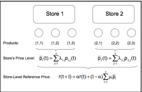
1.1 Formation of Reference Prices for a Duopoly Multiple-Product Setting . 16

2.1 Comparison of forecast accuracy of diﬀerent models . . . 23

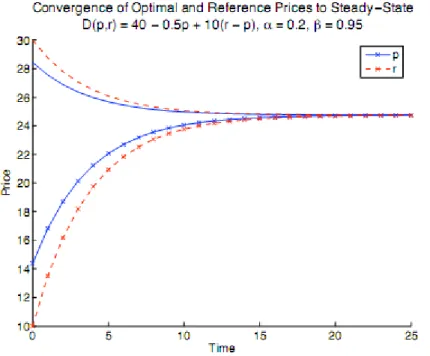
3.1 Optimal Price and Optimal Transition of Reference Price for a Monopoly 33

3.2 Convergence to Steady-State Reference Price for a Monopoly . . . 34

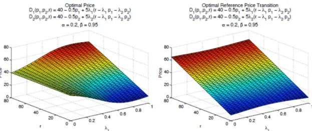
4.1 Optimal Pricing Policy and Reference Price Transition for the Two-Product case. . . 43

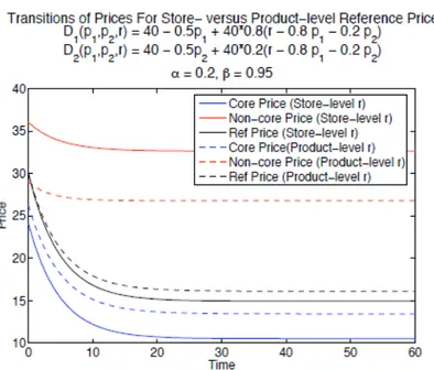
4.2 Transition of Prices and Reference Prices when Retailer Incorrectly As-sumes Individual Reference Price for Each Product . . . 44

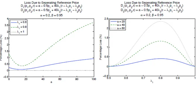
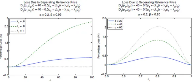
4.3 Eﬀects of Magnitude of Demand on Revenue Loss for Identical Products 45

4.4 Eﬀects of Price Sensitivity of Demand on Revenue Loss for Identical Products 46

4.5 Eﬀects of Magnitude of Reference Price Eﬀects on Revenue Loss for Iden-tical Products . . . 46

4.6 Eﬀects of Magnitude of Demand of the Core Products on Revenue Loss . 47

4.7 Eﬀects of Price Sensitivity of Demand of the Core Product on Revenue Loss 48

4.8 Transition of Prices and Reference Prices for Optimal versus Myopic Policies 49

4.9 Eﬀects of Magnitude of Demand on Revenue Loss of Myopic Policy for Identical Products . . . 50

4.10 Eﬀects of Price Sensitivity of Demand on Revenue Loss of Myopic Policy for Identical Products. . . 50

4.11 Eﬀects of Magnitude of Reference Price Eﬀects on Revenue Loss of Myopic Policy for Identical Products . . . 51

4.12 Eﬀects of Magnitude of Demand of the Core Products on Revenue Loss of Myopic Policy . . . 51

4.13 Loss of Revenue Due to Separating Reference Price and Myopic Policy with N Products . . . 53

5.1 Transition of Prices and Reference Prices when Retailers Ignore Competition 69

5.2 Eﬀects of Magnitude of Demand on Revenue Loss . . . 70

5.3 Eﬀects of Price Sensitivity of Demand on Revenue Loss . . . 70

5.4 Eﬀects of Magnitude of Reference Price Eﬀects on revenue Loss . . . 71

(14)

(15)

List of Tables

2.1 Demand and Probability Distributions . . . 17

2.2 Summary of U values for each forecasting method and history . . . 23

2.3 Occupancy and Price . . . 24

5.1 Discrepancy between Prices and Revenues of Heuristic and Equilibrium Policy . . . 68

(16)

Some Notations and Acronyms

Dj(p, r) The demand of product j as a function of the price vector p and the reference price r.

dj(pj) The demand of product j in absence of reference price eﬀect.

Rj(p, r) Product j’s reference price eﬀect.

g(p, r) The reference price dynamics. pi(t) Store i’s price level =

Pn

j=1 ipi,j(t), where n is the number of products.

p⇤ Optimal price.

p⇤⇤ _{The steady state of the sequence (p}⇤₎_.

r⇤ Optimal reference price.

r⇤⇤ _{The steady state of the sequence (r}⇤₎_.

Vector of nonnegative weights such that 10

= 1. ↵ Forecast smoothing coeﬃcient.

U Theil’s inequality coeﬃcient.

YM Yield Management. RM Revenue Management. MP Markov-Perfect Equilibrium. MAD Mean absolute deviation.

(17)

List of Tables 7

MPE Mean percent error.

MAPE Mean absolute percent error. MSE Mean square error.

(18)

(19)

Chapter 1

Introduction

1.1 Motivations and Overview

Revenue management (RM), also known as yield management, is described as providing the right product, at the right time, to the right customer, for the right price (Smith et al. [40]). RM has been used extensively in the airline, hotel, and car rental industries. Firms use RM strategies, such as pricing and capacity allocation to maximize revenues while delivering the same service to customers.

In the airline industry, airlines seek to maximize their revenue by using booking policies to price seats. When a customer requests a seat in a booking class at a certain fare, the airline must decide whether to accept or reject this request. Generally, this decision is complex since there are numerous factors which aﬀect the revenue gained from this customer (McGill and van Ryzin [34]).

In the hotel industry, hotels can increase their revenue by matching demand to the rooms available using forecasts from historical data. Similarly to airlines, hotels ultimately must decide whether to accept or decline a booking request, depending on the customer’s length of stay, arrival rate, and room rate (Vinod [43], Weatherford and Kimes [45]). The capacity allocation methods used in RM subscribe mainly to two approaches:

• An allocation performed based on a probabilistic demand forecasting or EMSR method (Expected Marginal Seat Revenue), with a calculation of the expected revenue by fare class.

(20)

10 Chapter 1. Introduction

• An Allocation by price floors or Bid Prices determining the acceptance or rejection of the proposed reservation at a certain price. This method is commonly used for the optimization of complex networks.

The two approaches, EMSR and Bid Price, can also be combined (For more details about these methods refer to Talluri and Van Ryzin [42]).

The eﬀectiveness of these methods depend on the quality of demand forecasts. In the hotel industry, the room demand forecasting phase, considered as a pre-processing step in revenue management, should be studied in detail since it determines the reliability of the optimization part. The accuracy of the forecast can lead to the extreme situations of potentially sizable profits or completely inaccurate room allocations. Weatherford and Kimes [48] show that exponential smoothing, pickup, and moving average models are the most robust.

Traditional literature in pricing and inventory allocation assumes that there is no interaction between the firms and their customers. While this assumption is often crucial to the analysis of the models, it can be very unrealistic. As a result, more sophisticated pricing models that incorporate customer behavior have emerged in recent years.

A branch of the dynamic pricing literature has taken a particular interest in the concept of a reference price. For businesses that have a repeated interaction with customers, expectation of price is formed through past experience. Subsequently, the utility of consumption is aﬀected when there is a mismatch between the current and the expected price. For example, if an ice cream shop that used to charge $4 for a classic cone increases the price to $5, it will immediately have a negative impact on the frequent customers and hence the demand. Over time, however, customers will adjust their expectation and the demand may be restored to the previous level.

We extend the concept of reference price to multi-product pricing by introducing the notion of store’s price level. The idea is motivated by a survey article of McKinsey & Company on price promotions in Latin America (Calicchio and Krell [10]). The authors find that a surprisingly small number of products (less than 4 on average) account for half of the information customers use to determine their perceptions of a store’s price level. These products are usually the generic, most commonly used household items, such as sugar, cooking oil, and detergents etc. We will refer to these as the "core" products.

The realization of this eﬀect has important pricing implications. For instance, if the retailer can identify what his core products are, then he can benefit from pricing these products competitively. While the retailer is foregoing some of the revenue from these products, he is improving the customers’ perception of his store’s price level, thereby attracting more customers to shop at the store. Consequently, the retailer

(21)

1.2. Literature Review 11 can benefit from the increases in sales of other, perhaps higher margin products. To illustrate this point, let us consider a gas station. The price of gasoline is the most important determinant of a consumer’s choice of urban gas stations. At the same time, although the price of gasoline has been increasing over the past five years, the profit margin of consumer’s gasoline remains thin. In 2004, the national average of gasoline mark-up was 12.7 cents per gallon, and this average does not increase with price itself (Kelly [24]). Therefore, it can be extremely beneficial for gas stations to set the price of gasoline competitively to lure price-sensitive customers, and reap the ben-efit of an increase in sales of in-store products, as these products enjoy a 20-30% mark-up. The concept of reference price (both at product and store level) also provides a good framework for modeling competition. The economics literature models competition in the market by directly assuming that the demand of a product is a function of its com-petitor’s price, in addition to its own price. We propose an alternative model where the retailers compete through their influences on the reference price for the single-product case, and through the customers’ perception of the stores’ price level for the multi-product case. Our discrete-time formulation yields closed-form solutions for optimal pricing poli-cies that are functions of state variables that represent the market environment, namely the reference prices. This approach lends itself well to managers as the results can be practically implemented, in contrast to the continuous-time approach whose solutions are expressed as functions of time, which are less useful in practice.

1.2 Literature Review

In recent years, the topic of dynamic pricing with consideration of customer behavior has attracted a lot of attention in both academic research and industry practice. Elmaghraby and Keskinocak [12] noted that this is an important element that, in the past, was largely missing from the academic literature and price optimization software.

To incorporate the effect of customer’s behavior into pricing, a number of papers have investigated the impact of past prices on the customer’s utility of the current consumption. Earlier papers in this area focus mainly on how customers form a reference price of a product from their past experiences, and how the reference price affects the demand. More recently, the interest has shifted towards finding optimal pricing strategies with reference price effects.

The most common framework for the formation of the reference price is an exponentially weighted average of the past-observed prices, where consumers are given memory parameters associated with past prices (see Winer ([50], [51]), Kalwani et al. [23], Krishnamurthi et al. [27], Putler [38], and Greenleaf [16] for more details). However,

(22)

12 Chapter 1. Introduction several other approaches exist as well. Hardie et al. [18] argue that customers do not form a reference price from the past-observed prices due to the lack of memory; instead the price of the most recent purchase alone is the reference price. Some methods for reference price formation include other information such as market share (Winer [51]), price trends, deals proneness of customers, frequencies of promotions, and store characteristics (Kalwani et al. [23]). To compare the effectiveness of the different reference price models, Briesch et al. [7] put each model to test against scanner panel data. The effectiveness of the models are measured on the basis of fits and predictions, and efficiencies if the results are close. Overall, they find the weighted average of past prices to be the most effective.

It is generally accepted in the literature that the impact of reference price on demand is a function of the diﬀerence between the current price and the reference price. Customers perceive a gain when the price is below the reference price, and a loss if it is above. The seminal work of Kahneman and Tversky [22] on Prospect Theory predicts that there is an asymmetry in customers’ perception of gains and losses. Specifically, customers’ perception of loss is greater than that of gain for the same magnitude of price diﬀerentials. Customers with such perceptions are said to be "loss averse". Winer [50] proposes that the impact on demand should also be asymmetric in a similar fashion. Many empirical studies have been performed to validate this proposal. Putler [38] tests this theory with data from eggs sales and Hardie et al. [18] use data from orange juice to test the multinomial logit framework of reference brand. However, Greenleaf [16] finds that there may be times when the impact of gain is greater than that of loss. In contrast, these customers are said to be "loss seeking". In the context of multiple brands, Krishnamurthi et al. [27] provide empirical evidence that shows that the impact of loss on demand is less than or equal to gain for brand switchers and vice-versa for brand-loyal customers.

For most of the literature in dynamic pricing under reference price effects (e.g., Kopalle et al. [25], Greenleaf [16], Kopalle and Winer [26], Popescu and Wu [37]), one common difficulty is deriving explicit solutions of a non-smooth optimization problem for the optimal policies. Consequently, the results are usually obtained through numerical procedures (e.g., dynamic programming and Monte-Carlo simulation). To tackle this problem, Fibich et al. [14] formulate the problem in continuous-time and present a two-stage method to obtain explicit solutions for optimal prices. They claim that their result is the first explicit expression of an optimal pricing policy for symmetric reference price effect, and contribute their success to the advantage of continuous-time over discrete-time formulation. "The discrete formulation is convenient for numerical simulations... but cumbersome for obtaining explicit solutions". While their solution in continuous-time provides an elegant proof of monotonicity and convergence, we believe that a solution in discrete-time is more valuable to managers, since it is more realistic

(23)

1.3. Contributions 13 and easier to implement in practice. In this thesis, we present such a solution. Also, Arslan et al. [2] extend the concept of reference price and the method by Fibich et al. [14] to study competition in innovation and pricing for industries with short-life products. Arslan et al. [3] use a reference price model to solve the optimal timing of the introduction of new products and their pricing.

Another popular and relevant field of pricing is that of pricing in the presence of strate-gic customers. In contrast to the customer behavior considered in the reference price literature, strategic customers use their anticipation of future prices to aid their decision, rather than their experience of the past prices. Examples of work in this area include Gallego et al. [15], Liu and van Ryzin [31], Milner and Ovchinnikov [35], Levin et al. [29], Anderson et al. [1], and Asvanunt and Kachani [4].

1.3 Contributions

In this thesis, we make the following contributions:

• We discuss various forecasting models used in hotel revenue management. We focus on the measurement of model accuracy, which is critical to selecting the forecasting method that provides the best stochastic demand distribution for the optimization phase. We report on computational results based on real-life data.

• We derive a closed-form solution of the optimal pricing policy for a monopolist selling a single product, under linear demand and reference price-eﬀect assumptions. Fibich et al. [14] solved the problem for a single product in continuous-time. Our approach yields the optimal policy in discrete-time as a function of the state, that is the current level of the reference price, and is much more practical than the continuous-time solution, which was provided as a function of time.

• We extend the previous result and derive a closed-form solution of the optimal pricing policy for a monopolist selling multiple products, when the reference price eﬀect is at the store’s level, and show that the monotonicity and convergence results still hold. We provide numerical analyses for the case of two products. We find that for otherwise identical products, the steady-state price of a core product is lower than that of a non-core product. We compute the retailer’s loss of revenue if he incorrectly assumes the reference price eﬀect to be at the product level and prices the products individually.

• We develop a reference price model for competition in a duopoly market for a single product. We derive a system of equations that we solve numerically to derive Markov-Perfect (MP) equilibrium pricing policies. We provide a closed-form heuristic and demonstrate numerically that it is very close to the equilibrium.

(24)

14 Chapter 1. Introduction

• We derive closed-form solutions for pricing policies of a retailer who is an optimizer when his competitor follows one of three diﬀerent suboptimal policies, and prove monotone convergence of these solutions to their respective steady states. We per-form numerical analyses to study the impact on revenue when both retailers ignore competition. We find that pricing at the equilibrium generally yields lower rev-enue than pricing when both retailers ignore competition, unless one retailer has very little influence on the market. Finally, we illustrate how our approach can be extended for duopolists with multiple products, and how a similar closed-form heuristic may be obtained.

1.4 General Pricing Model and Formulation

We begin by considering the optimal dynamic pricing policy for a monopolist oﬀering one product. Then, we extend our model to the multi-products case. The monopolist wishes to maximize his revenue over an infinite time horizon. The store faces deterministic homogenous customer arrival over time. We formulate the optimization problem in discrete time.

At each time period, the demand for product j, Dj(p, r), is a function of the price vector,

p, and the reference price of the store, r. Furthermore, Dj(p, r) can be separated into

two additive components. First is demand in absence of reference price eﬀect, denoted by dj(pj), and second is the reference price eﬀect, denoted by Rj(p, r). Thus,

Dj(p, r) = dj(pj) + Rj(p, r), f or j = 1, ..., N

Throughout this thesis, we assume that both components of the demand are linear. Specifically, we assume the following:

dj(pj) = aj bjpj

Rj(r, p) = c j(r

0

p)

where aj, bj, and c are positive and is a vector of nonnegative weights such that

10 = 1. In other words, 0p is the weighted average price of the firm’s products, and is interpreted as the current store’s price level.

By modeling the magnitude of the reference price eﬀect as c j(r

0

p), we assume that the eﬀect on each product is proportional to the product’s influence on the reference price itself. Alternatively, we can view the reference price eﬀect to be at the store level. Namely, the overall increase on demand of the entire store is c(r 0

p), and is allocated to each product proportionally according to . The weight j is interpreted

(25)

1.4. General Pricing Model and Formulation 15 store’s price level represents the expensiveness of the store, the correct formula should be c j(r

0

(p q)), where q is a vector used to normalize prices such that pj qj measures

the expensiveness of product j. For the sake of simplicity, we omit q from the analy-sis by assuming that all products have the same intrinsic values without loss of generality. Furthermore, we assume that customers are loss neutral, i.e. the reference price eﬀect is symmetric for both loss and gain. Our results extends to asymmetric reference price eﬀects using the same methodology as in Popescu and Wu [37].

We assume that the reference price evolves over time according to the customers’ expe-rience and exposure to the price information. In other words, the reference price at the next time period is a function of the current reference price and the current store’s price level, 0

p. Specifically, we model the evolution of the reference price as follows r(t + 1) = g(p(t), r(t)) = ↵r(t) + (1 ↵) 0p(t),

where 0  ↵ < 1. Thus, the optimal dynamic pricing policy for the retailer is the solution to the following optimization problem:

max 1 X t=0 t_{D(p(t), r(t))}0 p(t) s.t. r(t + 1) = g(p(t), r(t))_8t 0, where 0 < < 1 is the discount factor.

Further ahead in this thesis, we consider retailers in a duopoly market, each selling multiple products. Similar to the monopoly case, the demand for product j from retailer i is given by

Di,j(pi, r) = di,j(pj) + Rj(pi, r), f or i = 1, 2 and j = 1, ..., N,

where

di,j(pi,j) = ai,j bi,jpi,j

Ri,j(r, pi) = ci i,j(r

0

ipi)

In this case, the reference price is the customers’ perception of the market value of the stores’ price levels. We introduce a vector µ, which corresponds to the store’s influence on the customer’s perception of the reference price. In other words, the customers take the store’s price levels, 0

ipi, for each retailer i, and form a current market store’s price

level as Piµi

0

(26)

16 Chapter 1. Introduction The reference price at the next time period is a function of the current reference price and the current market store’s price level. Specifically, the reference price evolves according to: r(t + 1) = g(p1(t), p2(t), r(t)) = ↵r(t) + (1 ↵)(µ1 0 11p1(t) + µ2 0 2p2(t))

In this setting, each retailer chooses a pricing policy that maximizes the present value of its revenue over infinite horizon, as in the monopoly case above.

Figure 1.1 illustrates the interaction between the products from each store in the forma-tion of the reference price.

(27)

Chapter 2

Forecasting and Decision Making

2.1 Demand Behavior

In the airline industry, the observed data on passenger demand, passenger cancellations, passengers showing at boarding, no-show passengers, and go-show passengers are gener-ally estimated by standard probability laws. [13]

Data Estimation Authors Airline

Demand Normal Distribution Buhr [9] Lufthansa

Normal Distribution [17] Lufthansa

Normal Distribution Belobaba [5] Western Airlines Poisson Distribution Rothstein [32] American Airlines Poisson Distribution Buhr [9] Lufthansa Poisson Distribution Alstrup [19] SAS

Poisson Distribution Lee [36] SAS

Poisson Distribution Weatherford [44] SAS Binomial Distribution Brumelle [8] SAS Binomial Distribution approximated by

Normal Distribution Schlifer and Vardi [39] El Al Airlines Cancellations Binomial Distribution Rothstein [32] American Airlines

Binomial Distribution approximated by

Normal Distribution Alstrup [19] SAS

Passengers at the Boarding Normal Distribution Schlifer and Vardi [39] El Al Airlines No-Show Binomial Distribution approximated by

Normal Distribution Alstrup [19] SAS

Go-Show Binomial Distribution Rothstein [32] American Airlines Table 2.1 – Demand and Probability Distributions

(28)

18 Chapter 2. Forecasting and Decision Making Analyses of the behavior of passengers demand have given rise to some simplifying assumptions, notably the Forgetfulness Law and Early Bird.

Forgetfulness law:

Using a statistical study on data from the Spanish Airline Iberia, Martinez and Sanchez [33] showed that :

• For international reservations on long-haul flights, the cancellation probability was independent of the booking date.

• For reservations on domestic flights, there is a negative linear relationship between the booking date and the probability of cancellation. The cancellation is less likely to happen in the case of a close-to-departure booking.

These results are valid for individual reservations as well as for group reservations. In fact, it is diﬃcult to generalize these "laws" to all airlines whose structures and networks can be very diﬀerent. Moreover, the air transportation business has undergone radical change over the last 40 years. However, the Forgetfulness Law is an underlying assumption to most optimization models for convenience.

Early Bird:

Littlewood [20] introduced the Early Bird assumption stating that low-contribution pas-sengers make reservations before high-contribution paspas-sengers. Even though this assump-tion does not truly represents the behavior of passengers on the entire reservaassump-tion period (Lee et al. [28]), it has the advantage of avoiding dynamic approaches and thus consider-ably simplifying the calculations. In addition, it doesn’t seem to aﬀect the performance of models that use it.

2.2 Demand Forecasting Models in the Airline and

Ho-tel Industries

The goal of forecasting in the airline/hotel industry is to provide an estimated customer demand for seats/rooms as well as an estimate of a number of behaviors, such as cancellations or no-shows, in order to make the most of the optimization techniques. It is a crucial step to setting bookings limits for a particular class of customers (i.e. accepting or rejecting an airline/hotel reservation).

Demand forecasting methods in revenue management fall into one of three main categories (Zakhary et al. [53]):

(29)

2.2. Demand Forecasting Models in the Airline and Hotel Industries 19

• Historical booking models forecast the final demand by considering only the recorded past data, of the final number of rooms or arrivals on previous nights, to predict customers behavior in time series.

• Advanced booking models include only the observed buildup of reservations over time for a particular stay night, which Lee et al. [28] call the "development of the booking curve". These models estimate the rate of increased reservation (pick up) in each booking period and then aggregate all future increased reservation to obtain the final forecast of the booking curve.

• Combined models integrate historical and advanced booking models via either re-gression or weighted average methods (Weatherford and Kimes [48]).

In what follows, we present forecasting models that are used the most. Weatherford and Kimes [48] provide a detailed discussion about various forecasting methods. Based on a statistical study of passenger demand, they indicate the models that give the best results: moving averages, exponential smoothing, linear and logarithmic regressions, and the Pickup model.

• Moving Averages: Consider the simple case of a demand on a flight for diﬀerent days of the week. A naive forecast is to assume that the demand observed on day t happens again the next day, ie:

Ft+1= Dt

or use the simple moving average on a few days (4 days is often used), namely, Ft+1 =

Dt+ Dt 1+ Dt 2+ Dt 3

4

• Exponential Smoothing: Simple exponential smoothing is similar to moving averages, but the forecasts are revised according to the most recent experience:

Ft= ↵Dt 1+ (1 ↵)Ft 1

where ↵ is a smoothing constant between 0 and 1.

The closer ↵ is to 0, the stronger is the memory of the phenomenon and the less reactive is the forecast. The closer ↵ is to 1, the greater is the weight of the present and the greater is the prediction sensitivity to change.

In practice, ↵ is chosen in a way to minimize the mean absolute percent error (MAPE) applied to the data.

(30)

20 Chapter 2. Forecasting and Decision Making

• Pickup Method: Consists in adding to the current bookings the average bookings to come till departure estimated from the history. The main idea of using the pickup method is to estimate the increments of bookings (to come) and then aggregate these increments to obtain a forecast of total demand to come (Talluri and Van Ryzin [42]). Pickup is defined as the number of reservations picked up from a given point of time to a diﬀerent point of time over the booking process (Weatherford and Kimes [48]), which identifies the estimated increase of booking in each period and then accumulate all data into a total demand that is arriving in the future. (Zakhary et.al [53])

– Classical PickupIn the classical pickup method, only the booking data for completed booking curves are used in the forecasting process (Talluri and Van Ryzin [42]). The Classical pickup method hence ignores available information of incomplete arrival dates that might be useful (Zeni [54]).

– Advanced PickupThe Advanced pickup method, on the other hand, uses all the available complete and incomplete booking data (Talluri and Van Ryzin [42]) in the forecasting phase. Hence, it uses reservation data of arrival dates that still did not occur to make better forecasts, instead of relying only on complete arrival histories.

For more details and illustrations of the Pickup Method and its variations (Additive vs Multiplicative, Classical vs Advanced, Simple Average vs Weighted Average) refer to Zakhary et al. [53].

Forecasting applied to Hotel/Airline Revenue Management should take two time-related variables: the time of booking (i.e. reservation date) and the time to consumption (i.e. number of days out) (See Weatherford and Kimes [48] for more details). We will look at the diﬀerent forecasting methods existing in terms of data treatment (e.g. historical vs. actual) and eﬃciency. In addition to the choice of the best forecasting method, other very important issues, such as the forecast base, the levels of aggregation, the forecast period, the selection of data, the treatment of outliers and the measurement of the forecast’s accuracy should be considered.

Weatherford and Kimes [47] show that fully disaggregated forecasts generally produce better results than partial or fully aggregated approaches, which means that hotels should track arrival by length of stay and rate category.

One important issue to consider is how to divide time to provide a good basis for a forecast. It is common practice to take a week as a forecast, and therefore consider each day diﬀerently. For instance, forecasts for Mondays only depend on other Mondays’ data, and so on. Another point to address is the seasonality phenomenon, which is particularly important for the hotel business. Considering a small dataset may prevent managers from capturing seasonality. On the other hand, using too many periods (i.e.

(31)

2.3. Forecast Accuracy 21 considering very old data) may make the forecast unresponsive and not dynamic enough. Because prior research has looked at forecast accuracy (Weatherford and Kimes, [48]), we focus on using partial versus full history. Using real hotel data, we test our model with four, eight, and twelve weeks of data history.

In our study, we use the following forecasting methods: • Classical Pickup (Duncanson, [11])

• Advanced Pickup (L’Heureux, [30]) • Linear Regression (Wickham, [49])

• Simple Exponential Smoothing with ↵ = 0.15 (Wickham, [49]) • Simple Exponential Smoothing with ↵ = 0.35 (Wickham, [49])

• Advanced Pickup + Exponential Smoothing with ↵ = 0.15 (Wickham, [49]) • Advanced Pickup + Exponential Smoothing with ↵ = 0.35 (Wickham, [49])

2.3 Forecast Accuracy

Lee [36] shows that for the airline business, a 10% improvement in accuracy may contribute up to 3% increase in revenue, which would impact the net income in a much larger way due to the small margins existing in the airline industry. Accuracy is perhaps the most important issue in forecasting since it directly determines the choice of a method.

The room demand forecasting phase, considered as a pre-processing step in hotel revenue management, should be studied in detail since it determines the reliability of the optimization phase. The accuracy of the forecast can lead to the extreme situations of potentially sizable profits or completely inaccurate room allocations.

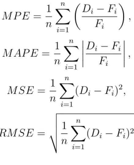
Several measures of the forecast performance exist. The Mean Absolute Deviation (MAD) is the simplest and most widely used. It consists in averaging the absolute values of the forecast errors. The Mean Percent Error (MPE) is defined as the average of percentage errors. The Mean Absolute Percent Error (MAPE) is similar to the MPE except that it averages the absolute values of the forecast errors. The Mean Square Error (MSE) considers the mean of the squared forecast errors. The Root Mean Square Error (RMSE) is the square root of the MSE.

M AD = 1 n n X i=1 |Di Fi|,

(32)

22 Chapter 2. Forecasting and Decision Making M P E = 1 n n X i=1 ✓ Di Fi Fi ◆ , M AP E = 1 n n X i=1 Di Fi Fi , M SE = 1 n n X i=1 (Di Fi)2, RM SE = v u u t 1 n n X i=1 (Di Fi)2

Of the mentioned measurements, MPE and MAPE seem the more relevant since they produce dimensionless numbers. However they remain undefined when the total final number of booking is zero, which is possible (Wickham, [49]).

To overcome this drawback, we use a measure called Theil’s Inequality Coeﬃcient, de-noted by U (Scandinavian Airlines System, 1974), defined as follows:

U2 =

X ( ˆF F )2

n X F2

n

where ˆF and F are the actual and forecasted final room bookings from n observations. The numerator, equal to MSE, allows to determine the forecast error, while the denom-inator, equal to the mean square forecast, normalizes the indicator. This coeﬃcient presents the double advantage to be dimensionless and always defined which makes it a very good indicator to determine the relative performance of the various methods described before.

For an errorless forecast, U is equal to 0. For all forecasting models, the further away its U value is from zero, the worse the forecast (Wickam, [49]).

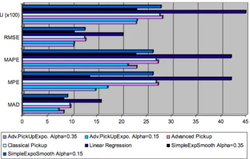
Figure 2.1 presents the diﬀerent measures of forecast accuracy for the methods used here. It shows that Linear Regression is by far the poorest method in term of forecast accuracy and that the combined models perform well whatever the indicator employed. However, the diﬀerences are very small among all the combined methods considered, so the model should be chosen on a case by case basis.

The measurement of model accuracy is critical to selecting the forecasting method that provides the best stochastic demand distribution for the optimization phase.

(33)

2.3. Forecast Accuracy 23

Figure 2.1 – Comparison of forecast accuracy of diﬀerent models

Forecasting Method 4 weeks 8 weeks 12 weeks Classical Pickup 7.1813 6.9322 6.7699 Advanced Pickup 7.1813 6.9322 6.8059 Linear Regression 6.2852 7.3284 6.9940 Simple Exponential Smoothing

with ↵ = 0.15 6.6380 5.8685 5.8944 Simple Exponential Smoothing

with ↵ = 0.35 6.2495 5.9880 6.0523 Advanced Pickup + Exponential

Smoothing with ↵ = 0.15 6.2629 6.0776 5.9439 Advanced Pickup + Exponential

Smoothing with ↵ = 0.35 6.3828 6.2209 6.1276 Table 2.2 – Summary of U values for each forecasting method and history

(34)

2.4 Yield Management

Occupancy and price: Two key factors in determining total revenue. This is the heart of Yield Management(YM).

We illustrate that by the following example where three airlines are selling 400 seats in planes featuring two airfare classes. The table below summarizes the result:

Airline A Airline B Airline C Number of Seats Sold at $500 80 248 192 Number of Seats Sold at $350 280 40 132 Total Number of Seats Sold 360 288 324 Occupancy Rate 90% 72% 81%

Unit Revenue $383.3 $479.2 $438.9 Total Revenue $138K $138K $142K

Table 2.3 – Occupancy and Price

• Airline A achieves the best occupancy rate.

• Airline B achieves the best average price per passenger.

• Airline C practices Yield Management: It looks for –based on the demand forecast– the best balance between occupancy and price to maximize its total revenue. Airlines should aim to maximize their financial occupancy rate, that is the ratio of the realized and the potential flight earnings, and thus exceed the concept of physical occupancy coeﬃcient.

Yield Management is a form of price discrimination. It aims to maximize the income of the company under the constraint of an available capacity that must be allocated according to the expressed demand. For this, the company must manage both the inventory (or perishable stock of available units) and pricing, that is adapting the oﬀer to the demand by the system of pricing. According to the most famous definition, it is a method allowing a firm to sell the fair share of the available capacity to the right customer at the right time and the right price.

Four conditions are necessary for the application of Yield Management:

• A perishable inventory and/or a seasonal demand that makes the time of selling important.

(35)

2.4. Yield Management 25

• High fixed costs and relatively low marginal costs of selling an additional unit. • A fixed capacity either in whole or in short-term.

• The possibility of buying or booking the products or services in advance.

These conditions apply to most services providers, which explains the rapid spread of Yield Management. With its beginning in the airline industry, YM is used today in:

• Hotels, Resorts, and Amusement Parks (Marriot, Holiday Inn, Hilton, Accor, Club Méditeranée, Disney Land...)

• Cruise Lines (Royal Caribbean, Carnival, Disney...)

• Passenger Rail Transport and Sea & Rail Freight Transport (Amtrack, SNCF, SeaLand, Eurotunnel...)

• Car Rentals (Avis, Hertz, National, Europcar...)

• Theatrical Business (Disney Theatrical Productions with "The Lion King" becom-ing the top-grossbecom-ing show on Broadway in 2013, an unprecedented feat for long-running musicals)

• Media (CBC, ABC, TF1,...) And more...

Capacity allocation, also known as inventory control in the airline business, consists in the search of optimality in the capacity (seats) supply management. It encompasses the set of all decisions of allocating capacity to the diﬀerent booking classes.

The methods used in RM subscribe mainly to two approaches:

• An allocation performed based on a probabilistic demand forecasting or EMSR method (Expected Marginal Seat Revenue), with a calculation of the expected revenue by fare class.

• An Allocation by price floors or Bid Prices determining the acceptance or rejection of the proposed reservation at a certain price. This method is commonly used for the optimization of complex networks.

The two approaches, EMSR and Bid Price, can also be combined. The discussion of these methods and their variants is beyond the scope of this thesis. For more details about these methods refer to Talluri and Van Ryzin [42].

The eﬀectiveness of these methods depend on the quality of demand forecasts. Indeed, capacity allocation management depends on the quality of the forecast, but the previous capacity allocation policy has already produced eﬀects on the demand currently observed. In fact, several demand reactions to a capacity constraint must be taken into account:

(36)

• An additional demand due to diversion (booking in a higher class because of un-availability in the desired class)

• An additional demand in a fare class due to the closing of an equivalent class in another flight

• A loss of a potential demand as a result of a class closure

Booking curves must represent the potential demand, that is the demand in case of providing 100% capacity, called the unconstrained demand. Detruncation should be handled with caution to avoid both the spill (loss of earnings on the most profitable customers) and the spoilage (refusal of a low-contribution passenger/wasted capacity) if it is too large.

Belobaba [6] proposes a method to reconstruct the unobserved demand as a result of closure.

(37)

Chapter 3

Dynamic Pricing Model with a

Reference Price Eﬀect in a Monopoly

Market

Based on: S. Kachani, Y. Oumanar and N. Raissi, A Closed-Form Solution for a Dynamic Pricing Model with Reference Price Eﬀect, App. Math. Sc.

Abstract: This chapter addresses the problem of pricing for an airline or a retailer selling one product to a stream of repeated customers over an infinite time horizon. We propose a dynamic pricing model that incorporates the concept of customers’ reference price. We derive an optimal pricing policy and prove its monotone convergence in a monopoly context. We derive an analytical result for the optimal prices. Our pricing policy is a function of the current market condition, represented by the reference price, as opposed to the previous studies where the pricing policy is a function of time.

Keywords: Dynamic Pricing, Reference Price, Management Decision making, Dynamic Optimization

3.1 Introduction

Dynamic pricing, also known as time-based pricing, is a strategy that adjusts the product price in real-time in order to maximize the profit. Dynamic pricing is particularly suitable for the travel industries, such as airlines, because inventory cannot be replenished and unsold products have little salvage value. An airline has incentive to dynamically adapt its pricing to the demand. Interested readers can refer to Elmaghraby and Keskinocak [12], McGill and Van Ryzin [34], or Weatherford and Bodily [46] for a general survey on dynamic pricing and its role in revenue management.

Traditional literature in airline pricing assumes that there is no interaction between the firms and their customers. However, customers have a memory of past ticket prices and they develop a kind of price expectations. These price expectations are called reference prices. They become benchmark prices against which customers compare the current tickets prices before they make purchases. If the reference price is below the observed price, customers perceive gains and purchasing becomes more attractive (Hardie et al. [18]). For a review of the theoretical foundations and modeling of the reference price concept we refer the reader to Winer [52].

This chapter presents a dynamic pricing model in the airline industry incorporating the concept of customer’s reference price.

3.2 Dynamic Pricing Formulation

We are making the assumption that the airline is only selling one class category at a time and we will consider the demand function as being generated by:

D(p, r) = a bp + c(r p) as in Kopalle [25] and Fibich et al. [14].

The reference price is following the dynamic:

r(t + 1) := g(p(t), r(t)) = ↵r(t) + (1 ↵)p(t) The airline decision problem takes the following form:

Find: V⇤(r0) = sup (p0,p1,...) 1 X t=0 t_{D(p(t), r(t))p(t)} s.t. r(t + 1) = g(p(t), r(t))

(39)

3.2. Dynamic Pricing Formulation 29 We can write the simplified Bellman equation dropping the time subscript:

V⇤(r) = sup

p D(p, r)p + V

⇤_{(g(p, r))} _(3.1)

The optimal value function that solves the Bellman equation (3.1) is given by: V⇤(r) = r2 + r + " (3.2) which is attained by the following pricing policy

p⇤(r) = a + (1 ↵) + r(c + 2 ↵(1 ↵) 2(b + c (1 ↵)2₎ (3.3) where = b(1 ↵ 2 _{) + c(1} _{↵ )} p_(b(1 _↵2 _{) + c(1} _{↵ ))}2 _c2₍₁ _↵)2 2(1 ↵)2 (3.4) = a(c + 2(1 ↵)↵ ) 2b(1 ↵ ) + c(2 ↵ ) 2(1 ↵)2 (3.5) " = (a + (1 ↵) ) 2 4(1 )(b + c (1 ↵)2 ₎ (3.6) Theorem 1.

In order to solve equation (3.1) we state the postulate that the optimal value function is quadratic and given by:

V⇤(r) = r2 + r + " where , and " are to be found.

Hence, (3.1) becomes: V⇤(r) = sup

p (a bp + c(r p))p + ((↵r + (1 ↵)p)

2 _{+ (↵r + (1} _{↵)p) + ")} _(3.7)

The optimal price p⇤_(r) _{results from writing the partial derivative of V (r) with respect}

to p and setting it equal to 0. Solving @V (r)

@p = 0 for p yields the optimal pricing policy

p⇤(r) = a + (1 ↵) + r(c + 2 ↵(1 ↵) 2(b + c (1 ↵)2₎

By plugging (3.3) into (3.7) and then collecting the coeﬃcients of the polynomial we determine , and ":

(40)

30 Chapter 3. Dynamic Pricing Model with a Reference Price Eﬀect in aMonopoly Market " = (a + (1 ↵) ) 2 4(b + c (1 ↵)2 ₎ 1 1 , = a c + 2↵(1 ↵) 2(b + c (1 ↵)2 ₎+ (1 ↵)(c + 2↵(1 ↵) ) 2(b + c (1 ↵)2 ₎ + (a + (1 ↵) )(c + 2 ↵ (1 ↵)) 2(b + c (1 ↵)2 ₎ 2(b + c (1 ↵)2_{)(a + (1} _↵) _{)(c + 2↵(1} _↵) ₎ 4(b + c (1 ↵)2 ₎2 + ↵ = (a + (1 ↵) )(c + 2↵(1 ↵) ) 2(b + c (1 ↵)2 ₎ 1 1 ↵ = a(c + 2↵(1 ↵) ) 2(b + c (1 ↵)2 ₎₍₁ _{↵ )} ₍₁ _{↵)(c + 2↵(1} _↵) ₎ = a(c + 2↵(1 ↵) ) 2b(1 ↵ ) + c(2 ↵ ) 2(1 ↵)2 , = (c + 2↵(1 ↵) )(c + 2 ↵ (1 ↵)) 2(b + c (1 ↵)2 ₎ + ( b c + (1 ↵)2_{)(c + 2↵(1} _↵) ₎2 (4(b + c (1 ↵)2 ₎2 + ↵ 2 = (c + 2↵(1 ↵) ) 2 4(b + c (1 ↵)2 ₎ 1 1 ↵2

Hence, is the smaller root of the quadratic equation:

(1 ↵)2 2 (b(1 ↵2 ) + c(1 ↵ )) + c2/4 = 0 (3.8) Therefore,

= b(1 ↵

2 _{) + c(1} _↵ p_(b91 _↵2 _{) + c(1} _{↵ ))}2 _c2₍₁ _↵)2

2(1 ↵)2

Later, we will show that this choice of guarantees that is positive.

Since the value function V⇤_(r) _{represents the present value of the total revenue, it must}

be positive and increasing in r for all values of r 0. Given the uniqueness of V⇤_(r)

(Stockey et al. [41], it suﬃces to show that the coeﬃcients , and " are nonnegative real numbers in order to establish that our postulate is valid.

First, we will establish that is positive. Recall that is a solution of the quadratic equation (3.8). Suppose that the quadratic equation has real roots, then it is easy to see that both roots are positive since the coeﬃcients of the quadratic and the constant terms are positive, whereas the coeﬃcient of the linear term is negative.

To show that the roots are real, we only need to show that the term inside the square-root in (3.4) is always nonnegative. this is true because:

(41)

3.2. Dynamic Pricing Formulation 31 Next, to show that is well defined and positive, we need to show that

< 2b(1 ↵ ) + c(2 ↵ ) 2(1 ↵)2

This is true if and only if

b(1 ↵2 ) + c(1 ↵ ) p(b(1 ↵2 _{) + c(1} _{↵ ))}2 _c2₍₁ _↵)2

 2b(1 ↵ ) + c(2 ↵ )

, b((1 (1 ↵)2) 1) + c( 1) <p(b(1 ↵2 _{) + c(1} _{↵ ))}2 _c2₍₁ _↵)2

which holds because the left hand side is negative. Finally, " is well-defined and positive if and only if

< b + c

(1 ↵)2 (3.9)

which is again true because b and c are positive and b(1 ↵2 _{) + c(1} _{↵ )}_{ 2(b + c).}

Now that we established the validity of the postulate, the correctness of p⇤_(r)_{, and proved}

the result of the Theorem, we can derive the expression for the transition of the reference price under the optimal pricing policy, g⇤_{(r) = g(p}⇤_{(r), r)}_{. It is given by:}

g⇤(r) = (2↵(b + c) + c(1 ↵))r + (1 ↵)(a + (1 ↵) )

2(b + c (1 ↵)2 (3.10)

Finally, the steady state reference price r⇤⇤ _{is determined by solving r}⇤⇤_{= g}⇤_(r⇤⇤₎_.

r⇤⇤ = a + (1 ↵) 2b + c 2(1 ↵) = a(1 ↵ )

c(1 ) + 2b(1 ↵ ) (3.11) The second equality is not straight forward and follows from tedious calculations that involve substituting the expression for as given in (3.5), and using (3.8) to complete the square in the denominator.

The expression of r⇤⇤_{in (3.11) is the same equation (13) of Fibich et al. [}₁₄_{]. Because of}

the dynamic of the reference price, it is easy to see that the optimal price at the steady state must be the same as the reference price, i.e. p⇤⇤_{:= p}⇤_(r⇤⇤_{) = r}⇤⇤_.

(42)

3.3 Monotonicity and Convergence Results

Let’s first define the sequences of optimal reference prices (r⇤₎_{and optimal prices (p}⇤₎_as

follow:

r⇤(t) = g⇤(r⇤(t 1)) p⇤(t) = p⇤(r⇤(t))

Given an initial reference price r0, the sequence of optimal reference prices (r⇤)

converges monotonically to the steady state r⇤⇤_.

Proposition 1.

Condition (3.9) implies that p⇤_(r) _{in (3.3) is positive for all r} ₀_{, and g}⇤_(r) _{in (3.10) is}

strictly increasing in r. Since g⇤_{(0) = (1} _↵)p⇤_{(0), g}⇤₍₀₎ _{is also positive.}

Furthermore, from (3.11), it is easy to see that the steady state reference price is positive and finite. It then follows that dg⇤_(r)

dr < 1.

Therefore we have:

g⇤(r) > r, for 0  r < r⇤⇤ g⇤(r) < r, for r > r⇤⇤

Then, we can show by a simple induction that (r⇤₎ _{converges monotonically to r}⇤⇤_.

Proposition 1 implies that if r0 < r⇤⇤, then the reference price under optimal pricing

policy, r⇤_(t)_{, will be increasing over time until the steady state is reached. The converse}

is also true when r0 > r⇤⇤. In the next proposition, we will show that the same result

also holds for the sequence of optimal prices.

Given an initial reference price r0, the sequence of optimal prices (p⇤)converges

monotonically to the steady state p⇤⇤_.

Proposition 2.

First, it is easy to see that the steady state price is the same as the steady state reference price, because r⇤⇤ _{= ↵r}⇤⇤ _{+ (1} _↵)p⇤⇤_{. Condition (3.9) implies that the optimal price}

p⇤_(r) _{is strictly increasing in r. Then, proposition 1 implies that (p}⇤₎ _{must also converge}

(43)

3.3. Monotonicity and Convergence Results 33

If the initial reference price is lower than the steady state price (respectively higher) then the customers always perceive a surcharge (respectively a discount), until the steady state is reached.

Proposition 3.

In other words,

p⇤(r) > r, for 0  r < r⇤⇤ p⇤(r) < r, for r > r⇤⇤

This is similar to the proof of proposition 1. The fact that p⇤_(r) _{is positive,}

lin-ear, and strictly increasing in r for r 0, and the fact that the steady state price p⇤⇤= r⇤⇤ = p⇤(r⇤⇤) is positive and finite imply that dp_dr⇤(r) < 1.

(44)

Figure 3.2 – Convergence to Steady-State Reference Price for a Monopoly

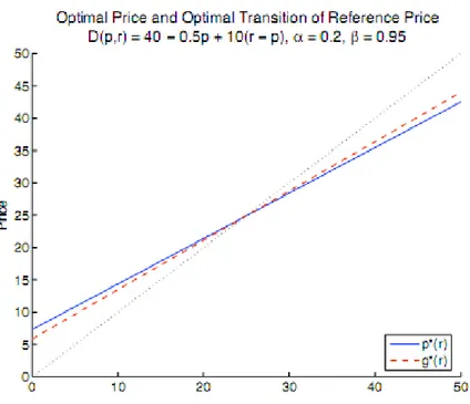
Figure 3.1 plots p⇤_(r) _{and g}⇤_(r)_{, and figure 3.2 shows how the optimal and reference}

prices converge to the steady state for two cases where r0 < r⇤⇤ and r0 > r⇤⇤.

Proposition 3 allows the extension of this result to asymmetric reference price eﬀect. Since the customers always perceive either a surcharge or a discount, the eﬀect of the reference price never switches between the two sides of the asymmetry.

3.4 Conclusion

In our current economic environment where internet made it easy to access the informa-tion, shoppers are becoming more and more sophisticated and aware of prices. In this chapter, we analyzed an optimal dynamic pricing model under repeated customer inter-actions for monopoly markets. Fibich et al. [14] solved for an explicit pricing formula in continuous-time, while claiming that an explicit solution in discrete-time is cumbersome. As a result, the optimal pricing policy they derived is a function of time, which is quite unnatural and diﬃcult to implement in practice. Our formula in discrete-time allowed us to derive a closed-form solution for the optimal pricing policy as a function of the state of the system, which is the current level of the reference price. This provides a more comprehensible tool to mangers, from which they can derive economic insights as well as implement the policy in practice.

(45)

3.4. Conclusion 35 The economics literature models competition in the market by assuming that the demand of a product is a function of it’s competitor’s price in addition to its own price. We intend to extend our result to a multiple-product scenario under competition. The concept of reference price would provide a diﬀerent framework for modeling competition where firms interact through their influence on the customers’ reference price.

(46)

(47)

Chapter 4

Dynamic Pricing for Multi-Products

with a Reference Price Eﬀect

Based on: S. Kachani, Y. Oumanar and N. Raissi, Dynamic Pricing for Multi-Products with Reference Price, Int. J. Applied. Math. Stat.

Abstract: This chapter addresses the problem of pricing for a retailer selling multiple products to a stream of repeated customers over an infinite time horizon. We propose a dynamic pricing model based on the concept of store-level reference price. We derive an optimal pricing policy and prove its monotone convergence in a monopoly context. We derive an analytical result for the optimal prices. Also, we address a comparison between the store-level and the product-level models and between optimal and myopic policies.

Keywords: Dynamic Pricing, Reference Price, Management Decision making, Dynamic Optimization.