Development of a new design method for the cross-section capacity of steel slender I-sections

© Caroline Arsenault, 2018

Development of a new design method for the

cross-section capacity of steel slender I-cross-sections

Mémoire

Caroline Arsenault

Maîtrise en génie civil - avec mémoire

Maître ès sciences (M. Sc.)

Development of a new design method for the

cross-section capacity of steel slender

I-sections

Master Thesis

Caroline Arsenault

Sous la codirection de:

Nicolas Boissonnade, Directeur de recherche

Mario Fafard, Codirecteur de recherche

iii

Résumé

Ce mémoire présente la recherche effectuée concernant le développement d’une nouvelle méthode de dimensionnement spécifiquement dédiée aux sections en acier en I très élancées par l’entremise de l’Overall Interaction Concept (O.I.C.). Le comportement en section est défini par deux comportements extrêmes, soit la résistance et l’instabilité pure. Les méthodes de calculs couramment utilisées dans les normes nécessitent d’abord de classer la section pour ensuite calculer les propriétés de la section efficace. Ces méthodes comportent quelques incohérences ainsi qu’un manque de précision. Une nouvelle méthode de dimensionnement qui considère la section entière – qui ne requiert donc plus de calculer les propriétés efficaces – et l’interaction entre les plaques peut et doit être développée. La considération des imperfections tant géométriques que matériels permet d’atteindre une plus grande précision, et l’utilisation d’outils numériques performants permet également d’augmenter l’efficacité des calculs.

L’Overall Interaction Concept permet de calculer rapidement la résistance en section en fonction de l’élancement relatif généralisée, au moyen de courbes d’interaction. L’objectif principal de cette maîtrise est donc d’adapter l’O.I.C. aux sections ouvertes en I très élancées, comme celles utilisées dans le domaine des ponts, soumises à des cas de chargement simples (compression pure ou flexion d’axe fort seulement).

Un modèle numérique a d’abord été développé en réalisant entre autres une étude de densité de maillage et des études sur les imperfections géométriques et matérielles à utiliser. Cette dernière étude doit être fait minutieusement et les choix effectués doivent être justifiés convenablement puisqu’aucune donnée expérimentale n’est disponible pour calibrer le modèle. Une fois le modèle fiable développé, une campagne numérique comptabilisant plus de 3500 simulations a été faite, permettant ainsi d’analyser l’effet de certains paramètres sur la résistance en section. Sur la base de ces simulations numériques, une proposition de méthode de dimensionnement a été faite en fonction des paramètres déterminants, c’est-à-dire le choix des contraintes résiduelles, du type de chargement et des propriétés géométriques géométrique de la section par l’entremise du paramètre μ. La formulation d’Ayrton-Perry a été adaptée pour définir les courbes d’interaction servant à prédire la résistance.

iv

En parallèle au développement de la méthode, des études ont été effectuées pour comparer les résultats obtenus pour la résistance en section selon les normes canadiennes, américaines et européennes avec les résultats obtenus numériquement. Ainsi, il a été possible d’observer la capacité d’amélioration des méthodes couramment utilisées tant en termes de précision que de simplicité.

v

Abstract

This dissertation presents research developments related to the design of very slender open steel sections through the Overall Interaction Concept (O.I.C.). The cross-sectional behaviour is defined by two extreme, ideal behaviours: pure resistance and pure instability. Methods used in the current standards need to classify the section, and, in the case of bridge sections, to calculate effective properties. This method presents some inconsistencies, as well as accuracy issues. A new design approach considering the whole section – and by that interaction between plates – was developed. By including the geometrical and material imperfections, more accuracy can be reached, and using numerical tools can increase the efficiency as well.

The Overall Interaction Concept allows to calculate fast the resistance of a cross-section by using a generalized relative slenderness, so-called interaction curves. The main aim of this master is to adapt the O.I.C. to very slender open I-sections subjected to simple load cases (major-axis bending moment and pure compression).

A numerical model has been developed by carry out mesh density study, and imperfections studies. This part had to be carefully detailed and assessed since no experimental data can be available to calibrate the numerical models. Once a reliable model was settled, a numerical campaign of more than 3500 simulations has been undertaken, allowing to analyse the effects of many key parameters. Based on these numerical simulations, design proposals were made as based on the identified governing parameters, i.e. the residual stresses pattern, load case and geometrical properties by means of newly-proposed parameter μ. An extension of the Ayrton-Perry formulation is finally used to define cross-section interaction curves.

Besides, systematic comparison with Canadian, American and European Standards are done with the results from numerical simulations allowing to observe the improvement capacity of the current methods, in terms of accuracy and simplicity.

vi

Table of Contents

List of Tables ... xvi

Notations ... xviii

Remerciements ... xxii

1 Introduction ... 1

1.1 Context ... 1

1.1.1 Use of the O.I.C. ... 2

1.2 Objectives of the master thesis ... 4

1.3 Methodology ... 4

2 State of the Art ... 6

2.1 Review about local buckling ... 6

2.1.1 Introduction ... 6

2.1.2 Brief historical review ... 6

2.1.3 European buckling curves ... 8

2.1.4 Concept of stability ... 11

2.1.5 Plate elastic buckling behaviour ... 13

2.1.6 Post buckling behaviour ... 16

2.1.7 Interaction between plates ... 18

2.2 Imperfections ... 20

vii

2.2.2 Material imperfections – Residual stresses ... 21

2.2.3 Geometrical imperfections ... 27

2.3 Current design methods ... 27

2.3.1 General overview ... 27

2.3.2 Cross-section resistance according to European Standard [8] ... 30

2.3.3 Cross-section resistance from Canadian Standard [27] ... 33

2.3.4 Cross-section resistance in American Standard [28] ... 37

2.3.5 Conclusion ... 39

3 Description of the F.E. models ... 43

3.1 Material behaviour ... 43

3.2 Residual stresses ... 44

3.3 Elements’ type ... 46

3.4 Geometrical imperfections ... 46

3.5 Support conditions and loading ... 47

4 Numerical Parametric Studies ... 50

4.1 Cross-sectional dimensions ... 50

4.2 Mesh density study ... 50

4.3 Geometrical imperfections studies ... 56

4.3.1 Local imperfections ... 57

4.3.2 Distortional imperfections ... 69

4.3.3 Final choice of imperfections ... 72

4.4 Material imperfections – Residual stresses influence ... 73

5 Identification of parameters governing the resistance ... 75

viii

5.2 Influence of plates slenderness – (h/w)/(b/t) ratio ... 76

5.3 Influence of web slenderness – (h/w) ratio ... 79

5.3.1 Validation of results ... 81

5.4 Influence of 𝒉 ∙ 𝒕𝒇𝟐𝒃 ∙ 𝒕𝒘𝟐 parameter ... 89

5.4.1 Influence of μ on welded sections with rolled flanges under bending moment 90 5.4.2 Influence of μ on welded sections with flame-cut flanges under bending .. 91

5.4.3 Influence of μ on welded sections with rolled flanges under compression 92 5.4.4 Influence of μ on welded sections with flame-cut flanges under compression 94 5.5 Conclusion ... 95

6 Proposed design curves ... 97

6.1 Sections under major-axis bending moment ... 97

6.2 Sections under pure compression ... 101

6.3 Summary ... 106

7 Accuracy and performance of propose – Comparison with design standards ... 108

7.1 Sections under major-axis bending moment ... 108

7.2 Sections under pure compression ... 112

7.3 Conclusion ... 114 8 Worked example ... 116 8.1 Introduction ... 116 8.2 Cross-section properties ... 116 8.3 Cross-section resistance ... 117 8.3.1 Canadian approach ... 117 8.3.2 Eurocode 3 approach ... 118

ix

8.3.3 O.I.C. approach ... 121

9 Conclusion and future developments ... 123

9.1 Main conclusions ... 123

9.2 Future developments ... 124

9.3 Wider context ... 125

10 References ... 126

11 Annexes ... 130

11.1 Annex 1: Comparison of the load ratio of the different standards ... 130

11.2 Annex 2: Comparison of the calculation methods between Canadian, American and European Standards ... 134

11.2.1 Canadian Standards ... 135

11.2.2 American Standards ... 136

11.2.3 European Standards ... 137

11.3 Annex 3: Impact of global buckling on the imperfections sub-study ... 139

11.4 Annex 4: First analysis of the key parameters ... 142

11.5 Annex 5: Comparison of critical load between FINELg and GTBUL, CUFSM and EBPlate ... 144

x

List of Figures

Figure 1 : Interaction curve ... 1

Figure 2 : Principles and application steps of the Overall Interaction Concept ... 2

Figure 3: First buckling curves proposal by ECCS ... 9

Figure 4: Buckling curves according to EC3 ... 11

Figure 5 : States of equilibrium ... 12

Figure 6: Instability by bifurcation ... 13

Figure 7 : Instability by divergence ... 13

Figure 8 : Post buckling behaviour [9] ... 14

Figure 9: Plate's local buckling ... 15

Figure 10 : Critical stresses distribution according to Von Kármán ... 17

Figure 11 : Residual stresses for a hot-rolled plate ... 21

Figure 12 : Residual stress for a welded plate ... 22

Figure 13 : Residual stresses for a flame-cut plate ... 22

Figure 14 : Welded section with flame-cut plates according to ECCS 1976 ... 23

Figure 15 : Residual stress pattern according to Barth and White [22] ... 24

Figure 16 : Residual stress pattern according to Chacon et al. [22] ... 24

Figure 17 : Residual stresses pattern according to Thiébaud [20] ... 25

Figure 18 : Residual stresses for welded sections with hot-rolled flanges (ECCS) ... 26

Figure 19 : Residual stresses pattern for welded sections with hot-rolled flanges (Gozzi) [24] ... 26

Figure 20 : Bending moment depending on the rotation & sections classification concept ... 28

xi

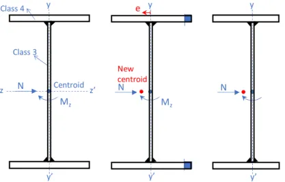
Figure 22: Additional major-axis bending moment due to load eccentricity ... 35

Figure 23: Additional minor-axis bending moment due to load eccentricity ... 36

Figure 24: Comparison between resistance values according to Canadian, American and European Standards ... 41

Figure 25 : Yun's constitutive law [30] ... 44

Figure 26 : Simplification of the ECCS's residual stresses pattern introduced in shell FE models ... 45

Figure 27: Auto-equilibrium residual stresses pattern magnified by 1017 _{for (a) welded} section with rolled plates and (b) welded section with flame-cut plates ... 46

Figure 28 : First eigenmode of a LBA ... 47

Figure 29: Improve: loading + support ... 48

Figure 30: Global instability for a simply supported section ... 49

Figure 31 : Four geometries considered ... 50

Figure 32 : Various mesh densities ... 51

Figure 33 : Mesh density studies, LBA results ... 52

Figure 34 : Initial geometrical imperfections used for mesh density study ... 53

Figure 35 : Effects of mesh density on GMNIA (a) accuracy, and (b) computation time 54 Figure 36 : Effects of mesh density on GMNIA (a) accuracy, and (b) computation time 55 Figure 37 : Geometrical imperfections (local) ... 56

Figure 38: Local imperfection with sinusoidal shape ... 57

Figure 39 : Different imperfections investigate (shape and amplitude) ... 59

Figure 40: Influence of imperfections’ amplitude ... 60

Figure 41: Results' comparison depending on the period ... 62

Figure 42: Member with length equal to a) two half-waves, and b) three half-waves ... 63

xii

Figure 44 : Lengths for imperfections study using first buckling mode shape ... 65

Figure 45: Results comparison depending on the amplitude using the first buckling mode shape ... 67

Figure 46: Sinusoidal vs eigenmode-conform imperfection shape ... 68

Figure 47: Influence of distortional imperfection amplitude ... 71

Figure 48: Final choice of imperfections (amplification factor: 10) ... 72

Figure 49: Effects of residual stresses on cross-sectional behaviour ... 73

Figure 50: Cross-sectional reduction factor depending on the slenderness for sections a) under pure compression, and b) under major-axis bending moment ... 75

Figure 51: Impact of plates' slenderness ratio on the reduction factor χL for welded sections with flame-cut flanges under pure compression ... 77

Figure 52: Impact of plates' slenderness ratio on the reduction factor χL for welded sections with flame-cut flanges under major-axis bending moment ... 78

Figure 53: Impact of web slenderness on the reduction factor χL for welded sections with flame-cut flanges under pure compression ... 79

Figure 54: Impact of web slenderness on the reduction factor χL for welded sections with flame-cut flanges under major-axis bending moment ... 80

Figure 55: Alternative lateral support modelling with 2 lateral supports ... 81

Figure 56: Curves for sections with continuous lateral support, and with only 2 lateral supports at 1/3 and 2/3 ... 82

Figure 57: Data entered in GBTUL ... 83

Figure 58: Example of dimensions and support data in EBPlate for section under compression ... 84

Figure 59: Elastic restraint generated by flanges ... 85

Figure 60: Plate's loading in compression in EBPlate ... 85

xiii

Figure 62: Dimensions and supports entered in EBPlate for section under bending moment ... 87 Figure 63: Plate's loading in bending moment in EBPlate ... 87 Figure 64 : Web instability mode for section under bending moment according to EBPlate ... 88 Figure 65: Influence of geometrical initial imperfection shape on χL values ... 88

Figure 66: Reduction factor χL depending on the cross-section slenderness λL for welded

section with rolled flanges – diverse values of μ under major-axis bending moment ... 90 Figure 67: Reduction factor χL depending on the cross-section slenderness λL for welded

section with flame-cut flanges – diverse values of μ under major-axis bending moment 91 Figure 68: Reduction factor χL depending on the cross-section slenderness λL for welded

section with rolled flanges – diverse values of μ under pure compression ... 92 Figure 69: Impact of ratio ℎ ∙ 𝑡𝑓3𝑏 ∙ 𝑡𝑤3 on the reduction factor χL for welded sections

with rolled flanges under pure compression ... 93 Figure 70: Impact of ratio ℎ ∙ 𝑡𝑓3𝑏 ∙ 𝑡𝑤3 on the reduction factor χL for welded sections

with rolled flanges under pure compression ... 94 Figure 71 : Reduction factor χL depending on the cross-section slenderness λL for welded

section with flame-cut flanges – diverse values of μ under pure compression ... 95 Figure 72 : Reduction factor χL depending on the cross-section slenderness λL and on μ

parameter for welded sections with rolled flanges under major-axis bending moment ... 97 Figure 73: Buckling curves depending on μ parameter for welded sections with rolled flanges under major-axis bending moment ... 98 Figure 74: Reduction factor χL depending on the cross-section slenderness λL and on the μ

parameter for welded sections with flame-cut flanges under major-axis bending moment ... 99 Figure 75: Buckling curves depending on the μ parameter for welded sections with flame-cut flanges under major-axis bending moment ... 100

xiv

Figure 76: Reduction factor χL depending on the cross-section slenderness λL and on the μ

parameter for welded sections with rolled flanges under pure compression ... 102

Figure 77: Buckling curves depending on the μ parameter for welded sections with rolled flanges under pure compression ... 103

Figure 78 : Reduction factor χL depending on the cross-section slenderness λL and on the μ parameter for welded sections with flame-cut flanges under pure compression ... 104

Figure 79: Buckling curves depending on the μ parameter for welded sections with flame-cut flanges under pure compression ... 105

Figure 80: Resistance comparison between standards and the proposed design model, with numerical simulations for welded sections with rolled flanges under major-axis bending moment ... 109

Figure 81 : Resistance comparison between standards and the proposed design model, with numerical simulations for welded sections with flame-cut flanges under major-axis bending moment ... 110

Figure 82: Resistance comparison between standards and the proposed design model, with numerical simulations for welded sections with rolled flanges under pure-compression ... 112

Figure 83 : Resistance comparison between standards and the proposed design model, with numerical simulations for welded sections with flame-cut flanges under pure-compression ... 113

Figure 84: Considered cross-section ... 116

Figure 85: Internal compression elements [12] ... 119

Figure 86: Cross-section dimensions ... 134

Figure 88: Effective area ... 138

Figure 88: Effects of imperfections' amplitude for simply supported sections ... 140

Figure 89: Effects of imperfections’ period for simply supported sections ... 141

xv

Figure 91: Influence of the yield stress on the interaction curve ... 142 Figure 92: Influence of the h/b ratio on the interaction curve ... 143 Figure 93: Impact of plates' slenderness ratio on the reduction factor χL for welded sections with a) rolled flanges, and b) flame-cut flanges ... 143

xvi

List of Tables

Table 1: Coefficients α and β for the first buckling curves proposal ... 9

Table 2: Imperfection factors used for EC3 buckling curves ... 11

Table 3: Values of k factor for various boundary conditions under compression and bending ... 16

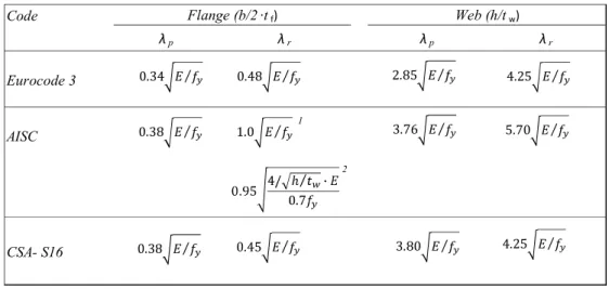
Table 4: Comparison of the width/thickness ratio for elements in bending ... 29

Table 5: Comparison of the width/thickness ratio for elements in compression ... 30

Table 6: Ayrton-Perry formula for sections under major-axis bending moment ... 106

Table 7: Ayrton-Perry formula for sections under pure compression ... 107

Table 8: Cross-section properties ... 117

Table 9: Summarize of buckling curves ... 124

Table 10: Comparison of the axial resistance between the three standards ... 130

Table 11: Cross-section properties for geometries under pure compression ... 131

Table 12: Comparison of the bending moment resistance between the three standards 132 Table 13: Cross-section properties for geometries under major-axis bending moment . 133 Table 14: Cross-section characteristics ... 134

Table 15: Loading and material properties ... 135

Table 16: Critical load of sections under compression with FINELg and GTBUL ... 144

Table 17 : Critical load of sections under compression with FINELg and CUFSM ... 144

Table 18 : Critical load of sections under bending moment with FINELg and CUFSM 144 Table 19: Critical load of sections under compression with FINELg and EBPlate ... 145

Table 20 : Critical load of sections under bending moment with FINELg and EBPlate 145 Table 21: Geometrical dimensions of sections used in the resistance comparison between F.E. method, standards and propose design model ... 146

xvii

Table 22: Results comparison between standards, F.E. results and propose model for welded sections with rolled flanges subjected to major-axis bending moment ... 147 Table 23: Results comparison between standards, F.E. results and propose model for welded sections with flame-cut flanges subjected to major-axis bending moment ... 148 Table 24: Results comparison between standards, F.E. results and propose model for welded sections with rolled flanges subjected to pure compression ... 149 Table 25: Results comparison between standards, F.E. results and propose model for welded sections with flame-cut flanges subjected to pure compression ... 150 Table 26: Ratios of the pure compression resistance according to Canadian, American and European Standards on the resistance obtained by F.E. method considering strain-hardening ... 151 Table 27: Ratios of the bending moment resistance according to Canadian, American and European Standards on the resistance obtained by F.E. method considering strain-hardening ... 152 Table 28 : Ratios of the pure compression resistance according to Canadian, American and European Standards on the resistance obtained by F.E. method without considering strain-hardening ... 153 Table 29 : Ratios of the bending moment resistance according to Canadian, American and European Standards on the resistance obtained by F.E. method without considering strain-hardening ... 154

xviii

Notations

Abbreviations

AISC American Institute of Steel Construction

EC3 Eurocode 3

ECCS European convention for constructional steelwork

EWM Effective Width Method

F.E. Finite Element

GMNIA Geometrically, materially nonlinear analysis with imperfections

LBA Linear Buckling Analysis

LTB Lateral torsional buckling

OIC Overall Interaction Concept

Latin letters

Acf Area of the compression flange

Aeff Effective area of the cross-section

Aw Web area

b Plate’s width

be Plate’s effective width

bfc width of the compression flange

Cf Factored compressive force

Cr Factored compressive resistance

dc Depth of the compression part of the web

E Young’s Modulus of elasticity

eNy Shift of the centroid of the effective area in the y-direction

xix

Fcr Critical stress

ƒu Material ultimate stress

ƒy Material yield stress

h web’s height

Iy Moment of inertia about the strong axis

Iz Moment of inertia about the weak axis

k Buckling coefficient

kc Coefficient for slender unstiffened elements

L Length

My, ed Design bending moment y-y axis (according to EC3)

Mz, ed Design bending moment z-z axis (according to EC3)

Mel Elastic bending moment

Mfx Factor bending moment about the x-axis (according to Canadian standard)

Mfy Factor bending moment about the y-axis (according to Canadian standard)

Mpl Plastic bending moment

Mr, AISC Factor moment resistance (according to American standard)

Mrx Factor moment resistance about the x-axis (according to Canadian standard)

Mry Factor moment resistance about the y-axis (according to Canadian standard)

Ned Design normal force (according to EC3)

NRd Design values of the resistance to normal force (according to EC3)

Pcr Euler critical load

Rb, L Resistance cross-section load multiplier

Rb, L +G Resistance cross-section load multiplier

xx Rcr, G Member critical load multiplier

Rpg Bending strength reduction factor

Rpl Plastic resistance load multiplier

S Elastic section modulus (according to Canadian standard)

Sxc Elastic section modulus referred to compression flange

t Thickness

tfc Thickness of the compression flange

tw Thickness of the web

w Deflection, web thickness

w0 Initial deflection

Wel Elastic section modulus (according to EC3)

Weff Effective section modulus

Weff, y min Minimum effective section modulus in the y-direction

Weff, z min Minimum effective section modulus in the z-direction

Zx Plastic section modulus (according to Canadian standard)

Greek letters

γM0 Partial factor for resistance of cross-sections

λ Slenderness parameter

λpf Limiting slenderness parameter for compact flange

λrf Limiting slenderness parameter for noncompact flange

λL Cross-section slenderness

λL+G Member slenderness considering local instability

𝜆 Plate slenderness

xxi

σc Compression stress

σcr Critical stress

σt Tension stress

ʋ Poisson’s ratio

Фs Resistance factor of steel (according to Canadian standard)

χL Cross-section reduction factor

xxii

Remerciements

J’aimerais tout d’abord remercier mon directeur de recherche, Nicolas Boissonnade pour m’avoir offert l’opportunité d’effectuer une maîtrise au sein de son équipe, mais également pour son écoute, son soutien et ses conseils. Merci d’avoir eu confiance en mes capacités, de m’avoir fourni les outils nécessaires pour mener à terme mon projet et pour développer un esprit critique. Les compétences acquises me seront assurément utile pour mon emploi en tant qu’ingénieure.

Merci également à mon co-directeur de recherche, Mario Fafard, pour son ses encouragements et son soutien financier. Son aide m’a particulièrement été bénéfique dans le cadre de mon stage effectué à Munich. Je le remercie également de m’avoir offert, il y a 3 ans de cela, un stage d’initiation à la recherche qui m’a donné envie de poursuivre au cycle supérieur.

J’aimerais également remercier Professeur Taras (Universität der Bundeswehr, München) pour son accueil et son aide lors de mon séjour. Cette expérience m’aura été bénéfique tant sur un plan personnel que professionnel.

Un énorme merci également à Lucile Gérard, collègue de travail et amie auprès de laquelle j’ai effectué ma maîtrise. Ton aide, ton support, ton écoute et tes conseils auront été précieux pour moi. Je te souhaite bonne chance pour la fin de ton doctorat!

Je remercie également ma famille, mes amis et bien-sûr mon conjoint, Antoine, pour leurs encouragements et leur patience à mon égard. Merci de m’avoir soutenu moralement et financièrement durant cette période.

Finalement, merci à mon employeur Tetra Tech, mais plus précisément à John Cafarelli pour ses encouragements à effectuer ma maîtrise et pour avoir pris part à ce projet.

1

1 Introduction

1.1 Context

The Overall Interaction Concept is a new alternative design method for steel members developed since 2012. Based on the resistance-instability interaction and the use of a generalized relative slenderness, this concept aims at offering an improved design method with more accuracy and simplicity. This approach also provides a framework for computer-assisted resistance predictions.

The O.I.C. evaluates the resistance of a section by means of an interaction curve (also called buckling curve). Once the relative slenderness (𝜆̅) is determined, the penalty factor (χ) which accounts for instability effects and the influence of imperfections, is applied to the pure plastic resistance of the cross-section. Obviously, this penalty factor cannot be more than 1.0. Figure 1 shows graphically these variables.

Figure 1 : Interaction curve

On this graph, the real behaviour illustrated shows that it is possible to obtain a factor χ greater than one. This is due to the plastic capacity which is calculated considering a plastique distribution (with constant constraint blocks), and no strain-hardening is considered. The O.I.C. uses advanced tools, and allows enhanced accuracy since it considers the geometrical and material imperfections.

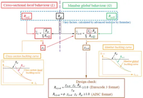
2

regarding steel design even though this method enhances inconsistencies and difficulties. In addition, for slender sections (class 4), the design rules rely on the Effective Width Method (E.W.M.) requires long and tedious calculations. These design methods may be over-conservative, as well as sometimes be unconservative. The O.I.C. has been developed to allow a faster and a more accurate resistance calculation method.

1.1.1 Use of the O.I.C.

Figure 2 : Principles and application steps of the Overall Interaction Concept

Figure 2 shows the steps for applying the Overall Interaction Concept. As illustrated on this figure, this approach addresses both the cross-section (local) and member (global) capacity. Even though the present study focuses on the cross-sectional behaviour, the O.I.C. way to deal with member resistance will be explained herein.

 Cross-section behaviour

o First, the plastic resistance named Rpl must be determine, and corresponds to the

factor by which the initial loading must be multiplied to reach the pure resistance limit. In this project, a MATLAB tool has been developed to facilitate the calculation.

o Then, the cross-sectional elastic critical load multiplier, noted Rcr,L, is obtained

3

using a linear buckling analysis (LBA) when finite element software is used, considering perfect elements, both geometrically and materially linear.

o Both values are used to determine the cross-sectional slenderness:

𝜆 = 𝑅 _𝑅

o The real resistance of the cross-section Rb,L can be obtained by hand calculations,

but it is preferable to use finite element software to reach a better precision (by including the plates interaction, material and geometrical imperfections, and possible strain-hardening influence as opposed to the effective width method). o The cross-section reduction factor, which reduces the plastic capacity due to

buckling effects, can then be calculated: 𝜒 = 𝑅 ,

𝑅  Member behaviour

o The member load multiplier Rcr,G is determined considering the global buckling

behaviour of an ideal elastic member.

o The cross-section reduction factor χL is applied to the plastic resistance Rpl to

obtain the member slenderness as influence by global instabilities as well:

𝜆̅ = 𝜒 ∙ 𝑅 _𝑅

,

o By performing a geometrically and materially nonlinear analysis with imperfections (GMNIA), the load ratio of the member Rb,L+G is obtained. Then,

the reduction factor considering the local-global coupled instabilities is obtained as follow:

𝜒 = ,

∙

As well as for the cross-section behaviour, formulas can be developed to enable rapid and efficient determination of real resistance of the member. However, in this report, this part will not be studied.

o Finally, the resistance χL+G is calculated as a function of λL+G . The cross-section

4

1.2 Objectives of the master thesis

The Overall Interaction Concept was already developed for hollow sections and hollow members. Following preliminary numerical tests on slender open sections, it has been established that the application of this new concept could and shall be adapted for this kind of sections.

It is not uncommon to see beams of very large dimensions used for bridge construction. They are usually constituted of welded plates forming a beam with stocky flanges and slender web. The very thin web plate is prone to undergo important local instabilities. Standards classify these sections as class 4 and provide formulae based on the EWM to calculate their resistance. As mentioned above, this method needs long and tedious calculations.

The main objective of this master is to adapt the O.I.C. to open sections used for bridges, i.e. welded sections of large dimensions. Herein, only doubly symmetric sections will be considered in this study. These sections require particular attention due to residual stresses generated by welding and flame-cut processes. Influence of plates buckling on the overall load-carrying capacity will be investigated as well as the geometrical and material imperfections. Leading parameters of the cross-section resistance shall then be identified. Then, a design approach according to the O.I.C will be proposed for class 4 sections with a yield limit of 355 MPa and 460 MPa, the most common values used for bridges. Even though sections used for bridges are mostly solicited in bending, two loading are also tested, namely axial compression N, and major-axis bending moment My.

1.3 Methodology

During the first step of the master, a review of literature has been done (Chapter 2 of this thesis), to get familiar with the O.I.C, its principles and theories, different method design and many tools, such as finite element software (FINELg), Zotero, FileZilla etc. It was also needed to be familiar with standards (European, Canadian and American). To compare the results, each standard has been programed in VBA Excel. In this way, it was possible to determine fast the cross-sectional resistance according to each standard.

Then, F.E. models have been built and each parameter used in has been validated. Sub-studies have been carried out, i.e. mesh density study and imperfections studies. Chapter 4 describes

5

the numerical models, as the material law used, geometrical imperfections – residual stresses patterns, elements’ type, geometrical imperfections and support conditions and loading. Chapter 5 is about the numerical parametric studies, to determine the right mesh density and geometrical imperfections to use. Identification of governing parameters has next be done in chapter 6 allowing to integrate all the parameters and to isolated those that govern the cross-section resistance calculation. When the lead parameters have been identified, a design approach according to the O.I.C. is proposed in chapter 7, and then compared to existing ones in chapter 8.

6

2 State of the Art

2.1 Review about local buckling

2.1.1 Introduction

The cross-section capacity depends on the width-to-thickness ratio of each plate composing the section. Instability increases with this ratio, and may consequently reduce resistance. Figure 1 showed that increasing the slenderness ratio induces a decrease in resistance. Sections studied here are classified as class 4, and, consequently, are more prone to suffer from local instabilities because of their high width-to-thickness ratio. These sections are acknowledged to do not reach their yield strength due to premature local buckling.

Since only cross-section behaviour is studied here, global instabilities will not be taken into account. Local buckling is the only instability considered. This phenomenon concerns plates loaded in their plane and involves plate deformations only. It can occur in the flanges or in the web due to compression stresses. This local buckling occurs when the elastic critical buckling stress is reached for a materially and geometrically perfect plate.

2.1.2 Brief historical review

Jacob Bernoulli (1654-1705), Swiss mathematician and physicist, is at the origin of the theory according to which the curvature of an elastic beam at each point is proportional to the bending moment at that point. Other mathematicians (especially Euler) used this assumption in their work about elastic curves [1].

The Swiss mathematician Leonhard Euler (1707-1783) contributed to the strength of material by focusing mainly on the geometrical forms of elastic curves. Bernoulli’s theory was accepted by Euler without much discussion. With this assumption, he studied the curvature response of slender elastic bars under different loading conditions [1]. He published in 1744 the famous critical load formula under the title Methodus inveniendi lineas curvas maximi minimive proprietate gaudentes [2]. His contribution to structural engineering is unprecedented. He was the first to establish a formula which determines the critical buckling load of a column [3]. Euler’s original work concerned the determination of the buckling load of a column fixed at the bottom and free at the top under a centrally axial compression load

7

[4]. However, the Euler load consider only a geometrically and materially perfect column, thus no imperfection is included in his model. His formula is shown in Equation (1).

2 cr E I P L     (1)

Euler assumed that a column under an axial load would not suffer from deflections if the load is below the critical value. To obtain this famous equation, Euler introduced the modulus E, called at this time the modulus of extension, which characterize the material [5].

Thomas Young (1773-1829) took a part of the Euler and the Bernoullis’ work [5]. He established that the amplitude of the modulus, now called Young’s modulus, is independent of the cross-sectional area. He noticed and brought to attention the fact that a longitudinal deformation is always accompanied by a lateral change of dimensions. He observed that the Hooke’s law, according to which there is a linear relationship between stress and deformation, is applicable only up to a certain limit. Beyond this limit, a proportion of the deformation is permanent and inelastic [1]. He is also the first to prove that the real columns behaviour is affected by geometrical imperfections, by the initial load eccentricity, and by the initial curvature of the bar. He also states that the buckling phenomenon is affected by the inhomogeneity of the material [6]. Additionally, he is the first to introduce the second order moment notion, obtained by multiplying the first order moment by a coefficient K, so

that II I

M  K M . For a simply-supported bar with an initial sinusoidal curvature of amplitude e0, and for a straight column under an axial load with an eccentricity e0, the

coefficients K are obtained respectively by Equations (2) and (3). However, his model did not get the deserved attention during several following years.

1 1 cr K N N   (2) 1 cos 2 _cr K N N



Friedrich Engesser (1848-1931) extended Euler’s formula for non-linear material by using the tangent modulus approach. Thus, he could determine the critical stress for bars of

8

structural steel beyond the elastic limit. He was also the first to work with the theory of buckling of built-up columns [1]. F.S. Jasinsky (1856-1899) was the first to investigate the stability of diagonals in compression and to evaluate the strengthening provided by the diagonals in truss systems. His main work was related to the difficulties encountered in bridge engineering. Contrary to Engesser, he proposed rather a reduced modulus, between the tangent modulus and the elasticity modulus E. In return, Theodore Von Kármán showed in 1910 that the reduced modulus of a rectangular section is given by Equation (4).





Ayrton-Perry formulae (1886) considers imperfections and is the one currently used by the Eurocode [7] and many other standards worldwide. Even if the inelastic reserve is included, the strain-hardening is not considered by Ayrton-Perry.

Stability principles evolved considerably since Euler’s proposal. A new simpler and accurate method could probably be developed for current standards, which would consider the whole cross-section, the interaction between plates of girder and the imperfections.

2.1.3 European buckling curves

In 1955, the European convention for constructional steelwork (ECCS) was created. The ECCS was initially formed by eight countries with the main objective to relaunch the use of steel in constructions after the Second World War. From 1960, The ECCS attempted to standardize methods used in the European Standards at the time. The ECCS has established a wide theoretical and experimental research council, which proposed in 1970 three buckling curves associated to different cross-section shapes and considering structural and geometrical heterogeneities. Those curves provide the ultimate load of a column depending on its relative slenderness 𝜆̅ [6]. 2 2 ₂ 2 1 (0.5 ) (0.5 ) N               (5)

9

Table 1: Coefficients α and β for the first buckling curves proposal

Figure 3 shows the three initial curves proposed by the ECCS in 1970, which represent the reduction buckling factor 𝑁 depending on the relative slenderness 𝜆̅. The European buckling curves are non-dimensional, since it has been observed that a moderate variation of the yield stress does not change significantly the behaviour. Values of the reduction factor 𝑁, and of the relative slenderness 𝜆̅ are obtained with following Equations (6) and (7).

K r N











In these previous equations, σK and σr correspond to the critical buckling stress, and to the

yield stress of the material, respectively, while 𝜆 and 𝜆 correspond to the bar slenderness in the considered buckling plane, and to the so-called “Euler slenderness” (= 𝜋 ∙ 𝐸 𝜎⁄ ). [6]

Figure 3: First buckling curves proposal by ECCS

Curve α β a 0.514 -0.795 b 0.554 -0.738 c 0.532 -0.377 Reduced slenderness  0.0 0.2 0.4 0.6 0.8 1.0 1.2 1.4 1.6 1.8 2.0 2.2 2.4 2.6 2.8 3.0 0.0 0.1 0.2 0.3 0.4 0.5 0.6 0.7 0.8 0.9 1.0 1.1 a b c 𝑁

10

On the other hand, it has been established that when the relative slenderness is low, strain hardening predominates on the buckling. Thus, a plateau was introduced at the beginning of the curves until a given slenderness. Furthermore, the initial curves considered only steel grades Fe 360 and Fe 510 (S235 and S355 formally denoted now), with plate’s thickness lower than 40 mm. Nowadays, it is common to use higher steel grades with flange’s thickness of more than 40 mm. New curves considering these factors had to be established. [6] Few years later, in response to several critics, five new curves were proposed. This proposal made in 1976 includes a plateau for relative slenderness lower than 0.2. Many studies, research investigations, experimentations, and proposals have been made to get the current methods used in the EC3. [6]

In the European Standard, the buckling curves depend on the section geometry and the fabrication process. Different buckling curves are used for hot-rolled and welded I-sections, for cold-formed and hot-rolled hollow sections, etc. The yield stress and the axis of buckling have an impact on the choice of the curve as well. Those curves exhibit the reduction factor χ in function of the relative slenderness 𝜆̅. Equation (8) shows the relation between the two parameters. [8] 2 2 1 1.0         (8)

In the previous equation, parameter 𝜙 is obtained with Equation (9).

2

0.5 1 ( 0.2)

    _    _ (9)

The relative slenderness is calculated differently depending on the section classification. For sections class 1, 2 or 3, the relative slenderness is calculated with Equation (10), i.e. using the whole section, while for a class 4, effective area is used, as shown in Equation (11).

y cr A f N





11

coefficient are shown in Table 2 depending on the curve letter. [8]

Table 2: Imperfection factors used for EC3 buckling curves

The choice of the curve depends on the steel grade, the geometry, the fabrication process, and the axis of bending. A table in the EC3 prescribes the choice to make. From Equation (8), curves are plotted on Figure 4, for slenderness from 0 to 3. Contrary to the first proposal, there are five curves, with plateaus for slenderness lower than 0.2. So, for relative slenderness lower than 0.2, buckling effects can be neglected and only cross-sectional verifications apply.

Figure 4: Buckling curves according to EC3

2.1.4 Concept of stability

Stability is a widely used concept in steel structures. It is a key parameter which often governs in the ultimate resistance calculation of a compressed section to the detriment of the sectional resistance. In this part, the concept of instability will be presented with a ball analogy as shown in Figure 5. Curve a0 a b c d α 0.13 0.21 0.34 0.49 0.76 Reduced slenderness  0.0 0.2 0.4 0.6 0.8 1.0 1.2 1.4 1.6 1.8 2.0 2.2 2.4 2.6 2.8 3.0 R ed uc ed c oe ff ic ie nt  0.0 0.1 0.2 0.3 0.4 0.5 0.6 0.7 0.8 0.9 1.0 1.1 a₀ a b c d

12

Figure 5 : States of equilibrium

On the left drawing, the ball is in an equilibrium state. If an external load is applied on it, it will move but it will come back to its initial state when the perturbation will be removed. This is called the stable equilibrium. Analogously, a bar under axial compression load which generates a small displacement is in an equilibrium state if it returns to its initial position when the load is removed.

The second drawing shows a ball in a neutral equilibrium. If a perturbation is applied, the ball will move, but the removal of the disturbance does not bring the ball back to its original location. This is the principle that applies to a bar at its critical load. When the load is removed, the bar will remain its position which is its new state of equilibrium. So, if the column is subjected to any external influence which generates a small displacement which is then removed, the column will return to this new equilibrium state.

Finally, the third drawing shows an unstable equilibrium. A lesser effort applied to the ball will generate an important displacement, and the ball will not return to its initial position when the perturbation is removed. Unlike the neutral state, the ball will not find a new equilibrium state. Similarly, a column under a compression load greater than the critical load will undergo a large deformation and will make the system unstable.

For an idealized column, instability phenomenon by bifurcation is illustrated in Figure 6. The point B on the graph corresponds to the bifurcation point. The two red lines represent the equilibrium conditions, the vertical one is the initial state and the horizontal one corresponds to the deformed structure. Up to point B, the structure will return to its initial position when the load is removed, while a permanent deformation is observed at point B if the plastic state is reached. In this case, the structure remains in an equilibrium state, which is not the case of a load exceeding point B.

13

Figure 6: Instability by bifurcation

Considering unavoidable geometrical imperfections, a real structural element does not buckle by bifurcation, but rather by divergence. Before the beginning of the loading, there is already a deflection due to initial imperfections w0. Then, from the beginning of the loading,

deflections increase. The curve becomes asymptotic to the critical load at the final stage and will never reach the critical value because of the residual stresses [9].

Figure 7 : Instability by divergence

2.1.5 Plate elastic buckling behaviour

Counter to member instabilities, elastic buckling in plate does not necessarily coincides with failure of the plate (see Figure 8). Indeed, after local buckling occurs, the plate continues to resist due to membrane effects and stress redistributions. Fibers parallel to the load are in compression while the perpendicular ones are in tension. Given that only compression generates buckling, the tension fibers act as springs and prevent buckling of those compress.

Axial load P Pcr Deflection w Neutral equilibrium P = Pcr Stable equilibrium P < Pcr Unstable equilibrium P > Pcr O B Bifurcation point

14

The plate must be supported on at least one edge parallel to the load application to enhance this additional strength. Otherwise, the plate would behave like a column in compression and would fail by global buckling. After the load on the plate has reached its theoretical critical load, the stress distribution is no longer uniform along the section [10].

Figure 8 : Post buckling behaviour [9]

The first drawing of Figure 9 shows a plate which is four sides supported and uniformly loaded in compression in x-direction. The second drawing shows fibers in compression parallel to the loading and fibers in tension perpendicular to the loading. Until the critical load is reached, the stresses distribution is uniform. The third drawing, shows the stresses distribution once the critical load is reached. The bowing effect in the central zone makes the distribution no longer uniform. The compression stress decreases in the middle of the plate and tends to increase in the portions close to the supported edges since they are the stiffest edges in a buckled plate. Therefore, the tensile membrane action and the stress redistribution enable the plate to develop significant postbuckling strength [11].

15

Figure 9: Plate's local buckling

The critical buckling stress corresponds to the stress under which the plate will begin to deform out of its loaded plan. It does not depend on the yield stress but on the geometry (slenderness b/t). According to the linear theory of local buckling [10], the differential equation for a buckled plate uniformly compressed in the x-direction and supported on its four edges is:

4 4 4 2 2 4 2 2 4 3 2 12 (1 ) 2 _x w w w w N x x y y E t x   _{ }  _ _{ }   _{ }       (12)

Sinusoidal solution satisfies this equation. The deflection w depends on the number of half-waves in the x-direction (m) and in the y-direction (n).

1,2,3... 1,2,3... sin sin mn m n m x n x w w a b       

 

From solving the last equations, the elastic critical buckling stress is:

2 2 , _{12 (1} 2₎ cr P E t k b







In this equation, k corresponds to the buckling coefficient which depends on the boundary conditions. This parameter depends on the number of half-waves m and n, and the plate aspect ratio a/b. 2 2 n a b k m m b a   _    _   (15)

For a plate in a girder, the aspect ratio is generally large, and the minimum value of k can be used. For the flanges, which can be considered as a plate supported along one edge, the

16

coefficient k is equal to 0.43. For the web, which is supported on both extremities by the flanges, a coefficient k of 4.0 is taken [12]. Table 3 gives values of the buckling coefficient k for plate under compression and bending, for different boundary conditions. As shown, this parameter varies considerably depending on the boundary conditions and stress distribution. These values are used in the current standards [13].

Table 3: Values of k factor for various boundary conditions under compression and bending

2.1.6 Post buckling behaviour

17

stress distribution was uniform. Non-linear calculations are necessary to analyze a plate in its post critical domain shown in Figure 8. The stress distribution becomes more complex (see third drawing in Figure 9) and more difficult to analyze. The dashed line in Figure 8 represents the behaviour of an imperfect plate with initial deflection w0 whereas the solid line

enhances the response of a perfect plate. Even though there is a large post-critical reserve, which is ignored by the linear plate buckling theory and standards ignore this gain in resistance which constitutes a fundamental weakness [9]. Actually, even if the buckling occurs, the plate still resists, which is ignored by this theory.

According to the von Kármán approach, the critical stress distribution of a plate under compression, which is non-linear, can be replaced by a uniform stress block over a certain effective width be (see Figure 10).

Figure 10 : Critical stresses distribution according to Von Kármán

Von Kármán’s hypothesis assumes that the critical buckling stress of a plate with a reduced width should be equal to the yield stress [14]:









2 ₂ 2 2

2 2

, , _{12 1} 2 _{12 1} 2 ,

cr P eff cr P y

eff eff eff

E t E t b b f b b b b

















Geometrical and material imperfections are not considered in the von Kármán approach, which is not accurate because both imperfections induce early local buckling which occurs

18

before reaching the critical buckling stress. Therefore, Winter [14] proposed an alternative formula for defining the effective width for a compressed articulated plate as based on test data done on real (small) plates:

0.22 1 eff p p b b       _{ }   (18) where , y p cr P f    (19)

This theory represents the basis of the effective width method which is nowadays used in standards. In EC3 part 1-5 [12], formulas known as Winter modified formulas are suggested.

2.1.7 Interaction between plates

In the current standards, section classification is based on the properties of individual plate elements, and follows an “individual plate rule”. In this way, each plate must be classified, and the worst one is retained. Web and flange of I-sections are considered as a plate simply-supported along four edges, and as a plate simply-simply-supported along three edges [15]. The slenderest element determines the section classification. Even if it is ignored by the standards, there is a considerable interaction between plates constituting the section. The more stable elements have the capacity to provide assistance to the less stable ones. Following his experimental study, Cheng concluded that the web-flange interaction of H-section steel beam-columns has a significant influence on the cross-sectional behaviour [16]. For section subjected to axial compression, it has been established that the ultimate load decreases with increasing the plates slenderness. However, at a given ratio, the relation between the ultimate load and the slenderness is less significant for both flanges and web. Then, plate buckling depends on the slenderness of the adjacent plates [17]. Flanges provide rotational restraints which may have a noticeable effect on the buckling of the web.

Usually, the critical local buckling stress of an assembly of plates may be taken as the smallest value of critical stress composing the section. This approach provides a conservative value for the section’s critical stress, if the slenderness of elements varies widely. Indeed, no rotational restraints are considered at the junctions of the web and the flanges [18].

19

Bleich presented a different way to calculate to critical stress of a girder, which considers the whole section and the interaction between plates [19]. From the critical buckling stress equation (Equation (14)), the limit case where the flange and the web buckle simultaneously can be determined. 2 2 2 2 2 2 0.425 4.0 12 (1 ) 12 (1 ) f w f w t t E E b h            _{ } _ _   _{ }       (20) 2 2 0.425 f 4.0 w f w t t b h     _ _        (21) 0.425 0.326 4.0 f w w f b t h t     (22)

From Equation (20) to Equation (22), it has been established that for a ratio b t h t_f  _{w w} _f

lower than 0.326, flanges support the web and the buckling stress of the cross-section under pure compression is leaded by the web, and given by the Equation (23).

2 2 , _{12 (1} 2₎ w cr L w w t E k h         _{ }   _{ } (23)

However, buckling coefficient kw is given by the following Equation [19]:

2 2 2 10 3 w w k    _  _     (24)

As shown on the previous equation, the buckling coefficient depends on the coefficient of restraint denoted ξw, and obtained with Equation (25) [19].

3 2 0.16 0.0056 4.0 1 0.425 w f w w f _{f w} w f h b t t _{b t} h t



In contrast to the standards, hw corresponds to the distance between the middle line of the

flanges, and bf to the distance between the middle line of the web to the edge of the flange.

20

lower than 0.326, web is considered supported by the flanges and the critical stress of the cross-section considered the impact of both web and flanges.

If the ratio b t h t_f  _{w w} _f is greater than 0.326, this means that flanges are supported by the web and the buckling stress of the whole cross-section can be calculated with Equation (26), Equation (27) and Equation (28).

2 2 , _{12 (1} 2₎ f cr L f f t E k b         _ _   _{ } (26) 2 2 0.65 3 4 f k



In the previous equations, 𝜎 _, provides the critical stress of the cross-section, while ξ provides rather the restraint coefficient.

2.2 Imperfections

2.2.1 Introduction

Manufacturing processes generate geometrical and material imperfections. Those identified as geometrical imperfections constitute initial deformations of the plates forming the section. The non-linearity of the plates response induces a modification in the structural response of the elements. Material imperfections induce initial stresses in plates of the section. The structural behaviour is thus disturbed because of the premature yielding of the steel in certain areas. However, by altering the rigidity of the material, the capacity of the section may be reduced due to the risk of instability [20].

It is essential to take into account their influence in the finite element (F.E.) models. But first, it is imperative to understand their origin and to know different models used to represent them.

21

2.2.2 Material imperfections – Residual stresses

2.2.2.1 Plate’s residual stresses patterns

Residual stress is an existing state of stress in material under no external load and that arise from fabrication process. Here, only thermal residual stresses are considered. It depends on the fabrication process which generates uneven cooling along the thickness. The part of the material which cools first is in residual compression, while the last part to cool is in residual tension [21]. Thus, areas the most affected by heat (for example, near to the flame-cut area or to the welding) are in tension. Once manufacturing is completed, the residual stresses within a plate are self-equilibrated which means that there is no additional force before loading. They influence the cross-section behavior by creating premature local yielding which leads to a loss stiffness and a reduction load carrying capacity.

Residual stresses vary depending on the fabrication process. Bridges sections here studied are constituted of three plates (hot-rolled or flame-cut) welded. Depending on the manufacturing of each plate, the residual stresses pattern will differ.

For a hot-rolled plate, a simple residual stress pattern commonly used is shown in Figure 11. It consists in a parabolic distribution with compression areas at the ends and with a tension area in the middle. Amplitude of stresses depends on two parameters, i.e. width to thickness ratio and the perimeter over cross-sectional area ratio [21].

Figure 11 : Residual stresses for a hot-rolled plate

Another residual stresses pattern for plate with a weld is shown in Figure 12. As mentioned previously, welding induces a tension stress to the most thermally affected area (near the welding). It is a simple stress distribution idealized through rectangular blocks. Residual stresses on a welded section can be analysed as an assembly of plates which residual stresses are all self-equilibrated [21].

22

Figure 12 : Residual stress for a welded plate

Flame-cutting is a thermal cutting method used to cut large steel plates. Material is heated locally by the flame which thermally affects an area. This method results in a residual tension stresses on a width cf in the plate with an intensity equal to a proportion of the yield stress of

the material fy. A residual compression stress is induced in the remainder of the plate to

achieve a state of internal equilibrium.

Figure 13 : Residual stresses for a flame-cut plate

2.2.2.2 Section’s residual stresses patterns

Bridge girders typically consist in two types of welded sections, those with flame-cut flanges and those with hot-rolled flanges.

Typical residual stresses patterns of flame-cut and hot-rolled flanges consist in alternate tension/compression constant stress blocks. Due to flame-cut and welding operations, there are tension areas reaching a proportion of fy. The remaining parts of the flange reach a

compressive stress which allows the plate to be in an equilibrium state. 2.2.2.2.1 Flame-cut flanges

According to ECCS [21], the ends of the plates flame-cut obtained by flame-cutting, reach a tension stress equal to the yield stress as well as for the welded area at the flange-web

σr Cf Cf b t σr σc

23

junctions. Remaining parts of the plates reach a specific compression stress allowing to each plate to be in self equilibrium.

Figure 14 : Welded section with flame-cut plates according to ECCS 1976

Figure 14 showsthe residual stress pattern suggested by the ECCS for a welded section with flame-cut plates. The width cf at the flange ends corresponds to the area affected by the

flame-cutting. This value is obtained by:

110 f y t c f   (29)

The width cfw over which the web is in tension is given by:

12000

p A

c

f

t

 







The definition of each parameter included in the two previous formulas are provided by [22]. However, various authors have proposed alternatives to the ECCS’s pattern. Barth and White suggested a simplification of this model (Figure 15) [22]. Contrary to the ECCS, Barth and White proposal definition of the width of each rectangular block depends on the dimensions of the web and flanges. In addition, as shown in Figure 15, the maximum intensity of the tensile stress does not reach the yield limit fy.

fy fy fy Cf Cf 2C2 C fw f y C fw f y

24

Figure 15 : Residual stress pattern according to Barth and White [22]

Chacon et al. proposed their own model only to provide a simplified one for numerical and modeling purposes (Figure 16) [22]. Their model differs from the ECCS one by the width of the rectangular stress blocks and by the magnitude of those blocks. Indeed, width depends on the dimensions of the section and block magnitude is lower than the yield stress.

Figure 16 : Residual stress pattern according to Chacon et al. [22]

The residual stresses pattern shown in Figure 17 come from Thiébaud’s thesis [20]. Ends of the flanges reach a tension stress equal to 0.20 times the yield limit over a width of bf/20. At

the welded area, the tension stress reaches 0.68 fy along a 2 bf/20 width. The rest of the flange

is in compression to be in a state of auto-equilibrium. On the web, welding affects an area

0.18fy 0.6 3f y 0.18fy 0.6 3f y -0 .0 7f y -0.17fy -0.17fy 0.33fy 0.1b 0.3b 0.2b 0.3b 0.1b 0.05hw 0.9hw 0.05hw 0.18fy 0.6 3f y 0.18fy 0.6 3f y -0 .1 5f y -0.20fy -0.20fy 0.33fy b/20 9b/40 9b/20 9b/40 b/20 0.1hw 0.8hw 0.1hw

25

with a width of hw/20. The tension stress at these points reaches 0.63 fy, and the compression

one a value of 0.11 fy. Thus, each plate is in an equilibrium state.

Figure 17 : Residual stresses pattern according to Thiébaud [20]

2.2.2.2.2 Rolled flanges

Contrary to alternative models of residual stresses for welded sections with flame-cut plates, those with hot-rolled flanges reach the yield stress in tension. In addition, there is no tension block at the flange’s ends.

Figure 18 shows a residual stresses pattern applicable to welded sections with hot-rolled flanges provided by ECCS [23]. This pattern consists of trapezoidal shapes with magnitudes in tension area equal to the yield stress fy. Indeed, the flange-web junction is affected by the

weld which results in a tension stress in this area. The remaining of the flange is in compression to ensure equilibrium of the plate.

0.20fy Cf 2Cf C fw 0.6 3f y C fw Cf 0.20fy 0.6 3f y -0 .0 7f y -0.11fy -0.11fy 0.68fy

26

Figure 18 : Residual stresses for welded sections with hot-rolled flanges (ECCS)

In the ECCS pattern (Figure 18), the widths of tension and compression areas depend on the width b of the flange, depth of the web h, and thickness of the flanges t. Transition between tension and compression is linear.

In his doctoral thesis, Gozzi proposed a simpler alternative model [24]. Trapezoidal shapes are replaced by rectangular ones. Width of each block depends on the thickness of the flange and the web. The maximal tension stress is still equal to the elastic limit. The magnitude of the stress in compression is chosen to fulfil the stress equilibrium within each plate.

Figure 19 : Residual stresses pattern for welded sections with hot-rolled flanges (Gozzi) [24]

fy 0.0 75 h f y 0.075b 0.125b -0.25fy 0.1 25 h -0 .2 5f y fy f y 2.25tf σc σ c 2.2 5t w f y 2.2 5t w

27

2.2.3 Geometrical imperfections

2.2.3.1 Local imperfections

Local imperfections exist in every plate, since it is impossible to obtain a plate perfectly perfect.

2.2.3.2 Distortional imperfections

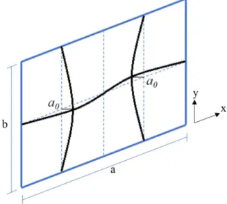
Distortional imperfections correspond to a translation of one flange while the one at the other end stay fixed. After having looked for on previous works and publications on this subject, it was agreed that there is not much information. So, it would be relevant to study their impacts and to determine a reference value for amplitude used for numerical tests.

2.2.3.3 Imperfection tolerances

Imperfections need to be included in the F.E. models. Annex C of EC3 part 1-5, recommends a magnitude of the local imperfection of a/200, where a is the plate’s width [12]. It is also recommended to use a shape of imperfections corresponding to the buckling shape. When combining of imperfections is necessary (geometrical or material), the leading imperfection must be fully considered, and the others may be reduced to 70% of their amplitude.

According to the CSA G40.20-13 (General requirements for rolled or welded structural quality steel/Structural quality steel), no matter the depth of the section, a lack of flatness up to A/150 is acceptable, where A correspond to the depth of the section [25].

2.3 Current design methods

2.3.1 General overview

Standards determine the cross-sectional resistance according to a classification system. For a section under compression, there are two different classes of sections, i.e. compact (classes 1, 2 or 3) and slender (class 4). For a section subjected to bending, there are four classes of sections for European and Canadian Standards, and only three for the American one. The class of a section depends on the slenderness of each plate subjected to compression that constitutes the section. The slenderness of a plate is determined by its width-to-thickness ratio. The plate with the most critical slenderness will dictate the classification of the section. Although very similar, each standard has their own limit values of slenderness in