The simulated detection of low-mass companions with GENIE

The simulated detection of low-mass companions with GENIE

Roland den Hartog

,

O. Absil

, P. Gondoin

, L. D’Arcio

, P. Fabry

, L. Kaltenegger

, R. Wilhelm

,

P. Gitton

, F. Puech

, M. Fridlund

1

Science Payloads and Advanced Concepts Office, European Space Agency, ESTEC,

P.O. Box 299, NL-2200AG Noordwijk, The Netherlands

2

Institut d'Astrophysique et de Géophysique, Université de Liège, Belgium

3

European Southern Observatory, Garching bei München, Germany

ABSTRACT

The prime objective of GENIE (Ground-based European Nulling Interferometry Experiment) is to obtain experience with the design, construction and operation of an IR nulling interferometer, as a preparation for the DARWIN / TPF mission. In this context, the detection of a planet orbiting another star would provide an excellent demonstration of nulling interferometry. Doing this through the atmosphere, however, is a formidable task. In this paper we assess the prospects of detecting with nulling interferometry on ESO’s VLTI, low-mass companions in orbit around their parent stars. With the GENIE science simulator (GENIEsim) we can model realistic detection scenarios for the GENIE instrument operating in the VLTI environment, and derive detailed requirements on control-loop performance, IR background subtraction and the accuracy of the photometry calibration. We analyse the technical feasibility of several scenarios for the detection of low-mass companions in the L’-band.

Keywords: Nulling interferometry, Bracewell array, planet detection, DARWIN, GENIE, OPD modulation

1. INTRODUCTION

GENIE, the Ground-based European Nulling Interferometry Experiment, is a precursor study carried out in the context of the Darwin Technical Research Programme of the European Space Agency. GENIE is a collaboration between ESO and ESA, and intended for commissioning at the VLTI site on mount Paranal in Chile in 2008. ESA has initiated two definition studies with Alcatel (France) and EADS Astrium (Germany), to be completed in December 2004. One of the intermediate outcomes of these studies has been the unanimous choice for the L’ -band (3.5 − 4.1 µm) as the operating band for GENIE.

The main objective of GENIE is to obtain experience with the design, construction and operation of an IR nulling interferometer using techniques and concept which are representative for the Darwin / TPF mission.1,2 The primary goal is therefore to demonstrate the feasibility of deep nulling, by recording nulls deeper than 1000. The second goal is to prepare the Darwin mission by screening the Darwin target stars which are accessible from the VLTI for the presence of exo-zodiacal dust down to a level of 10 to 20 times the local zodiacal cloud. In the context of the Darwin mission, the detection of a planet orbiting another star would provide an excellent demonstration of nulling interferometry.3 These goals are actually merely a tip of the iceberg regarding the full scientific potential of GENIE.1,4,5 It is therefore the intention to operate GENIE as a general user-instrument at ESO VLTI.

In order to assess GENIE’s potential performance, to assist in the requirements definition and to prepare science studies, ESA has, in collaboration with the University of Liege, developed a GENIE science simulator, GENIEsim.6 With this simulator we revisit the prospects of detecting low-mass companions (i.e hot Jupiters and brighter) around a parent star. In a previous study3 we found that although it is possible to obtain useful signal-to-noise ratios on the planetary signal in an hour of integration, the planetary signal is so much smaller than the contributions due to leakage and IR background

Further author information:

that the requirements on photometric calibration of the output signal would become unreasonable. In this paper we demonstrate that this problem can be overcome with an additional technique called OPD modulation.7

2. GENIESIM

The objectives of the science simulator are manifold. The main purpose is to estimate GENIE performance as well as possible and to assess the impact of the atmosphere and t he VLTI environment.8 This helps us to quantify specifications, define required GENIE functionality, operation and calibration modes, and select between different proposed concepts and/or designs. By simulation of observational scenarios we can test data reduction and analysis procedures. And finally, since all our relevant knowledge is embedded in the code, the Geniesim code is also a means to distribute our knowledge of Genie to the wider scientific community.

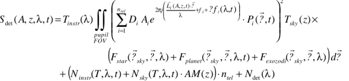
The GENIEsim inputs consist of specifications for the interferometer configuration, target source, observational scenario, atmospheric conditions, detector and control loop performance. The outputs are a series of detected photo-electron numbers (for constructive and destructive interference modes) as a function of position in the sky (A, z) wavelength λ and time t, conform the following expression,

(1.)

where Tinstr is the instrumental transmission, ntel is the number of telescopes, Di are the telescope diameters, Ai the

normalization factors for beam combination, Li are the position vectors of the telescopes projected onto the sky, ϕi the

fixed phase delays, ∆ϕi the errors on the phases due to atmospheric and environmental perturbations, Pi the intensity and

fiber coupling fluctuations, Tsky is the atmospheric transmission, Fstar, Fplanet and Fexozodi, the signals of respectively the

.

Figure 1. Illustration of the model for the control loops used in GENIEsim. Apart from the standard ingredients, sensor, controller

and actuator, latency and digital-to-analog conversion are taken into account.

(

)

(

(

,

,

)

(

,

,

)

(

)

)

(

)

)

,

,

(

)

,

,

,

(

)

,

,

(

)

(

)

,

(

)

(

)

,

,

,

(

λ

λ

λ

λ

λ

λ

λ

λ

N

n

z

AM

t

T

N

t

T

N

?

d

?

?

F

t

?

?

F

?

?

F

z

T

t

?

P

e

A

D

T

t

z

A

S

+

⋅

⋅

+

+

+

+

×

















⋅

=

∑

∫∫

r

r

r

r

r

r

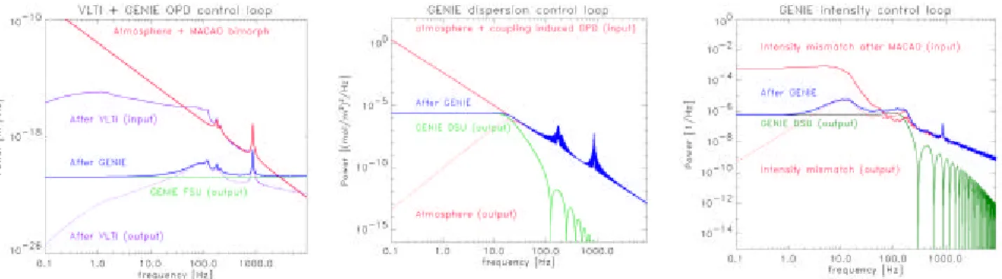
r

r

Figure 2. Illustration of the functioning of the control loops simulated in GENIEsim, by comparison of the power-spectral density

functions of the three main perturbations at the input and the output of the control loops.

star, the planet and the exo -zodiacal cloud, Ninstr, Nsky and Ndet are the signals due to respectively the IR emission, the

atmosphere and the dark current and read-out noise of the detector, and AM is the air mass between the telescopes and the target.

The ∆ϕi(t)and Pi(t) prohibit an evaluation of expression (1.) in closed form. In the code they are generated as random

realizations of power-spectral densities (PSDs). They originate in the atmosphere, which is assumed to have a Kolmogorov turbulence spectrum. In combination with Taylor’s hypothesis of a ‘frozen’ turbulence pattern blown in front of the telescopes by wind with a constant speed, this provides a prescription for the main atmospheric perturbations of the incoming wavefronts: piston9,10, longitudinal dispersion due to water-vapor,11,12 tip and tilt, Strehl ratio fluctuations, scintillation and fluctuations in the IR emission of the sky.13

In a first step, thes e perturbations are corrected by VLTI control systems: the VLTI OPD (optical path difference) controller, formed by the PRIMA FSU and the VLTI delay line, corrects the piston from typically 20 µm rms down to ~150 nm rms 14, the MACAO adaptive optics sytem corrects the tip, tilt and Strehl ratio fluctuations down to ~13 mas rms, and 6% rms resp.14 On the other hand, the VLTI environment adds not only to the IR background by 21 mirrors in between the target and GENIE, but introduces also some new perturbations. The bimorph mirror of the MACAO system adds ~30 nm rms of high-frequency piston, which is not corrected by the VLTI OPD control.15 The air in the delay line tunnels is turbulent and induces tip and tilt, of which the high-frequency part cannot corrected by the IRIS system, leaving an additional 9 mas rms of residual tip/tilt.14

Although these specifications are excellent for most of the interferometric applications, the requirements for nulling interferometry are rather more stringent. In particular the calibration requirements on the null, necessary for the detection of exo -zodiacal clouds at 10 to 20 times the Solar level, demand OPD control to a few nm rms. The GENIE OPD control loop therefore has to improve the VLTI piston residuals by another two orders of magnitude. This can be achieved with a high-frequency fringe-sensing unit (FSU).8 The GENIE dispersion control loop has to bring down the longitudinal dispersion by a similar amount, using an additional FSU, operating at another wavelength. In order to obtain sufficiently deep nulls it is necessary to clean the wavefront by injection of the light in to a single -mode waveguide (SMW, in our case a single mode fiber). The coupling efficiency with which the light can be injected into the SMW is influenced by tip and tilt. The intensity fluctuations, due to the residual Strehl fluctuations, and SMW coupling, have to be brought down to below 1% rms by an additional GENIE intensity control loop. Although injection of light into a SMW reduces all wavefront errors to intensity and phase fluctuations16 and the tip and tilt residuals coming from the VLTI are modest, there still may be a need for an additional tip/tilt control loop in GENIE.

Figure 3. Simulation of the detected total signal from τ Boo A + B at the output of the beam combiner. The signal is smoothed in order to demonstrate the small difference between the signal with and without the contribution from the planet.

Each of the above mentioned VLTI and GENIE control loop systems are modeled in GENIEsim, conform the illustration in Fig. 1. In Fig. 2, the operation of the three main GENIE control loops is shown. GENIEsim works mainly with PSDs to model the control loops, and only in the last stage random sequences of phase and intensity perturbations, based on the residual PSDs, are generated.

3. THE PROBLEM OF FLUX CALIBRATION

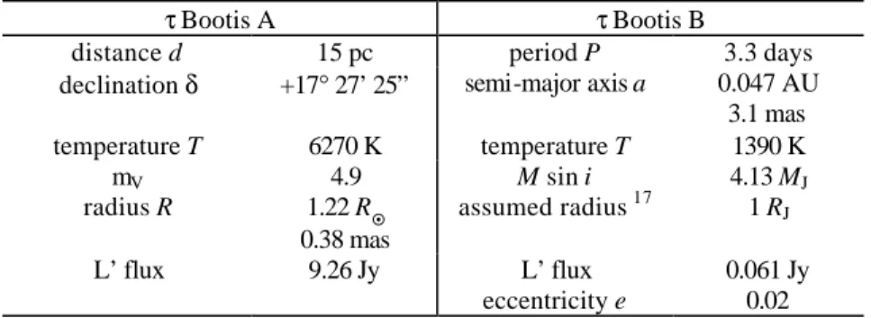
One of the more favourable planetary systems to observe with GENIE at the VLTI is τ Bootis A + B, whose properties are summarized in Table 1. It is relatively nearby, can be observed at a useful elevation from Paranal, the star is bright enough to allow the operation of the high-speed control loops, and the planet is in a close orbit, which ensures a high temperature, and therefore brightness of the planet, which gives in the L’ band a good match with the 89 m baseline between UT 2 and 4, and which allows rotational modulation of the planetary signal in a couple of nights.

Table 1. The main properties of τ Bootis A + B, an example of G-type star with a hot Jupiter companion.

τ Bootis A τ Bootis B

distance d 15 pc period P 3.3 days

declination δ +17° 27’ 25” semi-major axis a 0.047 AU 3.1 mas temperature T 6270 K temperature T 1390 K mV 4.9 M sin i 4.13 MJ radius R 1.22 R_¤ 0.38 mas assumed radius 17 1 RJ L’ flux 9.26 Jy L’ flux 0.061 Jy eccentricity e 0.02

Figure 4. The signal-to-noise ratio for the detection of the planetary signal and measurable null depth as a function of integration

time. The SNR improves over time approximately as t1/2_{. The measured null, defined as the ratio of the signal measured in the}

constructive output to that in the destructive output (including the planet) is limited by the stellar leakage, as the baseline had to be matched to the location of the planet. On similar stars nulls as deep as 1500 are achievable.1

Figure 3 shows the output of a simulated 1 hour observation of τ Boo with GENIE and two UTs under standard Paranal atmospheric conditions (1” seeing and a wind speed of 11 m/s). The top curve is the total detected signal, in photo-electrons, including leakage, planet and background. Below that, for illustration, exactly the same curve but without the planetary signal. The bottom curve shows the off-source signal, which is obtained in order to perform the background subtraction.

Figure 4 illustrates how the total signal-to-noise ratio of the planetary signal builds up during the exposure. Although the SNR reaches about 30 in one hour exposure, it is clear from a comparison of the two upper curves in Fig. 3 that it is near to impossible to establish whether the planet has been observed or not. As the period of τ Boo B is several days, the modulation of the planetary signal, consistent with the planet moving in and out of the fringe takes place over several hours and has to be observed over several consecutive nights. Over this period, the photometry has to be calibrated to a fraction of a percent, in fact, to a level below the fluctuations in the null. This is not only a tremendous challenge for the photometric calibration, but would require a considerable improvement of the GENIE performance as well.

4. OPD MODULATION

A practical solution to the problem of flux calibration is provided by the modulation of the optical path difference (OPD).7 The principle behind this technique is illustrated in Fig. 5. By modulating the optical path length in one arm of the interferometer, the transmission map is shifted in front of the objects in the sky. Such a modulation can be introduced quite simply as a sinusoidal offset to the zero point setting of the GENIE OPD controller. Starting from a situation where the valley of the transmission map (null) is centered on the star, any shift either to left or right will increase the stellar leakage. By placing the planet in between a crest and a valley (i.e. on the grey fringe), a shift of the transmission map to the right will decrease the planetary transmission while a shift to the left will increase it. This is achieved by selecting a smaller baseline (e.g. UT 3 and 4). As a result, the leakage is modulated at twice the frequency as the planetary signal, as in any other symmetric source such as the exo -zodiacal cloud. Hence both signals can be separated in frequency space. Fig. 6 demonstrates the application of this technique in practice, using a simulation of the equivalent of 1 hour of observation of τ Boo A+B with GENIE operated again under nominal VLTI conditions. For the sake of computational speed and memory, the actual computation was performed for a planet at the same temperature but with twice the radius of Jupiter. As this object will be 4 times as bright as nominal, the exposure time to be simulated was only 225 s, 1/16 of

an hour, in order to arrive at the same SNR. The modulation frequency was chosen well above the peaks in the residual PSDs for OPD, dispersion and intensity matching in Fig. 2, resulting in a low noise floor underneath the planetary peak in the spectrum. The modulation amplitude was 1 rad, sufficient to keep the planet on the ‘linear’ part of the fringe.7 Fig. 6a illustrates in an alternative way the necessity of a high enough modulation frequency. Here it is clear that the modulation is faster than the intensity fluctuations coming from residual phase and intensity perturbations.

Figure 6c indicates that the planetary peak extends some 400 standard deviations above the baseline. Unfortunately, it is not only the planetary signal that is modulated at the modulation frequency. If the null in the transmission map is not exactly centered on the star, e.g. due to a systematic offset, or quasi-static residuals in the OPD between the arms, that part of the stellar disk that is asymmetric with respect of the modulation of the transmission map will start to act as a pseudo-planet.

Figure 5. The principle of OPD modulation. By locating the planet on the steepest gradient of the transmission map (grey fringe), any

excursion of phase (OPD) induces a maximum change of the planetary signal, whereby in the illustrated case an increase of phase induces a decrease of planetary signal and vice versa. Provided the null in the transmission map is centered on the star, any phase excursion will only induce an increase in the stellar leakage. When the phase is modulated with a frequency fmod the stellar leakage is

therefore modulated at twice this frequency, allowing a separation of the planetary signal and the leakage in frequency space. The more modulation cycles are present in the data, the sharper the lines in frequency space will become.

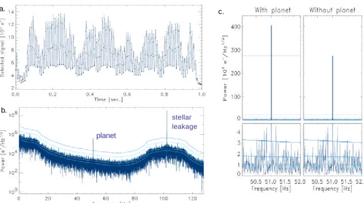
Figure 6a. One second of simulated output with OPD modulation in one arm. The modulation frequency is 51 Hz, which is faster

than (most of) the fluctuations in the signal due to variations in leakage and coupling. b. The Fourier transform of the full observation, clearly revealing the peak of the planetary signal, and the leakage at twice the modulation frequency. The solid lines indicate from bottom to top the location of, respectively, the local average (baseline) of the signal and 1, 3, 10 and 30 standard deviations above that average. c. Zoomed images of the planetary peak in Fig. 6b. Notice that the vertical scale is now linear. The top panels illustrate the difference in peak height with and without the planet, while the bottom panels show the noise level. Horizontal lines in the top panels indicate the 10 and 30 standard deviations above the baseline. Horizontal lines in the bottom panels indicate the locations of the average, 1 and 3 standard deviations above the average. The part of the peak above the dotted line is due to the planet, and will be modulated by the rotation of the Earth and the orbit of the planet around the parent star. The SNR of this modulation is ~170.

Even in the absence of a planet, there will seem to be a (pseudo-) planetary peak. Fortunately, the planet itself adds 50% to this peak. The difference with the pseudo-planetary signal is that the real signal is modulated due to Earth’s rotation and the motion of the planet around its parent. With this second source of modulation the planet can be detected with a SNR noise ratio of 170.

Figure 7 shows the source of the spurious planetary signal: the PSD of the total phase delay stays constant below 10 Hz, implying that there is an effective, quasi-stationary phase offset of ~0.5 mrad. Presently, the GENIE control loops are modeled in a rather simple way: by one or two consecutive PID stages. Since these are optimized to take a maximum amount of power from the fluctuation spectra, they act mainly at the higher frequencies. A more advanced design of the controller stages, using Kalman filtering or other techniques to minimize the power at the lowest frequencies, will reduce the quasi-stationary offset of the transmission map with respect to the center of the star, and thus the spurious planetary signal. Therefore, the SNR for the detection of the planet derived from Fig. 6c is likely to be on the conservative side.

stellar leakage planet

a. _c.

Figure 7. Power spectral density of the total phase delay in one arm of the interferometer at the entrance of the GENIE beam

combiner. The high-frequency peaks are a result of piston added by the MACAO bimorph mirror. This diagram shows the amount of residual power at low frequencies, responsible for the spurious planetary signal in Fig. 6b.

5. CONCLUSIONS AND OUTLOOK

Using numerical simulations of GENIE embedded in the VLTI environment, we have shown how OPD modulation provides a feasible solution for the problem of flux calibration, which hampers the detection of low-mass companions of stars with nulling-interferometric schemes. For a representative example, τ Boo A + B, it was demonstrated that within an hour a high enough signal-to-noise ratio could be obtained to allow the unambiguous detection of the planet. Evidently, this implies that brighter low-mass companions can be detected as well. The SNR is actually high enough to suggest the feasibility of warm Jupiter detection.

The SNR leaves enough room to divide the signal over several wavelength channels and perform low-resolution spectroscopy. This will not only allow a better distinction of the planet and spurious signals, but also opens the window to exo -planetary spectroscopy from the ground.

Because the planetary and leakage signal are separated in frequency by the OPD modulation, the requirements on the null depth, which only affect the strength of the leakage signal, and therefore the height of the leakage peak, are alleviated. In fact, suppression of low-frequency perturbations of the phase is now more important.

As the OPD modulation technique is sensitive to asymmetry in the source distribution on the sky with respect to the optical axis, it will not only pick up planets, but also spots on the stellar surface, or blobs in the exo -zodiacal cloud. At first glance this may seem a disadvantage from the perspective of planetary detection. However, radial velocity techniques suffer from star spots as well; in fact, all known hot Jupiters have been found around stars with very low levels of activity. From a broader astronomical perspective, this disadvantage may actually turn out to be an advantage which allows the observation of a broad range of phenomena which are presently outshone by strong nearby sources. It is evident that GENIE holds a large potential for astronomy extending beyond the realm of exo -planetary science.

ACKNOWLEDGMENTS

REFERENCES

1. P. Gondoin et al, “Darwin-GENIE: a nulling instrument at the VLTI”, Proc. SPIE 5491(2004)

2. P. Gondoin et al. “The Darwin Ground-based European Nulling Interferometry Experiment (GENIE)”, Proc. SPIE 4838, 700 (2003)

3. R. den Hartog et al., “Could GENIE detect hot Jupiters?”, in Proc. Towards Other Earths: DARWIN/TPF and the

Search for Extrasolar Terrestrial Planets, ESA SP-539, p. 399 (2003)

4. O. Absil et al., “Can GENIE Characterize Debris Disks Around Nearby Stars?”, in Proc. Towards Other Earths:

DARWIN/TPF and the Search for Extrasolar Terrestrial Planets, ESA SP-539, p. 317 (2003)

5. L.Kaltenegger et al., “Characterization of Disks Around YSO’s with GENIE”, in Proc. Towards Other Earths:

DARWIN/TPF and the Search for Extrasolar Terrestrial Planets, ESA SP-539, p. 465 (2003)

6. O. Absil, GENIEsim, the GENIE simulator, Diploma thesis, Université de Liège (2003)

7. L. d’Arcio et al., “Use of OPD modulation techniques in nulling interferometry”, Proc. SPIE 5491 (2004) 8. O. Absil et al., “Influence of atmospheric turbulence on the performance and design of GENIE”, Proc. SPIE 5491

(2004)

9. J.-M. Conan, G. Rousset and P.-Y. Madec, “Wave-front temporal spectra in high-resolution imaging through turbulence”, J. Opt. Soc. Am. A, Vol. 12, No. 7, 1559 (1995)

10. J.W. Goodman, Statistical Optics, John Wiley & Sons, 361 ff. (1985)

11. J. Meisner and R. le Poole, “Dispersion affecting the VLTI and 10 micron interferometry using MIDI”, Proc. SPIE 4838, 609 (2003).

12. C. Koresko et al., “Longitudinal Dispersion Control for the Keck Interferometer Nuller”, Proc. SPIE 4838, 625 (2003).

13. E. Bakker et al.,”Thermal background fluctuations at 10 micron measured with VLTI/MIDI”, Proc. SPIE 5491 (2004)

14. R. Wilhelm and P. Gitton, “The VLTI environment and GENIE”, in Proc. Towards Other Earths: DARWIN/TPF

and the Search for Extrasolar Terrestrial Planets, ESA SP-539, p. 659 (2003)

15. R. Arsenault et al., “MACAO-VLTI: An Adaptive Optics System for the ESO Interferometer”, Proc. SPIE 4839, 174 (2003)

16. C. Ruilier, Filtrage modal et recombinaison de grands telescopes. Contributions a l’instrument FLUOR, PhD thesis, University Paris VII (1999)