IAC-10-C2.2.6
THERMO-ELASTIC DISTORTION MEASUREMENTS BY HOLOGRAPHIC INTERFEROMETRY AND CORRELATION WITH FINITE ELEMENT MODELS FOR SIC CONNECTIONS/JUNCTIONS
ON SPACECRAFT
F. Eliot
ASTRIUM, France, [email protected],
C. Thizy CSL, Belgium, [email protected], A. Shannon ESTEC, The Netherlands,
[email protected], Y. Stockman CSL, Belgium, [email protected], D. Logut ASTRIUM, France, [email protected]
The objective of this study is to improve and develop analytical connections modelling guidelines that can have a preponderant impact on instruments stability.
For that purpose, samples have been designed to be representative of glued and bolted connections/junctions that can be encountered in stable structures on spacecraft. In this study, material characteristics are assumed to be
well known: Silicon Carbide (SiC) and Titanium (TA6V) have been retained.
For the tests, temperature variations between -20K and +15K from ambient have been applied to the samples. Thermo-elastic distortions have been measured with a holographic camera. This holographic camera can measure displacements in the range of 20 nm to 20 µm without physical contact with the samples.
The tests results have been compared to the predictions obtained by Finite Element Modelling. From this comparison modelling guidelines have been issued with the aim of improving the accuracy of computed thermo elastic distortions.
A second phase to this study is planned. The objective is to implement all the benefits on improvement of thermo-elastic distortions predictions and verification achieved during the first phase on real spacecraft hardware.
I. INTRODUCTION
Scientific, earth observation and telecommunication spacecrafts are submitted to severe thermal environments while their mission performance requires more and more high stable structures. Due to on-ground constraints, the verification by test of the performances of these stable structures is usually limited. Therefore accurate prediction methodology and verification capability of thermal distortions becomes mandatory for ensuring the in-orbit performance objectives of future programs.
The main thermo-elastic contributors of the final stability performances are the material and assembly physical properties knowledge (Coefficient of Thermal Expansion, Young
modulus, Poisson ratio…), the modelling and simulation capabilities (temperature mapping, accurate thermo-elastic finite element models) and the verification test performances. Advanced measurement techniques are required to characterize and determine the different main contributors to the final end to end performance and to perform accurate correlation.
In this study, material characteristics are
assumed to be well known: SiC/SiC and SiC/TA6V glued and bolted samples have been retained.. The objective of this study is to improve and develop analytical connections modelling guidelines by
II. SAMPLES DESCRIPTION
The samples have been defined based on the following criteria.
They have to be representative of bolted and glued connections that we can encounter in the vicinity of sensitive areas.
Their design has to be simple as the correlation focus is on junctions modelling rather than assembled parts themselves.
The samples materials are currently encountered in stable structure and their physical properties well-known: Silicon Carbine (SiC), Titanium (TA6V), EA9321 glue, stainless steel bolts and washers have been retained.
The size of the samples and their distortions amplitude answer to CSL measurement and test devices constraint: holographic Camera, 20nm to 20µm displacements, in a 500mm diameter vacuum chamber.
Finally, the samples have to show positive margins of safety when submitted to interface planarity defaults (bolted samples) and thermal loads.
Eight samples have been identified: two locally glued samples (SiC/SiC and SiC/TA6V), four globally glue samples (2 SiC/SiC and 2 SiC/TA6V with 0.1 or 0.3 mm joint of glue), two bolted samples (SiC/SiC and SiC/TA6V). The samples
Fig. 1: Globally glued samples geometry
Fig. 2: Locally glued samples geometry
Fig. 3: Bolted samples geometry
II. TESTING DESCRIPTION AND RESULTS II.1 Holographic camera technique
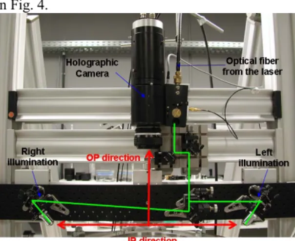
The holographic camera (HC) developed by CSL [1], [2] has been used to measure the thermo-elastic distortions. It is composed of a compact optical head and an electronic rack containing the 5W Nd-YAG laser operating at 532 nm. An optical fibre brings the light from the laser to the optical head, which makes it a flexible instrument. Relative displacements ranging from 20 nm to 20 µm can be
contactless. A first step consists in recording the hologram of the object under test, the reference state. Then, a stimulation (thermal or mechanical) is applied to the object. Finally the hologram is readout; the interference pattern resulting from the superposition of the wave front diffracted by the hologram (reference state of the object) and the one coming directly from the object (deformed state of the object) is recorded on a CCD camera. The phase image obtained is composed of a fringe pattern representing the relative displacement of the surface. This phase image is then unwrapped to obtain the continuous relative displacement. A unique feature of this holographic camera is that it uses a photorefractive crystal (PRC) as the recording medium, which allows in-situ recording and erasure of the hologram. Each hologram readout partially erases the hologram, which means that only typically 4 readouts can be performed from the same recording. Nevertheless, successive measurement sequences (hologram recording and readout) can be performed indefinitely, which allows measuring large displacements. The relative displacements are measured out-of-plane because of the object illumination and observation geometry. However, for this study, a two-illuminations configuration has been implemented [3], as shown in Fig. 4.
Fig. 4: two-illuminations configuration of the HC Two holograms are simultaneously recorded in the PRC, the readout is sequential. In this configuration, the relative out-of-plane and in-plane (in one direction) displacements are measured. The uncertainty for both measurements is 40 nm. In this configuration only two acquisitions can be performed from the same reference, compared to the four with one illumination. To obtain the correct relative displacements, one has to know the absolute in-plane or out-of-plane displacement of one point in the field of view of the HC, or the relative in-plane or out-of-plane displacement between two points. A scaling is then applied to the data. For this study this additional processing is possible since the CTE of SiC is well known. The SiC : 120 mm diameter and 5 mm thick
SiC or TA6V :
75 mm diameter and 5 mm thick
0.2 mm joint of glue EA9321: M6 Stainless steel screws SiC or TA6V: 75mm diameter 5 mm thick
SiC : 120 mm diameter and 5 mm thick.
SiC : 120 mm diameter 5 mm thick for SiC/SiC and 9 mm for SiC/TA6V samples
SiC or TA6V:
75 mm diameter and 5 mm thick for SiC samples and 3 mm thick for TA6V
EA9321 glue: 0.1mm or 0.3mm thick sample
II.2 Test facility
The samples are located in a vacuum chamber with an inner diameter of 500 mm and a height of 545 mm. The primary pump used allows reaching a vacuum of about 10-2 mbar. The SiC samples lie on an Invar bench mounted on three Invar blades screwed to the bottom flange of the chamber. The temperature variations of the samples are obtained by circulating, with a chiller, a mix of glycol and water in a shroud located underneath the Invar bench. The temperature range achievable with this chiller is from - 28°C to 60°C. Thermocouples are available in the chamber to monitor the temperature on the samples. The support of the HC is an assembly of columns to make it as stable and rigid as possible. The whole set-up is placed on an optical table (Fig. 5).
Fig. 5: Test set-up II.3 Testing
Two test campaigns have been performed: one for the four SiC/SiC samples and one for the four SiC/TA6V samples.
II.3.1 SiC/SiC samples
Fig. 6: Integration of the SiC/SiC samples in the vacuum chamber
Fig. 6 shows the samples arrangement in the vacuum chamber. Each sample was equipped with four thermocouples, two on the large disc and two on the small disc. These were glued on the side of the discs to reduce the noisy areas in the results due to the stickers. The samples have been coated with white powder to improve the diffuse reflection of the laser light.
The success criteria of the test were defined as follows:
• Homogeneous temperature on samples achieved for each acquisition: less than 0.5 K variations in the sample (in plane and in the height of the sample).
• Comparison with reference case after heating or cool down shows no samples variations.
• Shape of the computed displacements is comparable with the predictions. The displacements measured, Peak-to-valley (PTV), discrepancies with the predictions are within +/-25%.
The test sequence is described in Fig.7. The criterion for the temperature stabilisation was to have less than 0.1°C variation over 10 minutes for each thermocouple.
An example of phase images obtained with the HC is presented in Fig. 8. The post processing of the results consisted in scaling the data for each sample by using the SiC CTE. This was possible for these SiC/SiC samples since bi-metallic effects were negligible.
Also, the tilts in the out-of-plane relative displacement results, caused by the rigid body movements of the samples, were removed by computing the Zernike coefficients. An example of out-of-plane and in-plane displacements measured on the bolted sample is presented in Fig. 9. The noisy areas are due to the screws, the stickers of the thermocouples and the shadow of the small disc on the large one that prevents the unwrapping algorithm from performing well in these areas. The success criteria have been matched for all the samples.
Fig. 7: SiC/SiC samples test sequence
Fig. 8: Phase images for the SiC/SiC samples, cold case RT-10°C
Fig. 9: Out-of-plane (left) and in-plane (right) displacements of the bolted SiC/SiC sample for the cold case RT-10°C
II.3.2 SiC/TA6V samples
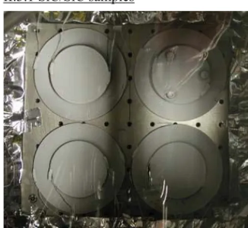
Fig. 10 shows the samples arrangement in the vacuum chamber. Each sample was equipped with two thermocouples, one on the large disc and one on the small disc, glued on the face of the discs to avoid ungluing. The samples have been coated with white powder to improve the diffuse reflection of the laser light.
Fig. 10: Integration of the SiC/TA6V samples in the vacuum chamber
The success criteria were the same as for the previous test. The test sequence is described in Fig. 11. An example of phase image obtained with the HC is presented in Fig. 12.
Fig. 11: SiC/TA6V samples test sequence
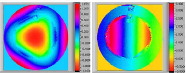
In this test, the material of the small and large discs was different, the bi-metallic effect therefore did not allow the scaling of the results for each sample by using the SiC CTE. To overcome this problem, a reference SiC disc was implemented between the four samples (as shown in Fig. 10). For this solution to work correctly, the samples had to be in contact with the reference disc to have continuity between the samples and the reference disc, in order to link the displacement of the reference disc to the displacement of the samples. The tilts in the out-of-plane relative displacement results were removed by computing the Zernike coefficients. An example of out-of-plane and in-plane displacements measured on the locally glued sample is presented in Fig. 13. The noisy areas are due the stickers of the thermocouples and the shadow of the small disc on the large one that prevents the unwrapping algorithm from performing well in these areas. The success criteria have been matched for all the samples.
Fig. 12: Phase images for the SiC/TA6V samples, cold case RT-5°C
Fig. 13: Out-of-plane (left) and in-plane (right) displacements of the locally glued SiC/TA6V sample for the cold case RT-5°C
III. FINITE ELEMENT MODELS DESCRIPTION
Nastran 2006 software has been used for modelling and thermal distortions computation.
III.1 Glued samples
Two detailed Finite Element Models (FEM) models have been built: an unstructured FEM, using quadratic CTETRA elements and a structured FEM, using CHEXA and CPENTA elements. The structured FEM has been used for number of elements in thickness sensitivity. A view of those FEM is provided Fig.14.
Unstructured Mesh Structured Mesh Fig. 14: Globally glued FEMs
The joint of glue is modelled either with 3D elements or with zero-length elastic elements (representative of glue stiffness).
Iso-static boundary conditions are applied. The glue thickness impact is also studied: samples with 0.1 and 0.3 mm joint of glue are tested and compared to the FEM.
III.2 Bolted samples
As for the glued samples, two modelling assumptions have been studied for the discs: an unstructured FEM using quadratic CTETRA elements and a structured one using CHEXA and CPENTA elements have been built.
The FEM allows predicting the impact of bolt preload variation with temperature on thermal distortions: the free part of the bolt is modelled by beams elements.
The impact of the washer on the thermal distortions is also studied: the washer is modelled using three dimension elements. A view of the bolted FEM is provided in Fig 15. The washers are represented in green.
Structured Mesh
Unstructured Mesh Fig. 15: Bolted samples FEM
Different disc-washer and bolt-washer interface modelling were tested such as:
• Having a “perfect” (i.e. “merged”) or a purely “sliding” disc-washer interface
•
Modelling the bolt-washer interface with either RBE3 or expandable RBE2 spiders in light blue in Fig. 15.Models without explicit modelling of the washer have also been tested: bolts are directly connected to the disc with bars, RBE3 or expandable RBE2 spiders on an area representative of the washer footprint.
IV.CORRELATION PROCEDURE IV.1 Procedure description
Each time, In-Plane (IP) (along X axis) and Out-of-Plane (OP) displacements are computed and compared to tests results.
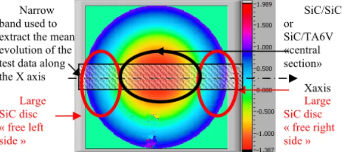
To allow a direct comparison between the Finite Element Model results and the test, we have chosen to plot the displacements along X axis on the samples (that is why the FEM have been built with a line of nodes along X axis). Fig. 16 shows area for which measured displacements have been posprocessed.
Fig. 16: Area used for test/prediction comparison It is important to underline that the HC provides relative displacements. If a jump higher than half the HC wavelength (266 nm) occurs between two consecutive pixels, the test data have to be corrected of n*266nm (n to be computed with the help of FEM predictions): see V.1.1.
During heating and cooling down, an intermediate step of temperature has been made to help in total delta T distortions understanding.
Quantitative data are extracted from FEM prediction by (linear) polynomial fitting and compared with the test data ones.
IV.2 SiC/SiC samples
The temperature variations applied around room temperature are +15°C for the “Hot Case” and -20°C for the “Cold case”.
Globally glued samples are used for joint of glue modelling guidelines: the two SiC discs have the same thickness.
Locally glued sample is used to check if modelling guidelines issued for joint of glue allow to reach a good correlation.
Bolted samples are used to issue modelling guidelines for preload variation and washer impact on thermal distortions.
IV.3. SiC/TA6V glued samples
The temperature variations applied around room temperature are +5°C for the “Hot Case” and -5°C for the “Cold case”.
Those samples are used to predict the bending due to “bi-metallic» effect.
Globally glued ones have allowed issuing modelling guidelines for SiC and TA6V discs.
Locally glued samples are used to confirm the guidelines issued for glue and discs modelling.
Bolted samples are used to confirm guidelines issued from SiC/SiC bolted samples for interface modelling and allows to issue guidelines for discs modelling.
V. CORRELATION RESULTS V.1. SiC/SiC globally glued samples
V.1.1. Out of Plane data correction / poisson coefficient impact
As described in the correlation procedure, half wavelength “jumps” are to be corrected on OP tests results. The displacements “step” between the small and large disc is mainly due to the joint of glue contraction/expansion with temperature variations.
Analytical estimation of the number of jumps “j” between small and large discs:
e= thickness
α= Coefficient of Thermal Expansion ∆T= Temperature variation.
of measured OP displacements.
Fig. 17: SiC/SiC globally glued OP displacements correction
An analytical estimation of the number of half-wavelength jumps to be corrected does not allow matching the FEM results except if the glue poisson ratio is set to zero: one dimension analytical evaluation ignores its impact. The impact of poisson ratio of the glue on the OP (“piston” like) displacements is to be assessed using the Finite Element Model (FEM).
Taking the poisson ratio of the glue into account in the FEM, leads to a corrective jump of 4x266 nm instead of the 2x266 nm computed the analytical evaluation. Applying this 4*266 nm correction on test OP displacements, allows to reach a good correlation between FEM and test.
Large SiC disc « free left side » Large SiC disc « free right side » SiC/SiC or SiC/TA6V «central section» Xaxis Narrow band used to extract the mean evolution of the test data along the X axis
T
e
e
j
th=
(
glue⋅
α
glue+
disc⋅
α
disc)
⋅
∆
2 43 . 2 266 648 648 ⇒− ≈− ⇒ − ≈ nm nm nm jth Jumps correction
V.1.2. Impact of joint of glue modelling 3D joint of glue modelling
The element type (Hexa or Tetraparabollic elements) and the number of elements in the joint of glue thickness impact on computed OP distortions is provided on Fig. 18. And 19.
Fig. 18: OP free part of large disc cold case
Fig. 19: OP free part of large disc cold case The glue contraction impact on thermal distortions is slightly underestimated whatever the modelling assumptions are.
Hexa elements give better results than tetraparabollic ones.
One element in the joint of glue thickness is sufficient (variations lower than 3%).
The impact of joint of glue modelling is negligible on In Plane (IP) displacements.
Elastic elements joint of glue modelling
The joint of glue is modelled by zero length elastic elements representative of the joint of glue stiffness: this modelling does not allow simulating the impact of the joint of glue contraction due to cool down. FEM/Tests results comparisons are provided on Fig. 20 and 21.
Fig. 20: OP cold case
Fig. 21: IP cold case
The computed OP displacements of the small disc only take into account the small disc contraction.
The computed OP displacements of the large disc free parts are only the contraction of the large disc and no more bending is observed: this confirms that the bending observed of the free part of the large disc is due to glue contraction.
Using elastic elements for joint of glue modelling has no impact on IP displacements. IP displacements are well predicted whatever the glue modelling assumptions are (within the measurement tolerances).
V.1.3 SiC/SiC globally glued samples correlations conclusions
The OP displacements half wave length jumps correction need the use of the FEM with 3D modelling of the joint of glue.
The OP displacements on the small disc are well predicted providing that a 3D modelling of the joint of glue is used: between -7 and -14% versus tests results.
The slope of the free part of the large SiC disc is due to glue contraction/expansion: it is predicted only with a 3D modelling of the joint of glue. This slope is underestimated but remains inside the HC uncertainty area. The best correlation is obtained for Hexa modelling with only one element in the joint of glue thickness and real samples thicknesses: -37.31% versus measurements. The glue effect is underestimated.
IP displacements are well predicted due to the SiC CTE hypothesis and the impact of the modelling assumptions negligible.
V.2. SIC/TA6V globally glued samples V.2.1. Tests results
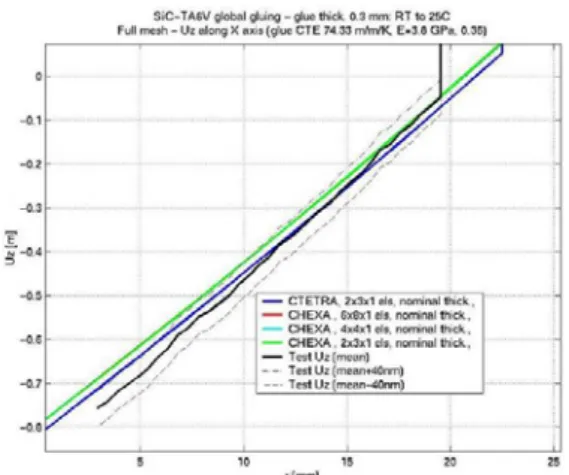
OP and IP measured displacements are compared with the FEMs simulation on Fig. 22 and 23:
Fig. 22: Tests OP: 0.3 mm joint of glue
Fig. 23: Tests IP: 0.3 mm joint of glue
On OP displacements, we can observe the bending of the sample due to “bi-metallic” effect.
On IP displacements, we can notice an increase of slope on TA6V/SiC bonded area which corresponds
to a 6.37E-6 m/m/K CTE (higher than CTE found using mixing rule: 2.9E-6m/M/K as the measure is made on the top of the TA6V disc).
V.2.2. Impact of discs modelling
The impact of elements type (Hexa or tetrapabollic) as well as the number of elements in the thickness of the discs is provided on Fig. 24 and 25.
Fig. 24: Tests/FEM OP: 0.3 mm joint of glue
Fig. 25: Tests/FEM IP: 0.3 mm joint of glue HEXA elements are to be used rather than Tetraparabollic ones: they allow achieving a better correlation of OP displacements.
Two elements in discs thickness is enough to reach a good prediction of the bending effect. Increasing the number of elements in the thickness has a negligible impact on the predictions.
IP displacements are well predicted whatever the modelling assumptions are for the discs.
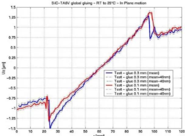
V.2.3. Impact of glue thickness on IP displacements
Two globally glued SiC/TA6V samples are studied: one has a 0.1 mm joint of glue and the other one a 0.3mm joint of glue. The impact of the joint of glue thickness on the measured IP displacements is provided in Fig. 26.
Fig. 26: Glue thickness impact on IP displacements
The slope over the TA6V disc of the 0.1 mm glue sample is lower than the 0.3 mm glue sample. The CTE of the glue is thus dominant on its Young modulus. A similar behaviour was found with FEM modelling.
To be conservative, it is recommended to model the joint of glue with its maximal thickness that is including its manufacturing tolerance.
V.2.4. SiC/TA6V globally glued samples correlations conclusions
Maximum deflexion is well predicted providing that three dimensions (3D) elements are used for the glue: between -1.1 and 2.4%. Hexa elements give the best correlation and two elements in the discs thickness are sufficient.
The slope of the SiC free side is underestimated by 8% but remains within the test tolerances. This improves by increasing the glue stiffness.
IP displacements are well predicted on the large disc free side: delta +2% versus the test.
IP displacements at the TA6V disc level are underestimated (-16% versus the measured displacements). A temperature gradient has been measured on this sample (∆T=5.1°C over the TA6V disc and ∆T=4.7°C over the SiC disc). Considering this gradient in the simulation, the underestimation is reduced to -8%.
V.3. SiC/SiC Locally glued samples
Modelling guidelines issued from global gluing correlation are applied to locally glued FEMS: • Structured finite element mesh with CHEXA and
CPENTA elements;
• A single 3D element within the joint of glue thickness;
• More than 2 elements in discs thickness (4 elements in the large and small disc thickness).
1.1.1.1. 1.1.1.2. 1.1.1.3. 1.1.1.4.
Fig. 27:Tests/Predictions: OP Cold case
1.1.1.5.
Fig. 28: Tests/Predictions IP Cold case The OP deflexion is overestimated by +3.2% for the hot case and underestimated by -2.2% for the cold case.
IP displacements over the small disc are overestimated by +8.5% for the hot case and by +2.6% for cold case.
A good correlation of the predictions versus tests is found: this confirms the modelling guidelines issued from globally glued samples study.
V.4. SiC/TA6V Locally glued samples
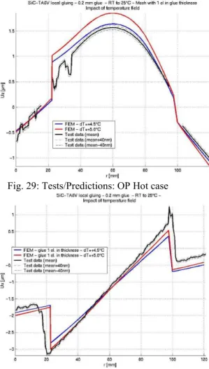
As for SiC/SiC samples, modelling guidelines issued from global gluing correlation are applied. Results are provided on Fig. 29 and 30.
Fig. 29: Tests/Predictions: OP Hot case
Fig. 30: Tests/Predictions: IP Hot case The discrepancy in terms of overall OP deflexion is less than 5%.
The slope of the IP displacement over the small TA6V disc is underestimated by about 7%.
A good correlation of the predictions versus test is found: this confirms the modelling guidelines issued from globally glued samples study.
V.5. SiC/SiC Bolted samples V.5.1. Correlation processing
The measured displacement fields are highly disturbed around the washers and bolts’ heads and nuts: it is impossible to correct OP displacements amplitude.
Therefore, the comparison of the predictions and tests has been split into three areas (Cf Fig. 30) defined as follows:
The maximal amplitude of OP deflection between the centre C of the upper surface of the small disc and grid point A located on its outer diameter is analysed
The slope of the OP displacements curves, over the large disc free SiC side, (left and right side) are analysed.
Fig. 31: Tests/Predictions correlation areas The left, centre, and right sections of the test and prediction curves were shifted independently and appropriately so that they have the same mean value over each section.
Any information about the relative position of the prediction curves with respect to the test data is lost: only the comparison on their shape is here meaningful.
V.5.2. Washer modelling impact
The washer modelling impact on thermal distortions is provided in the chapter.
Washer 3D modelling
Fig. 32: Tests/Predictions: OP Cold case
The Green curve concerns 3D stainless-steel washers merged with the disc: OP displacements are overestimated.
The Light blue curve concerns a 3D stainless-steel washers model which interface with the disc is perfectly sliding FEM. It correlates quite well OP displacements. Sliding of the washer occurred during cooling down tests (MoS2 lubricated washer: friction coefficient about 0.1).
X A
The washer contraction impact on the OP distortions is significant: the washer has to be modelled.
Fig. 33: Tests/Predictions: IP Cold case
The impact of the washer on the IP distortions is not significant: a good correlation is achieved whatever the washer modelling assumptions are.
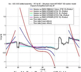
Washer simplified modelling
Fig. 34: Tests/Predictions: OP Cold case The Red curve concerns the washer modelled by an expandable RBE2 (washer CTE) which overestimates OP results by more than 200%.
The Blue curve concerns the washer modelled by beams (diameter=washer thickness and CTE=washer one). This highly overestimates OP displacements.
The light blue curve concerns the Washer modelled by an expandable RBE2 (SiC CTE). This highly underestimates OP displacements.
The Pink curve concerns the washer modelled by RBE3 elements. This modelling improves the prediction but OP distortions are underestimated.
V.5.3.Connection between bolt and washer modelling impact
Expandable RBE2, RBE3 elements have been used to connect the bolt (modelled by 1D beam elements) to the washer (3D modelling).
The simulations comparison with the tests measured OP displacements are provided on Fig. 35 (Cold Case).
Fig. 35: Tests/Predictions: OP Cold case
The Light blue and red curves concern merged washer and expandable RBE2 connection between bolt and washer: this leads to OP displacements highly overestimated.
The Pink curve concerns sliding washer and RBE3 bolt/washer connection: OP displacements are underestimated.
The Green curve concerns expandable RBE2 bolt/washer connections: OP displacements are underestimated.
The Blue curve concerns washer+RBE3 connection between the bolt and washer. This is the best solution to be on the conservative side.
V.6 SiC/TA6V Bolted samples V.6.1. Correlation processing
The correlation processing is identical to the one used for the SiC/SiC bolted sample in paragraph V.5.1.
V.6.2. Disc/Disc and Disc/Washer interface modelling impact
Merged meshing between discs and discs washer are compared to perfect sliding modelling between the two discs or between the washers and the small disc: See Fig. 36 and 37 for OP and IP simulations to tests results.
Fig. 36: Tests/Predictions: OP Cold case
Fig. 37: Tests/Predictions: IP Cold case
The Red curve concerns sliding disc-washer I/F and merged disc-disc I/F: OP displacements are overestimated.
The Pink curve concerns sliding disc-washer I/F and sliding disc-disc I/F: OP displacements are underestimated.
The Green curve concerns merged disc-washer I/F and sliding disc-disc I/F: OP displacements are underestimated.
The Blue curve concerns merged disc-washer I/F and merged disc-disc I/F: OP displacements are well correlated. This is the modelling assumptions to retain.
VII. MODELLING GUIDELINES VII.1: In Plane Gluing
These modelling guidelines results in good correlation with regards to tests measurements in the frame of:
In-plane distortions (parallel to joint of glue); Out-of-plane distortions (perpendicular to joint of glue).
Fig. 38: Illustration of “in plane” gluing Part 1 and 2 modelling:
3D model with structured mesh, CHEXA or CPENTA, with a minimum of two elements in each part thickness are to be used. This type of mesh allows to capture the bending behaviour (especially if part 1 and part 2 have not the same thickness or are not in the same material: bi-metallic effect) and opens the possibility to have axi-symmetric meshes.
Glue modelling:
Those recommendations are issued mainly from the out of plane correlations as the in-plane ones are not significantly impacted by the joint of glue modelling assumptions.
The joint of glue have to be modelled using 3D structured CHEXA or CPENTA element (obtained by surface extrusion for instance).
One element in the joint of glue thickness is sufficient.
It is recommended to model the joint of glue at it maximum thickness pending of the gluing tolerances (conservative approach). When the joint of glue is thicker, it is more flexible but the volume expanded with temperature variations increases and this phenomenon is dominant.
The variation of Young modulus, CTE and poisson ratio of the glue with the temperature are to be taken into account: average values between initial and final temperature must be used.
Part 2 Part 1 Joint of glue
V.II. Bolted Interface
The aim of these modelling guidelines is to model the impact of:
• the bolt preload variation with the temperature (no athermalisation washers).
• The washers expansion/contraction with temperature variations.
• part 1 and part 2 bimetallic effect in case of different material for part 1 and part 2.
Fig. 39: Illustration of “Bolted I/F” Part 1 and part 2 modelling:
A 3D model with structured CHEXA or CPENTA mesh, with a minimum of two elements in the thickness has to be used because this type of mesh allows capturing the bending behaviour (especially if part 1 and part 2 have not the same thickness or are not in the same material: bi-metallic effect).
A “merged” interface between part 1 and part 2 has to be considered.
Bolted interface modelling:
An explicit 3D (CHEXA or CPENTA) model has to be used for the washer.
A “merged” interface between the washer and the Part 1 and Part 2 has to be considered to be on the conservative side (no washer sliding).
To have the impact of the bolt contraction or expansion with the temperature on the thermal distortions, it is necessary to represent the bolt by beam elements using the bolt section and material properties to have the expected preload variation with the temperature. The axial force due to thermal load in the beam can be computed and compared to the analytically computed preload variation. The beam for bolt modelling begins bellows the screw head and ends at nut level (beam to be connected to the external parts of the washers). For bolt/3D washer interface, RBE3 elements have to be used on the screw head or nut footprint area.
Fig. 40 “Bolted Interface” modelling VIII. CONCLUSIONS VII.1. About tests data
Two illuminations test and a reference allow computing OP and IP displacements along one axis.
A SiC disc has been used for SiC samples (SiC CTE is an input data corroborated by tests).
The provided raw data being relative displacements, modifying them to get absolute displacements data was not straightforward. The correct evaluation of the “half-wavelength jumps” is not always easy even for such “simple” structure due to the impact of the glue material property, in particular its Poisson ratio.
As a consequence, if future correlations are to be made on more complex structure assemblies, in particular for phase 2 of this study, the use of several illuminations to get a full 3D displacements field might be necessary.
In order to reduce noisy areas and therefore the loss of data on the tested objects, the number of TMCs in the field of view of the HC can be reduced in combination with the use of a thermographic camera.
VII.2 About correlation results
FEM predictions leads to quite good correlations with the test data in both the out of plane and in-plane responses, if the correct joint of glue thickness, applied temperature field and interface modelling are taken into account in the model.
Modelling guidelines proposed both for joint of glue and bolted interface representations allow to reach a correlation with measured displacements on the samples better than 10% or within the test tolerances.
Washer
Part 2 Part 1
Washer
Nut (dark grey) Screw (light grey)
washers
bolt
RBE3
Part 1
A correct interface modelling is mandatory to capture the correct test behavior: this was particularly the case for the SiC-SiC bolted assembly, where the presence of disc-washer sliding was put into lights by the FEM predictions, which was afterward corroborated by a precise inspection of the test procedure (lubricated washer used).
REFERENCES
[1] M.P. Georges, V.S. Scauflaire, P.C. Lemaire, "Compact and portable holographic camera using photorefractive crystals. Application in various metrological problems", Appl. Phys. B 72, 761 (2001).
[2] M. Georges, C. Thizy, V. Scauflaire, S. Ryhon, G. Pauliat, P. Lemaire, G. Roosen, "Holographic interferometry with photorefractive crystals : review of applications and advances techniques", Speckle Metrology 2003, SPIE Vol. 4933, pp. 250-255, Trondheim, Norway, 2003.
[3] C. Thizy, M. Georges, V. Scauflaire, P. Lemaire, S. Ryhon, "In-plane and out-of-plane holographic interferometry with multibeam photorefractive recordings in sillenite photorefractive crystals", Trends in Optics and Photonics Series, Vol 87 on Photorefractive Effects, Materials and Devices, A.A. Sawchuk, ed., p. 504-510, La colle-sur-Loup, France, June 2003.