Testing a Mixture Model of Single-Peaked
Preferences
Smeulders, B.
∗ AbstractSingle-Peaked preferences play an important role in the social choice literature. In this paper, we look at necessary and sufficient conditions for aggregated choices to be consistent with a mixture model of single-peaked preferences for a given ordering of the alternatives. These conditions can be tested in time polynomial in the number of choice alternatives. In addition, algorithms are provided which identify the underlying ordering of choice alterna-tives if the ordering is unknown. These algorithms also run in polynomial time, providing an efficient test for the mixture model of single-peaked preferences.
1
Introduction
Preferences play an important role in many areas of research. When faced with different alterna-tives, be it different cars, candidates in an election, budgets, etc., it is commonly assumed that people have a preference ordering over all of these alternatives, ranking them from best to worst. Often the nature of the alternatives restricts the possible preferences. An important restriction is given by single-peakedness, introduced by Black [3]. Suppose a linear ordering exists, which ranks all alternatives along a line. An agent’s preferences are then single-peaked if she has a most preferred alternative, the peak, and when comparing two alternatives that are both on the same side of the peak, the alternative closest to the peak is preferred. This restriction is very natural when considering a situation where a single attribute of the alternatives drives the choice, for example, an election where candidates range from left to right wing or choices over budgets of various sizes. Given these examples, it is no wonder that this restriction has gained central importance in the areas of political science and social choice. Apart from being an appealing model in these areas, the assumption of single-peaked preferences has led to interesting theoreti-cal results. For example, aggregation of single-peaked preferences avoids the Condorcet paradox [3].
Given the importance of single-peaked preferences, it is of interest to test if and in which situations agents hold such preferences. A number of algorithmic papers have appeared on the subject. Given the complete preference profile of agents Bartholdi and Trick [2] provide a poly-nomial time algorithm to test whether these are single-peaked with respect to some ordering of the alternatives and to identify this ordering. Doignon and Falmagne [10] provides a different algorithm for this problem with a better worst-case bound. Escoffier et al. [15] rediscovered this algorithm and give a detailed description. Ballester and Haeringer [1] give two forbidden sub-structures, whose absence is a necessary and sufficient condition for the given preference profile to be consistent with peakedness. Puppe [26] gives a global characterization of the single-peaked domain. Furthermore, Trick [33] provides an algorithm for recognizing single-single-peakedness on trees, which again runs in polynomial time. Doignon and Falmagne [10], Knoblauch [19] and Elkind and Falizewski [13] investigate a closely related preference restriction, one-dimensional Euclidean preference profiles, and all provide polynomial time algorithms. Preference profiles
∗QuantOM, HEC Management School, Universit´e de Li`ege. The author is a post-doctoral fellow of the
that are nearly-single peaked are investigated by Erd´elyi et al.[14] and Bredereck et al.[6]. Test-ing for sTest-ingle-peakedness given real-world preference orderTest-ings is done by List et al. [20] and Sui et al.[32].
One common factor in these papers is that they test for single-peakedness given full preference profiles of the agents. However, there are several drawbacks to using this kind of data. First, it assumes that choices are made based on preference orderings. Agents who use a different decision rule, for example heuristics, can not accurately report their decision rule. Second, even if the assumption of preference orders is correct, there is a high risk that the ordering is misreported. This can be due to a simple error, as ranking all alternatives is a complex task, or because the agent has little incentive to determine her ranking over average alternatives.
The dominant setting for experiments in choice behaviour research is two-alternative forced choice (see Luce [21], Block and Marschak [4]). In this setting, agents are faced with choices between two alternatives, and must choose one. A large number of such choices are given, in-cluding repetitions of the same choice situations. This simple choice situation reduces the risk of agents misreporting. In the simplest situation, agents will consistently make the same choice when faced with repetitions of choice situations. However, it is very common that agents exhibit choice reversals. The data resulting from such experiments is thus, for every pair of alternatives, a rate with which one alternative is chosen over another. In this paper, it is our goal to provide a way of testing for single-peakedness in this setting, continuing a line of research started by Dridi [12].
To test for single-peaked preferences, while being able to account for choice reversals, we will make use of a ‘random preference model’ or ‘mixture model’, which can be traced back to Block and Marschak [4]. Such a model considers all possible ways a ‘core theory’, here single-peaked preferences, can be satisfied. It states that at any given point in time, the agent has a single-peaked preference, but that these may be different single-single-peaked preferences at different points in time. The data is consistent with this model if there exist single-peaked preferences, and a probability distribution over these preferences, such that the probability that the agent holds a preference in which she prefers one alternative over another is equal to the rate at which she chooses that alternative over the other. Notice that this model may also be used on the level of a population. The rate at which a population chooses one alternative over another can be determined by polling. The probability function then represents the probability that a member of the population holds a particular preference. The conditions such mixture models impose on data have been studied for a number of different classes of decision rules. It should be noted that aggregation of preferences in this way may lead to artifacts complicating analysis of the data (Davis-Stober et al.[9]). There is an equivalence between testing mixture models and the membership problem of a polytope associated with the class of preference being studied. The preference orderings can be encoded as points, and all convex combinations of these points are consistent with a mixture model (see, amongst others, Megiddo [23], Suck [31]). In the case of general strict preference orders, the mixture model corresponds to random utility models, which were studied by, amongst many others, Block and Marschak [4] and Dridi [11]. The associated polytope is the complex and well-studied linear ordering polytope [22]. Weak orders were stud-ied by Fiorini and Fishburn [18], bi-orders by Christophe et al. [7] and a class of lexiographic semiorders by Davis-Stober [8]. Most importantly, Dridi [12] worked on single-peaked prefer-ences, providing necessary and sufficient conditions for testing mixture models of single-peaked preferences given an ordering of the alternatives.
The main contributions of this paper are as follows.
• Given an ordering of the alternatives and the rates of choice, necessary and sufficient conditions for testing a mixture model of single-peaked preferences are described. These conditions can be tested in O(n2) time, where n is the number of choice alternatives. This
result corresponds to the work of Dridi [12]. The characterization and proof in this paper follow the same lines as Dridi’s paper, but may be of use to non-French speakers.
• We provide a polynomial time algorithm which given the rates of choice, provides an order-ing of the alternatives for which a mixture model of sorder-ingle-peaked preferences is satisfied (if such an ordering exists). This algorithm also runs in O(n2).
During the review process of this paper, Spanjaard and Weng [30] published a paper that is closely related to this work. Given a net preference matrix (i.e., a matrix M where element Mij represents the net difference between the number of agents preferring alternative i over
al-ternative j and the number of agents preferring j over i), they provide necessary and sufficient conditions for the net preferences to be consistent with a group of agents with single-peaked pref-erence with respect to some ordering of the alternatives. This condition on the net prefpref-erences is the same as the condition on the rates of choice for consistency with a mixture model. Spanjaard and Weng also provide an algorithm for identifying an ordering of alternatives for which the net preference matrix satisfies the conditions, by making use of the consecutive ones algorithm by Booth and Lueker [5]. This algorithm can also be applied to the problem considered in this
paper. However, the algorithm given by Spanjaard and Weng runs in O(n3) as opposed to the
O(n2) time algorithm described in this paper.
The rest of this paper is organized as follows. In section 2, we give formal definitions of single-peaked preferences and the mixture model. Sections 3 and 4 contain the main results. First, necessary and sufficient conditions for a mixture model of single-peaked preferences are described in section 3. Next, an algorithm to identify the underlying ordering of alternatives is described in section 4. In section 5, we briefly investigate the power of the tests described. We show that it is highly restrictive and that there is little risk of false positives. In the final section, we conclude and discuss possible extensions to nearly-single-peaked preferences.
2
Notation and Definitions
Consider a set A, consisting of n alternatives, and a dataset P = {pij ≥ 0, ∀(i, j) ∈ A2}. The
values pij represent the rate at which i is chosen over j. As we work with forced binary choice
situations, pij + pji = 1 if i 6= j. We let pii = 0 for all i∈ A. We consider linear preference
orderings , which are complete, asymmetric and transitive, over all alternatives. We will use
the index m to denote a particular preference ordering. If for a given preference ordering m, an alternative i is preferred over another alternative j, we denote this by i mj. We also consider
a (given) ordering of the alternatives in A. This ordering is complete, asymmetric and transitive and is denoted by B.
Definition 1. A preference ordering m is single-peaked with respect to a given ordering of the alternatives B if and only if for every triple (i, j, k)∈ A3 we have:
if (i B j B k and i mj) then i mk. (1)
The set of all preference orderings that are single-peaked with respect to an ordering B is denoted by OB. We further consider the subsets OB
ij, defined as follows: m∈ OBij if both m∈ OB
and i m j. A mixture model of preference assumes that, a decision maker has a number of
different preference orderings, each with an associated probability. When faced with a choice between alternatives i and j, the probability that the decision maker chooses i is equal to the sum of the probabilities of all preference orderings in which i is preferred over j.
Definition 2. A dataset P can be rationalized by a mixture model of single-peaked linear ordering preferences with respect to a given ordering of alternatives B if and only if there exist numbers
xm≥ 0, ∀m ∈ OB for which: X m∈OB ij xm= pij, ∀(i, j) ∈ A2. (3)
3
Consistency conditions
The existence of a solution to the system of equalities (3) can be checked easily by verifying a condition on the pij values, as shown by Dridi [12]. We provide a reformulation of this condition
and give a proof showing both the condition’s sufficiency and necessity. We finish this section
by showing that the condition may be tested in O(n2) time.
Theorem 1. A dataset P can be rationalized by a mixture model of single-peaked preferences with respect to a given ordering B if and only if for every triple (i, j, k)∈ A3 we have:
if i B j B k then pij ≤ pik and pkj≤ pki. (4)
Before embarking on a proof of this theorem, let us first note that the condition (4) is simi-lar, but subtly different from the conditions for Robinsonian dissimilarities [29, 24]. In the case of Robinsonian dissimilarities, there is a set of objects and a dissimilarity score (dij) for each
pair of objects. Objects must be ranked in such a way that for any given triple of objects, the dissimilarity between the middle object and an outer object is not greater than the dissimilarity between the two outer objects. The main differences are that, for Robinsionian dissimilarities the values dij are symmetric, i.e, dij= dji(and there is no constraint on dij+ dji). Furthermore,
a dissimilarity is Robinsonian with respect to an order if and only if for every triple (i, j, k)∈ A3,
with i B j B k, it must be the case that dij ≤ dik and djk≤ dik.
We also note that by encoding a preference order as follows, set eij = 1 if i j and eij = 0
otherwise, the encoding of any preference order satisfying conditions (1)-(2) satisfies condition (4). Thus, the convex combination of these single-peaked preference orders must also satisfy condition (4). While we will formally argue the necessity later on, it is thus clear that if condition (4) is violated, at least part of the population has to hold preferences that violate either condition (1) or (2). However, the sufficiency of this condition is not as straightforward. Indeed, if we look at mixture models with general preferences, we find that the number of necessary and sufficient conditions is exponential in the number of alternatives (see [17, 22]). This is the case, even though general preference orderings are constrained only by transitivity, which can also be defined by a condition over all triples.
Proof. First, we will show sufficiency of the condition. We will show that if there exist numbers xmsatisfying the equalities (3) for all (i, j)∈ A2with iBj, then a solution exists for the complete
set of equalities. If P
obtained by reversing B, we increase xl by 1−Pm∈OBxm. Therefore, we must only show a
solution exists for the pairs of alternatives (i, j)∈ A2
with i B j.
Now suppose condition (4) is satisfied for every triple of alternatives. We will constructively
show numbers xm exist satisfying (3) for all (i, j) ∈ A2 with i B j. We begin by sorting all
numbers pij, with i B j from smallest to largest (ties are broken arbitrarily). We denote the
smallest such number by p(1), the second smallest p(2) and so on. For each number p(l) we construct preference relations las follows. For each pair of alternatives (i, j)∈ A2with i B j, if
pij ≥ p(l), then i lj, otherwise j li. By construction this relation is complete and asymetric.
We now show that they are single-peaked linear orders. Consider Condition (1), which requires
that if i B j B k and i l j, it must be the case that i l k. Assume pij ≥ p(l), and thus
i l j. Since we assume Condition (4) is satisfied, we have pik ≥ pij ≥ p(l), and thus i l k,
satisfying condition (1). The same argument holds true for condition (2). Since the relation l
is complete and asymmetric by construction, and single-peakedness ensures transitivity of l, it
is a single-peaked linear order. Next, we set the numbers xmas follows, xl= p(l)− p(l − 1), with
p(0) = 0.
It can now easily be checked that the orders and numbers form a solution satisfying equalities (3) for all (i, j)∈ A2
with i B j. Consider any such pair, without loss of generality, let pij = p(l).
Then, for every l0 with p(l0) ≤ p(l), it is the case that i l0 j, i.e. l0 ∈ OBij. It follows that
P m∈OB ijxm= Pl m=1xm=P l
m=1p(m)− p(m − 1) = p(l) = pij. Since the existence of numbers
satisfying the equalities (3) for all (i, j)∈ A2
with i B j implies the existence of a solution for all (i, j)∈ A2, this proves sufficiency.
Next, we turn to the necessity of condition (4). This can easily be verified by considering any three alternatives (i, j, k)∈ A3
, with i B j B k. By definition of single-peaked linear orders, each order for which i j also has i k. This means OBij ⊂ OBikand P
m∈OijBxm≤
P
m∈OikBxm. A
solution to (3) requires pij =Pm∈OB
ijxmand pik=
P
m∈OBikxm, and this proves pij ≤ pik. The
same argument can be used for pkj≤ pki. This shows necessity of the condition.
Theorem 2. For a given dataset P and ordering B, Condition (4) can be checked in time O(n2).
Proof. It can be easily seen that this condition may be checked in polynomial time. As written,
two inequalities must be checked for each triple of alternatives, giving an obvious O(n3) time
test. This can be improved upon by noting that when using a matrix of pij values, with rows and
columns ranked according to the ordering B, values above the diagonal must be non-decreasing
in the rows and the columns. Conversely, as pij+ pji = 1, values below the diagonal are
non-increasing in both rows and columns. As such, each pij value must be compared with only two
other values, providing an O(n2) test.
4
Recognizing single-peaked orderings
In the previous section, we have described necessary and sufficient conditions for the data to be consistent with a mixture model of single-peaked preferences with respect to an order B. In this section, we investigate the case where this order is not given a priori. The question is now whether there exist orderings B for which the dataset P satisfies the mixture model. This problem is similar to the problem of recognizing Robinsonian dissimilarities. Prea and Fortin [25] describe an algorithm to recognize Robinsonian dissimilarities in O(n2) time.
a
ia
la
ja
kα
β
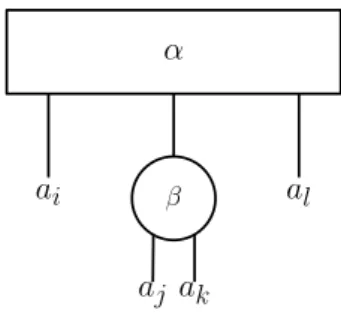
Figure 1: A P Q-tree
We define the set of orders LP, with B∈ LP if and only if the dataset P satisfies condition
(4) with respect to B. In this section, we will describe an algorithm which identifies this set LP.
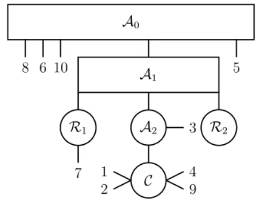
We will represent the set LP by a P Q-tree. This P Q-tree T on the set A represents a set of
permutations on A, corresponding to the orderings B∈ LP. The leaves ofT are the elements
of A and the nodes are of two types. A P -node (represented by circles) allows any permuta-tion of its children. On Q-nodes (represented by rectangles), the children are ordered and only reversals are allowed. For example, the P Q-tree in Figure 1 represents the set of permutations {(i, j, k, l), (i, k, j, l), (l, j, k, i)(l, k, j, i)}. For every node α of the P Q-tree, the set S(α) is the set of its children and this set can contain both alternatives as well as other nodes. The ordering of children of a P node is represented by [i B β B l], the brackets indicating that this order can
be reversed. The use of a P Q-tree allows us to efficiently represent LP, which may have an
exponential number of members.
In their paper on single-peaked orders Doignon and Falmagne [10] use a representation for the reference orders B for which a given preference profile is single-peaked. They represent these using nested ‘boxes’, where the order of alternatives within the same box can be reversed. Figure 2a is from an example in the Doignon and Falmagne paper, showing the reference orders consistent with a given preference profile using the ‘boxes’ representation. Figure 2b shows these same orders, represented by a P Q-tree.
(a) ‘Boxes’ representation
8
9
7 6
1
2
5
3
4
(b) P Q-Tree representation
Figure 2: Representations of reference orders B.
satisfied by each B ∈ LP. Specifically, these properties will allow us to identify an extreme
alternative, ¯a, which is either the first or last alternative in any ordering B ∈ LP. Next, the
main part of this section is the description of an algorithm which uses this information on extreme alternatives to determine the set LP in Section 4.2.
4.1
Preliminaries
Claim 1. For any B∈ LP and each triple of alternatives i, j, k∈ A:
if i B j B k then pij≤ pjk. (5)
Proof. Suppose this is not the case and pjk < pij. Condition (4) requires pij ≤ pik, thus
pjk < pik. Equivalently, 1− pkj< 1− pki or pkj> pki, which violates condition (4).
It is a well known result that if preferences are single-peaked, there exists one (or more)
Condorcet winner(s) [3]. A Condorcet winner is an alternative c∈ A, such that for every other
alternative i ∈ A, pci ≥ 0.5. Such a Condorcet winner must obviously exist for LP to be
non-empty. We next show that if there are multiple Condorcet winners, there can not be any
Condorcet non-winner in between two Condorcet winners in an ordering B∈ LP.
Claim 2. Consider two Condorcet winners, c, c0∈ A and an alternative i ∈ A, with c B i B c0.
If B∈ LP, i is also a Condorcet winner.
Proof. Since both c and c0 are Condorcet winners, pcc0 = 0.5 and both pic≤ 0.5 and pic0 ≤ 0.5.
By condition (5), 0.5≥ pic0 ≥ pci≥ 0.5, thus pic0 = 0.5 and by the same argument, pic = 0.5.
Furthermore, for any alternative j ∈ A with j B c B i (i B c0 B j), it must be the case that
pij ≥ pic = 0.5 (resp. pic0 = 0.5). Thus, for every alternative j ∈ A, pij ≥ 0.5 and i is a
Condorcet winner.
Claim 3. Consider an alternative i∈ A, such that for all Condorcet winners c ∈ A, pic= 0.5.
Then, if LP 6= ∅, the alternative i is also a Condorcet winner.
Proof. Consider a Condorcet non-winner j∈ A, and let c ∈ A be a Condorcet winner. If there
exists an ordering B∈ LP, one of the following three cases must be true. we show that in each
case pij ≥ 0.5. Since this is true for each j ∈ A, i must be a Condorcet winner.
• If j B i B c, we have pcj ≥ 0.5, as c is a Condorcet winner. By condition (5), pij ≥ pcj, so
pij≥ 0.5.
• If i B c B j, we have pic= 0.5 and by condition (4) we have pic≤ pij, so again pij ≥ 0.5.
• If i B j B c, we have pic= 0.5 and pic≤ pjc (condition (4)). It must thus also be the case
that pjc = 0.5. Note that if there are alternatives j for which i B j B c, there must exist
an alternative j0 with i B j0B c, for which there does not exist an alternative k∈ A such that j0B k B c. For this alternative, only the first two situations described apply, and thus pj0j ≥ 0.5 for all j ∈ A. j0 is thus also a Condorcet winner. By induction, if pic= 0.5 for
some Condorcet winner c, then for all alternatives j with i B j B c, j is a Condorcet winner. Since we start from the premise that pic= 0.5 for all Condorcet winners, pij = 0.5.
For every alternative i ∈ A, we define its Minimax score, minmax(i) = maxj∈Apji. This
value is the alternative’s greatest head-to-head defeat. In the following claim, we show that for
any ordering B∈ LP, minmax(i) = pji, with j the immediate neighbour of i to the side of the
Claim 4. Consider the alternative i ∈ A, a Condorcet winner c ∈ A and j ∈ A. For every B∈ LP, with i B j B c (or j is a Condorcet winner itself ) and for which there does not exist any
k∈ A for which i B k B j, it must be the case that:
minmax(i) = pji. (6)
Proof. Suppose this is not the case, then there exists an alternative l∈ A, such that pli > pji.
For this alternative, it must be the case that either i Bj Bl or l BiBj. The first case immediately contradicts condition (4). In the second case, condition (5) requires pil ≥ pji ≥ pcj ≥ 0.5 (if
j = c, pji≥ 0.5 is immediate). Thus, pli≤ 0.5 ≤ pji, another contradiction.
For the next claim, we first define a second value for every alternative. We denote the number
of head-to-head wins of an alternative by w(i), i.e., w(i) is the number of alternatives j ∈ A
for which pij > 0.5. We are now in a position to identify an extreme alternative. This is an
alternative which, for every B∈ LP is either the first or last alternative of this order.
Claim 5. If there exist an alternative that is not a Condorcet winner, then there exists an extreme alternative i∈ A, such that
1. i is not a Condorcet winner.
2. minmax(i) = maxj∈Aminmax(j).
3. For all other i0 ∈ A for which minmax(i0) = maxj∈Aminmax(j), w(i)≤ w(i0).
4. For every B∈ LP, it must be the case that this alternative i is either the first or the last
alternative (i.e. let c be a Condorcet winner, then there is no alternative j ∈ A such that c B i B j).
Before we give the proof, note that one of the requirements of an extreme alternative is that it is not a Condorcet winner. It can be easily checked that if no Condorcet non-winner exists, pij = 0.5 for all i, j ∈ A and every possible ordering B ∈ LP.
Proof. First, it can be easily checked that if there exists a Condorcet non-winner, an alternative satisfying the first three conditions must exist. Indeed, for a Condorcet non-winner i, there must be at least one Condorcet winner c∈ A for which pci> 0.5 (Claim 3). Since for any Condorcet
winner c and for every alternative j∈ A, pjc≤ 0.5, no Condorcet winner can satisfy the second
condition. In the remainder of the proof we argue that if there is an alternative i∈ A that does not satisfy the fourth condition, it also does not satisfy either the second or third condition.
To start, if there exists an ordering B∈ LP, there exists a Condorcet winner c∈ A, for which
pci > 0.5. Now suppose i is not an extreme alternative, i.e., there exists an ordering B ∈ LP
such that for some alternative j ∈ A, c B i B j. Let i0 ∈ A be the immediate neighbour of i
(c B i0B i), by condition (5) and claim 4, minmax(i) = p
i0i≤ pij ≤ minmax(j). Thus, either i
does not satisfy the second condition, or both i and j do. If i does satisfy the second condition, then w(i) > w(j). Indeed, consider k∈ A. If k B i B j, then pik≥ pjk (condition (4)). Second,
if c B i B k B j, because pci> 0.5, we have pik> 0.5 and pjk < 0.5 (condition (5)). In the third
situation, c B i B j B k, both pik > 0.5 and pjk > 0.5. Thus, whenever j is preferred to some
third alternative k, i is also preferred to it, so at least w(i)≥ w(j). Finally, because pij > 0.5,
4.2
The Algorithm
We are now in a position to describe our algorithm for identifying the set LP, represented by
a P Q-tree T . The main idea of this algorithm is as follows. First, we go through some
ini-tialization steps (Algorithm 2). Initially, all alternatives are assigned to a P -node A1, which
serves as a holding node from which the alternatives will later on be assigned to other parts of
the tree. Next, we identify an extreme alternative ¯a and Condorcet winners, these Condorcet
winners are assigned to a P -node C. Starting from the extreme alternative, we will split the
Condorcet non-winners into two groups (Algortihm 5). (In terms of the P Q-tree, we assign them to P -nodesR1 andR2.) The first group (nodeR1) are alternatives which must be on the same
side of the Condorcet winners as the initially identified extreme alternative in every B ∈ LP,
while the second group (node R2) is on the opposite side. We use a combination of two simple
subprocedures, Splitting 1 and 2 (Algorithms 3 and 4), to make this split. Given this split, the relative ordering of the alternatives in the two groups can easily be established based on the w(a) values (Algorithm 6). It is possible that not all Condorcet non-winners can be assigned to either of these two groups, and there remains a subset of alternatives as children ofA1. We show that
in this case, any ordering B0∈ LP0 over these children ofA1 can be used to complete the partial
ordering we have already found over the other alternatives. The final step is the ordering of the Condorcet winners (Algorithm 7).
Algorithm 1 shows an overview of the different procedures used.
Algorithm 1 IdentifyingT
1: Intialization ofT with nodes A0,A1,R1,R2,C (Algorithm 2).
2: while S(A1)6= {C} do
3: Splitting Procedure (Algorithm 5).
4: Ordering Condorcet non-winners (Algorithm 6).
5: if S(A1) ={C} then
6: Break
7: else
8: ChangeA1 into a Q-Node.
9: CreateR1,R2∈ S(A1) ([R1BC B R2]).
10: Identify an extreme alternative of S(A1).
11: In the following iteration of the loop, treat A1as the root node.
12: end if
13: end while
14: Ordering Condorcet winners (Algorithm 7).
Before we begin describing the algorithm in more detail, an important note. In the interest
of simplicity, the algorithm has been constructed under the assumption that LP 6= ∅. We will
show that if this assumption holds, the output, the P Q-tree T , represents the set LP. If this
assumption does not hold, there will still be an outputT . However, every ordering B consistent
with this tree will obviously violate condition (4) for the dataset P . As a result, we can tell
whether T represents LP or if LP = ∅ by testing condition (4) for a single ordering of the
alternatives.
We begin by describing the initialization steps of the algorithm. For each alternative i∈ A,
score, minmax(i). We also initialize the treeT . Initially, we assign all alternatives to the node
A1. This node has a child nodeC, to which all Condorcet winners are then assigned. Next, we
identify an extreme alternative ¯a and assign it to the nodeR1 and the set V , which will be used
later on in the algorithm. This set contains alternatives assigned to R1 or R2 which have not
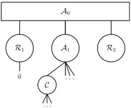
yet been used to sort other alternatives into these nodes. Figure 3 shows the P Q-tree after this initialization.
Algorithm 2 Initialization
1: Create T with root Q-node A0 and P -nodesR1,R2,A1,C.
2: Set S(A0) :={R1,R2,A1}, with [R1BA1BR2].
3: Set i∈ S(A1) for all i∈ A and C ∈ S(A1).
4: for all i∈ A do
5: Set w(i) :=|{pij > 0.5, j∈ A}|.
6: Set minmax(i) := maxj∈A(pji).
7: if minmax(i)≤ 0.5 then
8: Set S(C) := S(C) ∪ {i}, S(A1) := S(A1)\{i}.
9: end if
10: end for
11: Find an extreme alternative ¯a: minmax(¯a) = maxi∈A minmax(i) and w(¯a)≤ w(j) for all
j ∈ A for which minmax(¯a) = minmax(j)
12: Set S(R1) := S(R1)∪ {¯a}, S(A1) := S(A1)\{¯a}.
13: Set V := V ∪ {¯a}. A0 A1 . . . R1 ¯ a R2 C . . .
Figure 3: P Q-tree after Initialization
Starting from this single extreme alternative ¯a in S(R1), we will partition the other Condorcet
non-winners over the sets S(R1) and S(R2), using the procedures Splitting 1 and Splitting 2
(Algorithms 3 and 4). The main idea for the first procedure is simple. Consider, without loss of generality, i∈ S(R1) and j ∈ S(A1). Next, suppose pij < maxc∈C(pic), then i B c B j
vio-lates condition (4). Thus, for every B∈ LP, the alternative j must be on the same side of the
Condorcet winners as i. In this case, we set j∈ S(R1). Likewise, suppose pij > minc∈S(C)(pic).
Then the ordering i B j B c violates condition (4) and the options j B i B c and i B c B j remain.
In claim 6, we show that if there is an ordering B∈ LP with j B i B c, j would be assigned to
an R node before or in the same iteration as i. It follows that if j ∈ S(A1), i ∈ S(R1), and
pij > minc∈S(C)(pic), the alternative j must be on the other side of the Condorcet winners and
Claim 6. If there exists an ordering B∈ LP, two Condorcet non-winners j, k and one Condorcet
winner c, such that j B k B c, Splitting 1 will assign j to S(Rt) (t ={1, 2}) before, or during the
same iteration as, it assigns k to S(Rt).
Proof. Suppose an alternative i∈ V is chosen in step 2 of Splitting 1, for which there does not
exist an ordering B0 ∈ LP with j B0iB0c. First, notice that the existence of B∈ LP, with j BkBc
and the non-existence of B0∈ LP with j B0i B0c implies either i B j B k B c or j B k B c B i. Now,
suppose i is (without loss of generality) a member of S(R1). The alternative k is then assigned to
S(R2) if pik> minc∈S(C)(pic) or to S(R1) if pik< maxc∈S(C)(pic). In case pik> minc∈S(C)(pic),
the ordering i B j B k B c violates condition (4), so it must be the case that j B k B c B i. Then pij ≥ pik> minc∈S(C)(pic) and both j and k are assigned to S(R2). If pik< maxc∈S(C)(pic), the
same reasoning holds. An ordering j B k B c B i violates condition (4), so it must be the case that i B j B k B c. Condition (4) then requires that pij ≤ pik< maxc∈S(C)and both alternatives
are assigned to S(R1).
This line of reasoning hinges on the choice of an alternative i∈ V in step 2, for which there does not exist an ordering B0 ∈ LP with j B0i B0c (for all j∈ S(A1)). In the first iteration, this
is guaranteed because i will be an extreme alternative. In later iterations, this property follows
from induction. If there was an ordering B∈ LP with j B i B c, both j and i would have been
assigned to either S(R1) or S(R2) and j /∈ S(A1).
Algorithm 3 Splitting 1
1: while V 6= ∅ do
2: Choose an i∈ V .
3: Set r such that i∈ S(Rr).
4: for all j∈ S(A1) do
5: if pij > minc∈S(C)(pic) then
6: Set S(R3−r) := S(R3−r)∪ {j}.
7: Set S(A1) := S(A1)\{j}.
8: else if pij< maxc∈S(C)(pic) then
9: Set S(Rr) := S(Rr)∪ {j}. 10: Set S(A1) := S(A1)\{j}. 11: end if 12: end for 13: Set V := V\{i}. 14: end while
It is possible that this procedure ends before all Condorcet non-winners have been assigned to sets S(R1) or S(R2). In the next claim, we show this can only happen in a specific situation.
Claim 7. If Splitting 1 ends before all Condorcet non-winners have been assigned to sets S(R1)
or S(R2), then for every alternative i∈ S(R1)∪ S(R2) and every pair of alternatives j, j0 ∈
S(A1)∪ S(C), it must be the case that pij = pij0.
Proof. We argue as follows, suppose that at the end of Splitting 1, there exists an alternative i ∈ S(R1)∪ S(R2) for which there is a pair j, k ∈ S(C) such that pij 6= pik. In this case,
Splitting 1 can assign at least one more alternative in S(A1) to either S(R1) or S(R2). First,
assume there exist two alternatives j, k ∈ S(C), such that pij > pik. Then for any Condorcet
the second pil > minc∈S(C)(pic). In either case, l would get sorted into either S(R1) or S(R2).
Next, suppose that pij = pik for all j, k∈ S(C), then there is some l ∈ S(A1) for which pil6= pic
for all c∈ S(C). It follows that either pil< maxc∈S(C)(pic) or pil> minc∈S(C)(pic) and l would
get sorted.
In this case we turn to a second splitting procedure. Consider two alternatives i, j ∈
S(A1)∪ S(C), with minmax(i) = pji. Through Claim 4, we know that for any B ∈ LP,
i B j B c, with c a Condorcet winner (or j is itself a Condorcet winner). Now consider an alter-native k ∈ S(Rr), with pjk < pji, then k B i B j B c violates Condition (4) and we must have
k BcBj Bi. In other words, we know i must be on the other side of the Condorcet winners than k. Searching through all possible triples i0, j0 ∈ S(A1)∪ S(C) and k0 ∈ S(Rr) is not very
efficient. In Splitting 2, we therefore make use of some previous claims to quickly identify
potential violations. Specifically, we use these to find alternatives i, j ∈ S(A1)∪ S(C) and
k ∈ S(Rr) such that pjk = minj0∈S(A
1)∪S(C),k0∈S(Rr)pj0k0 and pji = maxi0,j0∈S(A1)∪S(C)pj0i0.
Clearly, if this triple does not have pjk < pji, there doesn’t exist any such triple. First, we
identify an extreme alternative ¯a of the set S(A1) using Claim 5. It is a property of extreme
alternatives that minmax(¯a) = maxi0∈S(A
1)minmax(i
0). Furthermore, we have the following
claim.
Claim 8. Consider the set S(A1) of Condorcet non-winners not assigned in Splitting 1. If there
exists an ordering .∈ LP then maxi,j∈S(A1)∪S(C)pji= maxi∈S(A1)minmax(i).
Proof. Suppose this is not the case, then there must be some alternative k ∈ S(R1)∪ S(R2),
such that pki= minmax(i). As i is a Condorcet non-winner, minmax(i) > 0.5. In claim 7, we
have shown that for every k∈ S(R1)∪ S(R2), pkj= pkj0 for every distinct pair of alternatives
j, j0 ∈ S(A
1)∪ S(C). This implies that for all Condorcet winners c ∈ S(C), pki = pkc >
0.5, which is not possible. Thus, for every i ∈ S(A1), maxj∈S(A1)∪S(C)pji = minmax(i) and
maxi,j∈S(A1)∪S(C)pji= maxi∈S(A1)minmax(i).
Second, we compute mink0∈S(R
r)p¯ak0 for both r = 1, 2 and we denote this value by p(Rr).
Through Claim 7, we know that p¯ak0 = pj0k0 for all j0∈ S(A1)∪ S(C), thus p(Rr) =
mink0∈S(Rr),j0∈S(A1)∪S(C)pj0k0. We can now check whether p(Rr) < minmax(¯a). If this is the
case, adding the alternative ¯a to S(Rr) leads to violations and we add ¯a to the opposite set.
Algorithm 4 Splitting 2
1: Find the extreme alternative ¯a of S(A1).
2: Set p(R1) := mini∈S(R1)(pai¯). 3: Set p(R2) := mini∈S(R2)(pai¯). 4: if minmax(¯a) > p(R1) then
5: Set S(R2) := S(R2)∪ {¯a}.
6: Set S(A1) := S(A1)\{¯a}.
7: Set V := V ∪ {¯a}.
8: else if minmax(¯a) > p(R2) then
9: Set S(R1) := S(R1)∪ {¯a}.
10: Set S(A1) := S(A1)\{¯a}.
11: Set V := V ∪ {¯a}.
Note that by assigning the extreme alternative of S(A1) in Splitting 2, we ensure Claim 6
re-mains valid. Indeed, this ensures that at no point is there a triple of two Condorcet non-winners
i, j and a Condorcet winner c, with i B j B c for some B∈ LP where j is already assigned to
either S(R1) or S(R2) while i is not.
If Splitting 2 can assign an alternative to eitherR1orR2(in which case V is no longer empty),
we can return to Splitting 1. If at any point, Splitting 1 again terminates without having sorted all Condorcet non-winners, Splitting 2 is again used, and so on. Algorithm 5 summarizes the complete Splitting Procedure.
Algorithm 5 Splitting Procedure
1: Initialization 2: while V 6= ∅ do 3: Splitting 1 4: if S(A1)6= {C} then 5: Splitting 2 6: end if 7: end while
After the splitting procedure finishes, the alternatives assigned toR1andR2will be ordered.
By construction of these sets, any two alternatives i, j ∈ S(Rr) must be placed to the same
side of any alternative c∈ S(C). Their relative ordering, i.e., which alternatives must be placed
closest toC, can be determined by the values of w(i) as shown in the following claim.
Claim 9. If LP 6= ∅, then for any two Condorcet non-winners i, j ∈ S(Rr), w(i)6= w(j) and a
Condorcet winner c∈ S(C), w(i) < w(j) if and only if for any B ∈ LP it is the case that i B j B c
or c / j / i.
Proof. For all k with i B j B k, we have pjk> pik, so j has at least as many wins against
alterna-tives the its right as i has. For all k6= i with k B j B c, we have pjk> 0.5 (since pck> 0.5), so j
also has at least as many wins against alternatives to its left as i has. Finally, because pci> 0.5
we have pji> 0.5, so j wins head-to-head against i, which gives at j at least one more win than i.
Suppose w(i)≥ w(j), then there should be either at least one alternative k such that both
pik> 0.5 and pjk≤ 0.5 or it should be the case that pij = 0.5. However, by the same arguments
as above neither situation can occur.
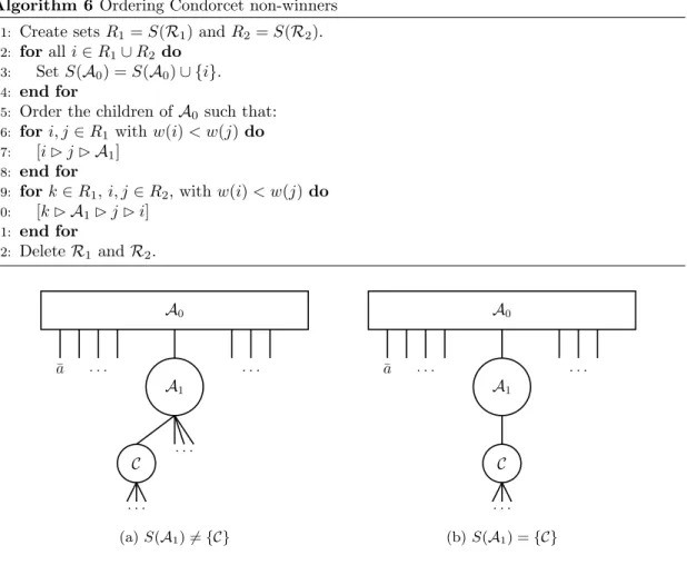
At this point, we are either in the situation depicted in Figure 4a or the one given in Figure 4b.
Let us first consider the case with S(A1) 6= {C}, depicted in Figure 4a. We have shown in
Claim 7 that if Splitting 1 terminates with S(A1) 6= {C}, then for any given i ∈ S(A0) and
every pair j, j0 ∈ S(A
1)∪ S(C), the values pij = pij0. Thus both [i B j B j0] and [i B j0B j] are
allowed. Furthermore, if the splitting procedure ends with S(A1)6= {C}, then Splitting 2 has
run without finding a pair j, j0 ∈ S(A1)∪ S(C) and alternative i ∈ S(R1)∪ S(R2), such that
pjj0> pji. This again allows both [i B j B j0] and [i B j0B j]. Combining these two observations,
it is clear that no matter how we order the children of S(A1), no new violations of condition (4)
involving alternatives both in S(A0) and S(A1)∪ S(C) can be created. A1 can thus be handled
independently of the other alternatives. This is done by changing A1 into a Q-node, creating
Algorithm 6 Ordering Condorcet non-winners
1: Create sets R1= S(R1) and R2= S(R2).
2: for all i∈ R1∪ R2 do
3: Set S(A0) = S(A0)∪ {i}.
4: end for
5: Order the children ofA0 such that:
6: for i, j∈ R1with w(i) < w(j) do
7: [i B j BA1]
8: end for
9: for k∈ R1, i, j∈ R2, with w(i) < w(j) do
10: [k BA1B j B i] 11: end for 12: Delete R1 andR2. A0 ¯ a . . . . A1 . . . C . . . (a) S(A1) 6= {C} A0 ¯ a . . . . A1 C . . . (b) S(A1) = {C}
Figure 4: Possible states after the Condorcet non-winners have been ordered.
situation can reoccur at most O(n) times. Each time the algorithm is run, at least one alterna-tive (the extreme alternaalterna-tive), becomes a direct child of the Q-nodeA0,A1, . . .. Eventually, the
second situation will occur.
Next, we consider the case depicted in 4b. In this case, the nodeA1is deleted andC is made a
direct child ofA0. Since all children ofC are Condorcet-Winners, pcc0 = 0.5 for all c, c0 ∈ S(C). It
is therefore clear that no violation of condition (4) can exist involving only alternatives in S(C).
The relative ordering of alternatives in S(C) is thus determined by alternatives outside of C.
Algorithm 7 provides the full pseudo-code for finding this ordering. The main idea is as follows; we look for alternatives i∈ S(A0), for which there exist two alternatives c, c0 ∈ S(C) such that
pic0 > pic. The nodeC is then replaced by three P -nodes, C1,C2,C3. Alternatives j ∈ S(C) are
divided over these three nodes, based on whether pic≥ pij (C1), pic0> pij> pic(C2) or pij≥ pic0
(C3). These nodes are ordered such that [i BC1BC2BC3]. It is clear that any other ordering
of these nodes would allow violations of Condition (4). If these new nodes have more than one child, they can be split in the same manner. This process of splitting P -nodes continues until either all of these nodes contain only one child, or until no more nodes can be split. We again use a set V in this algorithm, which contains all alternatives in S(A0) which can potentially be used
to split one of the P -nodes. This set will be important later in the time analysis of the algorithm.
Algorithm 7 Ordering Condorcet winners
1: Set V := S(A0)\{C}.
2: while V 6= ∅ and there exist a P -node Cj with|S(Cj)| > 1 do
3: Choose i∈ V .
4: if There does not exist a P -nodeCj, with c, c0∈ S(Cj) and pic0 > picthen
5: Set V := V\{i}.
6: else
7: for all P -nodesCj, with c, c0 ∈ S(Cj) and pic0 > picdo
8: Create P -nodesCj,1,Cj,2,Cj,3 ∈ S(A0) with [i BCj,1BCj,2BCj,3]
9: for all k∈ S(Cj) do 10: if pik≥ pic0 then 11: Set S(Cj,3) := S(Cj,3)∪ {k}. 12: else if pic0 > pik> pic then 13: Set S(Cj,2) := S(Cj,2)∪ {k}. 14: else 15: Set S(Cj,1) := S(Cj,1)∪ {k}. 16: end if 17: end for 18: Delete node Cj. 19: end for 20: end if 21: end while
22: for all P -nodes Cj with|S(Cj)| = 0 do
23: Delete node Cj.
24: end for
25: for all P -nodes Cj with|S(Cj)| = 1 do
26: Delete node Cj, replace it by its child in the ordering ofA.
27: end for
As mentioned earlier, we must still test the output of Algorithm 1. We take one ordering B
consistent with the P Q-tree T and test whether condition (4) holds. If this ordering satisfies
the condition, obviously LP 6= ∅. We will now show that if LP 6= ∅, the P Q-tree T represents
LP. This also implies that if B does not satisfy the condition (4), LP is an empty set. Indeed,
if LP 6= ∅, every ordering consistent with T satisfies the condition (4).
Theorem 3. If the set LP 6= ∅, then Algorithm 1 constructs a P Q-tree T , representing LP.
Proof. To prove this theorem, we must show two things to be true:
(i) All restrictions on the ordering consistent with the treeT are necessary to avoid violations of Condition (4).
(ii) No ordering consistent with the treeT violates Condition (4).
Throughout the description of the algorithm, we argue (i) is true. Whenever a subroutine of the algorithm fixes the relative ordering of alternatives, we argue that allowing any other relative ordering of these alternatives leads to violations of Condition (4). For brevity, we will only sum-marize these arguments in this proof. To show (ii) is true, we must show that whenever there
is more than one possible relative ordering for a triple of alternatives consistent withT , all of these relative orders satisfy Condition (4).
Let us begin by summarizing the arguments for (i). The subroutines Splitting 1, Splitting 2, Ordering of Condorcet non-winners and Ordering of Condorcet Winners, are used to build the tree T . If these routines only fix the relative ordering of alternatives to eliminate possible violations of Condition (4), then (i) is satisfied. We first look at Splitting 1. This routine begins with an extreme alternative, which must be either the first or the last alternative in any ordering
B∈ LP (Claim 5). We then identify potential violations of Condition (4) involving the extreme
alternative, a Condorcet winner and a Condorcet non-winner. If such a potential violation is found, the Condorcet non-Winner is fixed to a side of the Condorcet winners, so that the relative
ordering leading to the potential violation is no longer consistent with T . Once the Condorcet
non-winner is fixed to a side, Splitting 1 can use it to identify other potential violations. The main text shows how these potential violations are found. Claim 6 further supports the cor-rectness. Splitting 2 works in a similar way, again we look for potential violations of Condition (4). In this routine, we identify potential violations involving one alternative already assigned to S(R1) (or S(R2)) and 2 alternatives in S(A1) or S(C). Again, we show how to identify these
potential violations in the main text and argue how re-assigning one alternative to S(R1) or
S(R2) is necessary to avoid it. The ordering of Condorcet non-Winners is based on their w(i)
values. Claim 9 proves the correctness of the procedure. Finally, the Ordering of Condorcet win-ners is again based on identify potential violations, this time involving two Condorcet winwin-ners and one Condorcet non-winner. Again, the main text shows how these potential violations can be identified and how the tree can be ordered to avoid these.
We have now summarized the arguments that show any relative orders imposed by the treeT
are necessary to avoid violations of Condition (4). It remains to be shown that there is no need for any additional restrictions, i.e., all relative orders consistent with T satisfy Condition (4). The figure 5 is used to illustrate the arguments made to do so. The figure shows the structure of a treeT at the end of the algorithm. This tree T consists of a root Q-node A0, whose direct
children are Condorcet non-winners and one Q-node A1. A node with this group of children
is formed if the situation in Figure 4a occurs. The children of A1 are choice alternatives, both
Condorcet winners and non-winners, and P -nodesC1 andC2, this group of children is formed if
the situation in Figure 4b occurs.
A0 A1 C1 C2 ai aj ad ae af ag ah ak al ap aq
There are three cases were, for a triple of alternatives, multiple relative orders are allowed. First, this can happen if there is there is one direct child ofA0and 2 children (direct or indirect)
of A1. Note that A1 is only kept in the tree T if after Splitting 1 and Splitting 2, we have
S(A1) 6= C, the situation depicted in figure 4a. We have already argued that if this situation
occurs, there can be no violation involving a triple with alternatives in both S(A0) and S(A1).
A second case is if there is a Condorcet non-winner i∈ S(A1) and two Condorcet winners j, k,
direct children of the nodeClnode. It can be quickly checked that if pij 6= pik, the nodeClwould
have been split in the Ordering of Condorcet winners routine. Thus, pij = pik and both relative
orders consist with T satisfy Condition (4). Finally, there are several cases where a triple of
Condorcet winners allows multiple relative orderings of the alternatives. None of the relative orderings of these triples can be violations of Condition (4), since for any two Condorcet winners c, c0, it must be the case that pcc0 = 0.5.
Let us now turn to the analysis of the time complexity of this algorithm. We claim and prove the following result.
Theorem 4. Algorithm 1 runs in O(n2) time.
Proof. We begin with the initialization procedure. For a given alternative i, the values of w(i)
and minmax(i) can be computed by checking all elements of the ith row and column of the
pij-matrix (O(n) elements). While reading these values, it can also be determined whether i is
a Condorcet winner. Computing these values for all alternatives and determining the Condorcet
winners thus takes O(n2)-time. Identifying an extreme alternative can be done by checking the
minmax(i) and w(i) values for all alternatives once (O(n)), and thus the complexity of the com-plete initialization procedure is bounded by O(n2).
Next, we turn to the splitting procedures (Splitting 1 and Splitting 2). Notice that for every alternative i∈ A, the main loop of Splitting 1 (lines 4-11) is run at most once. In this loop, the
value pij for all elements j ∈ S(A1) is checked and a constant number of operations performed
based on this value. The O(n) iterations of the loop in Splitting 1, and the O(n) operations in
this loop provide an upper bound of O(n2) operations for the Splitting 1 procedure throughout
the algorithm. Likewise, Splitting 2 is used at most O(n) times. The three most costly steps are contained in lines 1-3, and in each case, at most O(n) values must be checked. In particular, for line 1, there are O(n) values minmax(i) to be compared. In line 2 and line 3, for a given
alternative j ∈ S(A1), the pji values must be checked, of which there are again O(n). Since
Splitting 2 is run at most O(n) time and takes at most O(n) time for each iteration, the total time spent on Splitting 2 is also at most O(n2).
The time complexity of ordering the Condorcet non-winners (Algorithm 6) is straightforward. In this procedure, alternatives which are a child of the same node (R1 orR2) are ordered based
on their w(i) values. For m alternatives, ordering can be done in O(m log(m)) time. Since each alternative is ordered in only one iteration of this procedure, the total time spent order-ing Condorcet non-winner alternatives is less than O(n log(n)). Finally, Algorithm 7 orders the
Condorcet winners. In line 3, an alternative i∈ V is chosen and one of two cases will be true.
Either there is a P -node Cj, with c, c0 ∈ S(Cj) and pic0 > pic, or there is not. Determining
which of the two situations is relevant takes O(n) time, since this can be done by determining the minimum and maximum pij values. If no node with c, c0 ∈ S(Cj), pic0 > pic exists, the if
statement resolves in constant time. If there is such a node, the else procedure resolves, which
and maximum determined earlier. Given this, it is clear that after choosing an i∈ V , it takes at most O(n) time to resolve the if-else procedure. Next, notice that this if-else procedure is run at most O(2n) times. Indeed, if no node with c, c0 ∈ S(Cj), pic0 > pic exists, i is removed from
the set V . If this situation occurs O(n)) times, the set V is empty and the algorithm stops. If such a node exists, at least one P -node will be split into at least two parts. Since there are at most n alternatives in S(C) at the start, it must be the case that after n splits, each Cj node
has only 1 child. Since one iteration of the if-else procedure takes O(n) time and there can be
at most O(n) iterations, ordering the Condorcet winners happens in O(n2) time.
In conclusion, we have shown that at most O(n2) time is spent in each of the procedures, as a result, the total running time of the algorithm is also bounded by O(n2).
4.3
An Example
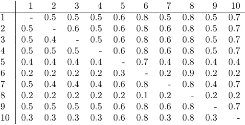
In this section, we will illustrate the algorithm described in this section with an example. Table 1 shows the pij values for all pairs of alternatives.
1 2 3 4 5 6 7 8 9 10 1 - 0.5 0.5 0.5 0.6 0.8 0.5 0.8 0.5 0.7 2 0.5 - 0.6 0.5 0.6 0.8 0.6 0.8 0.5 0.7 3 0.5 0.4 - 0.5 0.6 0.8 0.6 0.8 0.5 0.7 4 0.5 0.5 0.5 - 0.6 0.8 0.6 0.8 0.5 0.7 5 0.4 0.4 0.4 0.4 - 0.7 0.4 0.8 0.4 0.4 6 0.2 0.2 0.2 0.2 0.3 - 0.2 0.9 0.2 0.2 7 0.5 0.4 0.4 0.4 0.6 0.8 - 0.8 0.4 0.7 8 0.2 0.2 0.2 0.2 0.2 0.1 0.2 - 0.2 0.2 9 0.5 0.5 0.5 0.5 0.6 0.8 0.6 0.8 - 0.7 10 0.3 0.3 0.3 0.3 0.6 0.8 0.3 0.8 0.3
-Table 1: Matrix of pij-values.
Initialization
We compute the head-to-head wins and minimax scores for each alternative. Results are given in Table 2.
1 2 3 4 5 6 7 8 9 10
minmax(i) 0.5 0.5 0.6 0.5 0.6 0.8 0.6 0.9 0.5 0.7
w(i) 4 6 5 5 2 1 4 0 5 3
Table 2: Head-to-head wins and Minimax Score.
From these values, we see that 1, 2, 4 and 9 are Condorcet winners, we set S(C) = {1, 2, 4, 9}.
The alternative 8 is an extreme alternative, as minmax(8) = maxi∈Aminmax(i) and there are
no other alternatives for which this is the case. We set S(R1) = {8} and V = {8}. All other
alternatives are direct children ofA1. Figure 6a depicts the tree after the initialization.
Splitting Procedure - Splitting 1
Given the extreme alternative 8 and the Condorcet winners 1, 2, 4, 9, we use Splitting 1 to place Condorcet non-winners at the different sides of the Condorcet winners.
A0 A1 3 5 6 10 7 C 1 2 4 9 R1 8 R2
(a) Tree after Initialization
A0 A1 3 7 C 1 2 4 9 R1 8 6 10 R2 5
(b) Tree after Splitting
Figure 6
• We choose 8 ∈ V .
– For 6, we have p86< minc∈S(C)p8c.
∗ We set S(A1) := S(A1)\{6}, S(R1) := S(R1)∪ {6} and V := V ∪ {6}.
– For i = 3, 5, 7, 10, we have p8i = minc∈S(C)p8c= maxc∈S(C)p8c.
– Set V := V\{8}.
• We choose 6 ∈ V .
– For 5, we have p65> maxc∈S(C)p6c.
∗ We set S(A1) := S(A1)\{5}, S(R2) := S(R2)∪ {5} and V := V ∪ {5}.
– For i = 3, 7, 10, we have p6i= minc∈S(C)p6c= maxc∈S(C)p6c.
– Set V := V\{6}.
• We choose 5 ∈ V .
– For i = 3, 7, 10, we have p5i= minc∈S(C)p5c= maxc∈S(C)p5c.
– Set V := V\{5}.
At this point V = ∅ and we turn to the second splitting procedure. Splitting Procedure - Splitting 2
The extreme alternative of S(A1) is 10, since minmax(10) = maxk∈S(A1)minmax(k) = 0.7, and
for all other alternatives in S(A1) this is not the case.
• We compute pR1 = 0.8, pR2 = 0.6.
• Because minmax(10) = 0.7 > pR2.
– Set S(A1) := S(A1)\{10}, S(R1) := S(R1)∪ {10} and V := V ∪ {10}.
The algorithm now returns to Splitting 1, but is not able to assign any other alternatives to eitherR1 orR2. Figure 6b shows the tree at the end of the splitting procedures.
Ordering Condorcet non-winners
S(R1) now contains three alternatives, S(R2) only one. These nodes are removed and their
children are added to S(A0). We first order the alternatives that were in S(R1), based on their
head-to-head wins (w(i) values). The only alternative that was in S(R2), 5, is placed on the
other side ofA1. This leads to the ordering
[8 . 6 . 10 .A1. 5].
Figure 7a shows the tree at the end of the Condorcet non-winner ordering procedure.
A0 A1 3 7 C 1 2 4 9 8 6 10 5
(a) Tree after ordering Condorcet non-Winners A0 A1 A2 3 R1 7 R2 C 1 2 4 9 8 6 10 5
(b) Tree after re-initialization
Figure 7
Re-Initialization
We are now in the situation depicted in Figure 4a, i.e., the set S(A1)6= {C}. We re-run the
algorithm, now treatingA1as the root node. We chanceA1into a Q-node, and we createA2,R1
andR2, setting S(A1) :={R1,R2,A2}. All alternatives that were direct children of A1are made
direct children of A2. The minmax(i) and w(i) values computed earlier are re-used, and the
Condorcet winners also do not change. We identify a new extreme alternative for A1. We see
that minmax(3) = minmax(7) = maxi∈S(A1)minmax(i), and since w(7) < w(3), alternative
7 is that extreme alternative. We set S(R1) := {7} and V := {7}. The tree at this point is
depicted in Figure 7b.
Splitting Procedure - Splitting 1 • We choose 7 ∈ V .
– For 3, we have p73< minc∈S(C)p7c.
∗ We set S(A2) := S(A2)\{3}, S(R1) := S(R1)∪ {3} and V := V ∪ {3}.
– Set V := V\{7}.
At this point, S(A2) ={C}. Running the loop of Splitting 1 for 3 has no effect. We also do
not run Splitting 2.
Ordering Condorcet non-winners
children are added to S(A1). We order the alternatives that were in S(R1), based on their
head-to-head wins (w(i) values). This leads to the ordering [7 . 3 .A2].
Figure 8a shows the tree at the end of the Condorcet non-winner ordering procedure. At this
point, we are in the situation depicted in Figure 4b, we delete the nodeA2 and makeC a direct
child ofA1, we continue by using Algorithm 7.
Ordering Condorcet winners • Set V := {3, 7}.
• We choose 3 ∈ V
– We find for 1, 2∈ C that p3,1 = 0.5 > 0.4 = p3,2.
– We create P -nodeC1,C2,C3∈ S(A1), ordered [3 .C1.C2.C3].
– Since p3,1= p3,4 = p3,9= 0.5, we set S(C3) :={1, 4, 9}.
– Since p3,2= 0.4, we set S(C1) ={2}.
– We deleteC.
• We again choose 3 ∈ V .
– We do not find a nodeCi with two children j, k for which p3j6= p3k.
– We set V := V\{3}.
• We choose 7 ∈ V .
– We find for 1, 4∈ C3 that p7,1= 0.5 > 0.4 = p7,4.
– We create P -nodeC3,1,C3,2,C3,3∈ S(A1), ordered [7 .C3,1.C3,2.C3,3].
– Since p7,1= 0.5, we set S(C3,3) :={1}.
– Since p7,4= p7,9 = 0.4, we set S(C3,1) ={4, 9}.
– We deleteC3.
• We again choose 3 ∈ V .
– We do not find a nodeCi with two children j, k for which p7j6= p7k.
– We set V := V\{7}.
Figure 8b shows the final treeT , after all nodes with no or only one child have been deleted. Table 3 is a re-ordered version of Table 1, with the rows and columns re-ordered to show one ordering of the alternatives with the treeT . We see that it satisfies Condition 4.
A0 A1 7 3 A 2 C 1 2 4 9 8 6 10 5
(a) Tree after ordering Condorcet non-winners of A1 A0 A1 7 3 2 C 3,1 1 4 9 8 6 10 5
(b) Tree after ordering Condorcet winners
Figure 8 8 6 10 7 3 2 4 9 1 5 8 - 0.1 0.2 0.2 0.2 0.2 0.2 0.2 0.2 0.2 6 0.9 - 0.2 0.2 0.2 0.2 0.2 0.2 0.2 0.3 10 0.8 0.8 - 0.3 0.3 0.3 0.3 0.3 0.3 0.6 7 0.8 0.8 0.7 - 0.4 0.4 0.4 0.4 0.5 0.6 3 0.8 0.8 0.7 0.6 - 0.4 0.5 0.5 0.5 0.6 2 0.8 0.8 0.7 0.6 0.6 - 0.5 0.5 0.5 0.6 4 0.8 0.8 0.7 0.6 0.5 0.5 - 0.5 0.5 0.6 9 0.8 0.8 0.7 0.6 0.5 0.5 0.5 - 0.5 0.6 1 0.8 0.8 0.7 0.5 0.5 0.5 0.5 0.5 - 0.6 5 0.8 0.7 0.4 0.4 0.4 0.4 0.4 0.4 0.4
-Table 3: Ordered Matrix of pij-values.
5
Model Power
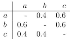
An important consideration for any test of choice behaviour is its power. If decisions made using other choice processes often generate datasets which satisfy the test conditions, the test has little value. Indeed, in this case there is no way of telling whether a positive test is the result of a correct hypothesis or just random chance. In this section, we briefly investigate the power of the tests we have described. Obviously, the test can not perfectly discriminate between single-peaked and non-single-peaked preferences. It is possible that the rates of choice of a non-single-peaked population still satisfy the conditions imposed by the mixture model with single-peaked preferences. Consider for example the following preferences and probabilities.
a 1c 1b x1= 0.4
b 2c 2a x2= 0.4
b 3a 3c x3= 0.2
It is clear that these preferences are not single-peaked. Given the probabilities for each preference ordering, we obtain the pij values in Table 4, which satisfy Condition (4).
a b c
a - 0.4 0.6
b 0.6 - 0.6
c 0.4 0.4
-Table 4: pij values satisfying Condition (4).
that a non-single-peaked population will satisfy them. We do so by comparing the volumes of the polytopes described by the conditions of the mixture model with single-peaked preferences against the volume of the linear ordering polytope. We represent these volumes as a percentage
of the volume of the complete sample space, an n2/2 dimensional hypercube with edge length 1,
each dimension corresponds to a pair of alternatives. ([27, 28]).
Exact computation of the volume of polytopes is a difficult task. Instead, we estimate them by uniform sampling from the complete sample space and testing them against the conditions imposed by single-peaked and linear ordering polytopes. The percentage of sampled datasets satisfying the conditions is an estimate for the volume of the associated polytopes. By limiting ourselves to five alternatives, we only have to check the triangle-inequalities for the linear ordering polytope [4, 22]. For single-peaked polytopes, we implemented the algorithm described in section 4. Since this algorithm may return an ordering for which the mixture model with single-peaked preferences is not satisfied (if such orders do not exist), we then checked the conditions of the mixture model. The result is the volume of the union of the single-peaked preference polytopes for all orderings of the alternatives. We also report an estimate of the volume of the single-peaked preference polytope for a given ordering. All of these results are given in table 5.
Linear Ordering Polytopes Union of Single-Peaked Polytopes Single-Peaked Polytope
n = 3 66.728% 49.999% 16.704%
n = 4 25.152% 3.3509% 0.2814%
n = 5 4.8975% 0.0208% 0.0007%
Table 5: Volumes of the Linear Ordering and Single-Peaked Polytopes for n = 3,4,5 It is clear that the mixture model with single-peaked preferences is highly restrictive. Even if we make the assumption that decisions are based on non-single-peaked preference orderings, there is a very low probability that the resulting choices are consistent with the mixture model for single-peaked preferences. For n = 5, this probability is already less than 0.5% if the union of all single-peaked polytopes is considered and it is clear that this probability quickly decreases
as n grows larger. Note that the estimated volume for the single-peaked polytope is about n!2
times the volume of the union of single-peaked polytopes. This must be the case as it can easily be seen that the polytopes for two different orderings B, B0are either equal, if B is the reverse of B0, or do not overlap. Indeed, if a dataset P satisfies the mixture model for both B, B0, B6= /0,
then it must satisfy a constraint of both with equality and as such the dataset is on the border of both.
6
Conclusions
In this paper, we presented a mixture model from the choice behaviour literature and applied it to a well-known choice domain from the social choice literature. Necessary and sufficient
conditions, first derived by Dridi [12], are described for the mixture model to hold for single-peaked preferences and a given ordering of the alternatives. We also showed that these conditions are easy to check in polynomial time, in contrast to the mixture model for general preferences. Furthermore, a polynomial time algorithm is provided to identify whether or not there exists some ordering of the alternatives for which the mixture model is satisfied. We also show that the conditions imposed on data by this model are very restrictive.
6.1
A Possible Extension
As single-peakedness is a very strong condition, it is generally recognized in the literature that populations are seldom truly single-peaked. Even if a logical ordering exists of alternatives, there will often be some agents whose preferences are based on very different criteria. For this reason, increasing attention is paid to notions of near-single-peakedness [16]. The mixture model as described in this paper could be extended to allow a limited number of states (weighted by probability) or percentage of the population to hold non-single-peaked preferences. For example, suppose we wish to test whether at most a fraction y of the population holds a non-single-peaked preference. Let O be the set of all strict preference orderings.
X m∈Oij xm= pij, ∀(i, j) ∈ A2, i6= j. (7) X m∈OB xm≥ 1 − y (8)
Another possibility is to test a mixture model where all preference orders are close to
single-peaked according to some measure. For example, any preference order for which a limited
number of switches of alternatives give a single-peaked order. Note that in the limit, these models suggested here become mixture models for general preference orders. Indeed, if y = 1, or the number of allowed switches is sufficiently high this is the case. Since the general mixture model is hard to test, it seems likely that testing such nearly-single-peaked mixture models will also turn out to be a hard problem.
7
Acknowledgements
I thank the two anonymous referees for their comments on this paper, and the action editor, Jean-Paul Doignon, for pointing me to the paper by Dridi and his other comments. Further-more, I would like to thank the members of my doctoral committee for their comments on an earlier version of this paper.
This research has been partially funded by FWO grant G.0447.10, and by the Inter-university Attraction Poles Programme initiated by the Belgian Science Policy Office.
References
[1] M. Ballester and G. Haeringer. A characterization of the single-peaked domain. Social Choice and Welfare, 36(2):305–322, 2011.
[2] J. Bartholdi III and M. Trick. Stable matching with preferences derived from a psychological model. Operations Research Letters, 5(4):165–169, 1986.
[3] D. Black. On the rationale of group decision-making. The Journal of Political Economy, 56(1):23, 1948.
[4] H.D. Block and J. Marschak. Random orderings and stochastic theories of responses. Con-tributions to probability and statistics, 2:97–132, 1960.
[5] K. Booth and G. Lueker. Testing for the consecutive ones property, interval graphs,
and graph planarity using pq-tree algorithms. Journal of Computer and System Sciences, 13(3):335–379, 1976.
[6] R. Bredereck, J. Chen, and G. Woeginger. Are there any nicely structured preference profiles nearby? Mathematical Social Sciences, 79:61–73, 2016.
[7] J. Christophe, J.P.L. Doignon, and S.L. Fiorini. The biorder polytope. Order, 21(1):61–82, 2004.
[8] C. Davis-Stober. A lexicographic semiorder polytope and probabilistic representations of choice. Journal of Mathematical Psychology, 56(2):86–94, 2012.
[9] C. Davis-Stober, S. Park, N. Brown, and M. Regenwetter. Reported violations of
ratio-nality may be aggregation artifacts. Proceedings of the National Academy of Sciences,
113(33):E4761–E4763, 2016.
[10] J. Doignon and J. Falmagne. A polynomial time algorithm for unidimensional unfolding representations. Journal of Algorithms, 16(2):218–233, 1994.
[11] T. Dridi. Sur les distributions binaires associ´ees `a des distributions ordinales. Math´ematiques et Sciences Humaines, 69:15–31, 1980.
[12] T Dridi. Distributions binaires unimodales. Discrete Mathematics, 126(1-3):373–378, 1994. [13] E. Elkind and P. Faliszewski. Recognizing 1-euclidean preferences: An alternative approach.
In SAGT, 2014.
[14] G. Erd´elyi, M. Lackner, and A. Pfandler. Computational aspects of nearly single-peaked
electorates. In Proceedings of the 27th AAAI Conference on Artificial Intelligence (AAAI 2013), pages 283 – 289. AAAI Press, 2013.
[15] B. Escoffier, J. Lang, and M. ¨Ozt¨urk. Single-peaked consistency and its complexity. In
ECAI, volume 8, pages 366–370, 2008.
[16] P. Faliszewski, E. Hemaspaandra, and L Hemaspaandra. The complexity of manipulative attacks in nearly single-peaked electorates. Artificial Intelligence, 207:69–99, 2014.
[17] S. Fiorini. 0, 1/2-cuts and the linear ordering problem: Surfaces that define facets. SIAM Journal on Discrete Mathematics, 20(4):893–912, 2006.
[18] S. Fiorini and P.C. Fishburn. Weak order polytopes. Discrete mathematics, 275(1):111–127, 2004.
[19] V. Knoblauch. Recognizing one-dimensional euclidean preference profiles. Journal of Math-ematical Economics, 46(1):1–5, 2010.
[20] C. List, R. Luskin, J. Fishkin, and I. McLean. Deliberation, single-peakedness, and the pos-sibility of meaningful democracy: evidence from deliberative polls. The Journal of Politics, 75(01):80–95, 2013.