HAL Id: hal-01987651
https://hal.laas.fr/hal-01987651
Submitted on 21 Jan 2019
HAL is a multi-disciplinary open access
archive for the deposit and dissemination of
sci-entific research documents, whether they are
pub-lished or not. The documents may come from
teaching and research institutions in France or
abroad, or from public or private research centers.
L’archive ouverte pluridisciplinaire HAL, est
destinée au dépôt et à la diffusion de documents
scientifiques de niveau recherche, publiés ou non,
émanant des établissements d’enseignement et de
recherche français ou étrangers, des laboratoires
publics ou privés.
A PRM-based motion planner for dynamically changing
environments
Léonard Jaillet, Thierry Simeon
To cite this version:
Léonard Jaillet, Thierry Simeon. A PRM-based motion planner for dynamically changing
environ-ments. 2004 IEEE/RSJ International Conference on Intelligent Robots and Systems (IROS) (IEEE
Cat. No.04CH37566), 2004, Sendai, Japan. pp.1606-1611. �hal-01987651�
A PRM-based Motion Planner for Dynamically
Changing Environments
Léonard Jaillet & Thierry Siméon
LAAS-CNRS, 7, Avenue du Colonel Roche,
31077 Toulouse CEDEX 04, France
{leonard.jaillet, thierry.simeon}@laas.fr
Abstract— This paper presents a path planner for robots operating in dynamically changing environments with both static and moving obstacles. The proposed planner is based on probabilistic path planning techniques and it combines techniques originally designed for solving multiple-query and single-query problems. The planner first starts with a preprocessing stage that constructs a roadmap of valid paths with respect to the static obstacles. It then uses lazy-evaluation mechanisms combined with a single-query technique as local planner in order to rapidly update the roadmap according to the dynamic changes. This allows to answer queries quickly when the moving obstacles have little impact on the free-space connectivity. When the solution can not be found in the updated roadmap, the planner initiates a reinforcement stage that possibly results into the creation of cycles representing alternative paths that were not already stored in the roadmap. Simulation results show that this combination of techniques yields to efficient global planner capable of solving with a real-time performance problems in geometrically complex environments with moving obstacles.
I. INTRODUCTION
Robot motion planning has led to active research over the two last decades [11]. In particular, probabilistic techniques have received a lot of attention in recent years. They have proven to be effective methods that can be applied to chal-lenging problems arising in fields as diverse as robotics, graphics animation, virtual prototyping or computational biology. Probabilistic motion planners have been originally designed for solving multiple-query or single-query prob-lems. Sampling approaches like the PRM planners intro-duced in [9] precompute a roadmap of valid paths reflecting the connectivity of the free-obstacle-configuration space. This allows to process multiple path queries as fast as pos-sible. The diffusion variants introduced in [8], [10] solve single queries without any preprocessing by incrementally building trees rooted at the query configurations.
Dynamic changes in the environment are very common in many path planning applications such as planning for evolving industrial environments [13], navigation in real [6] or in virtual worlds [14]. Despite the success of the PRM framework, work has mostly concentrated on static environments. Only a few recent contributions have ad-dressed issues related to changing environments: roadmap-based planners (e.g. [1], [5], [12]), techniques for real-time replanning using the elastic strip framework [3], [4] or using the decomposition-based approach proposed in [2], and techniques exploring the conf iguration× time space
for obstacles moving along known trajectories (eg. [7]). The adaptation of PRM planners to environments with both static and moving obstacles has been limited so far.
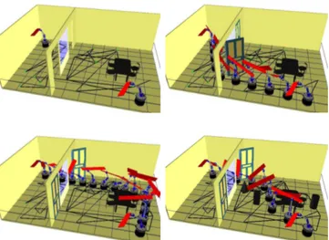
Fig. 1. Example of a 3D scene with moving obstacles: start and goal configurations of the 9dof mobile manipulator carrying a board and three path solutions obtained for several settings of the environment (doors closed/open and three other moving obstacles placed around the table)
This is mainly because the cost of reflecting dynamic changes into the roadmap during the queries is very high. On the other hand, single-query variants, which compute a new data structure for each new query, deal more efficiently with highly changing environments. They however do not keep the information reflecting the constraints imposed by the static part of the environment useful to speed up subsequent queries.
This paper aims at providing a practical planner that rapidly updates the roadmap at each query with only little preprocessing to account for obstacle changes. The planner combines several published ideas into an integrated solution allowing to answer queries very quickly when the moving obstacles have little impact on the free-space connectivity. As in [1], it uses lazy evaluation ideas to avoid spending too much time on updating the validity of roadmap edges that are not relevant to obtain the solution path. It also uses a single-query RRT planner [10] to rapidly check possible reconnections along some invalid edges of the roadmap. When the solution can not be found in the updated roadmap, the planner also integrates a reinforcement stage that possibly results into the creation of cycles representing alternative paths that were not yet stored in the roadmap.
gives an overview of the approach. Section III gives the details of the planner and explains how the queries are processed by lazily updating the roadmap connectivity and by reinforcing the roadmap when required. In section IV, we explain how this planner can be used for path-update and control of path execution. Finally, the performance of the planner is experimentally evaluated in Section V using several simulated environments.
II. PRESENTATION OF THE PROPOSED APPROACH A. Motivation
Let us consider a robot in an environment with static and moving obstacles. The problem consists of finding a collision-free path for this robot from an initial to a goal configuration, for specific positions of the moving obsta-cles. Figure 1 illustrates a typical example of such dynamic scenario. The robot (a 9dof mobile manipulator carrying a board) moves in an office-like environment. The moving obstacles in this example correspond to the two doors that are opened or closed and also to other moving objects located around the table (see the bottom/right image). They can invalidate part of the roadmap and we therefore need efficient mechanisms for updating this roadmap. The figure also shows for a same path query the different path solutions computed in real-time by the planner according to current context.
It is well known that PRM planners spend most of their time performing costly collision checks when constructing the roadmap. Several methods (e.g. [1], [15]) have been proposed for static environments to reduce the number of tests by postponing them as long as they are not really necessary.
In this paper, we apply a similar idea for planning in dynamic environments. In such dynamic context, we use the fact that moving obstacles often imply partial changes of the robot’s free space. Based on this remark, three main kind of methods are used to avoid collision tests:
• A lazy connection strategy is used to check
con-nections of the query nodes to the roadmap and to limit the update of the roadmap to portions which are relevant for obtaining the solution path.
• A local reconnection is attempted to reconnect edges temporary broken by mobile obstacles.
• An edge labeling mechanism stores previous positions of moving obstacles in the scene to relieve the number of collision tests for the edge.
These methods are detailed in section III.
B. General approach
Because the environment is only partially modified be-tween each of the queries, we use a two-stage method.
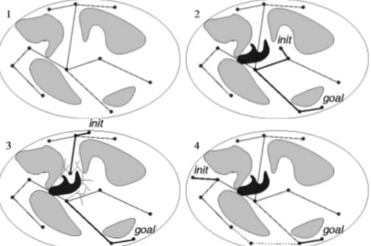
First, we compute a roadmap for the robot and the static obstacles, without considering the presence of the moving obstacles (Fig. 2.1). Then to solve the path query, portions of the roadmap are updated by checking if existing edges are collision-free with respect to the current position of the moving obstacles. Colliding edges are labeled as blocked in the roadmap. If this labeling permits to obtain a path which does not contain any blocked edge, then a solution is found (Fig. 2.2). When the solution path contains blocked
edges, a mechanism of local reconnection based on RRT techniques is used. It tries to reconnect the two extremities of those blocked edges (Fig. 2.3). Finally, if the existing roadmap does not allow to find a solution, new nodes are inserted and the roadmap is reinforced with cycle creation (Fig. 2.4). In practice, this general approach is combined with several methods avoiding unnecessary collision tests, which makes it more efficient. The next section presents the main features of the approach.
Fig. 2. A static roadmap is first computed in the configuration space of the robot (1). During queries, a solution path can be found directly inside this roadmap (2) or via a RRT like technique to reconnect edges broken by dynamic obstacles (3). If the existing roadmap does not permit to find a solution, new nodes are inserted and the roadmap is reinforced with cycle creation (4).
III. DETAILS OF THE APPROACH A. Roadmap labeling and solution path search
During path queries, the planner first checks whether a solution exists in the preprocessed roadmap. Hence, the roadmap edges already correspond to collision-free paths with respect to the static obstacles. They only need to be checked for collision with the moving obstacles. For efficiency reasons, it is useless to update edges which are not yet connected to the query nodes. Checking such direct connections with the query nodes is a costly operation since it also requires to check the edge validity with the static obstacles. It is therefore preferable to limit such tests a much as possible by avoiding systematic connections tests to all components of the roadmap after their dynamic update.
Based on the remarks above, the planner performs the roadmap labeling concurrently with the search for the solution path. It iteratively alternates the two following operations until a valid path is found or all connections have been attempted without success:
• Connection of query nodes to the nodes of the
roadmap.
• Search for a valid path inside the roadmap.
The search for a valid path yields the labeling of some edges in the roadmap. It first searches whether a statically valid path exists in the roadmap, and then updates the dynamic validity of the edges along the path. A solution is found when all edges remain collision-free with the moving
obstacles. Otherwise, the colliding edges are invalidated and used to reconstruct a part of the dynamic connectivity of the roadmap. The updated connectivity is then used at the next iteration to select the best candidate nodes in the roadmap in order to find other possible connections of the query nodes. We explain how these candidate nodes are selected based on the current connectivity information in the next paragraphs.
B. Query nodes connections
At each iteration, the candidate nodes are selected by decomposing each statically connected component into three sub-components : nodes potentially reachable from the init node, nodes potentially reachable from the goal node, and nodes which are currently not reachable from the query nodes. A roadmap’s node is potentially reachable from a query node if there exists a path linking both nodes, and which contains no blocked-labeled nodes.
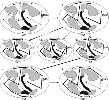
This selection mechanism is illustrated in Figure 3. The first selection is done considering that all roadmap nodes are not potentially reachable, and choosing among this set the closest node from each of the query nodes (Fig. 3.1). A statically valid path is then searched in the roadmap and the path edges labeled as blocked or valid in the dynamic context. The blocked edges (dashed edges of Fig. 3.2) modify the connectivity of the roadmap. The query connection extends the two sub-components of nodes reachable by the init and goal nodes while the blocked edges extend the third component gathering nodes which are not yet potentially reachable. The three sub-components are then used for the next selection. New connections are envisaged between the init (resp. goal) node and the set of nodes determined as reachable from the other query node (Fig. 3.3a-b) and also the connection to portions of the roadmap not yet connected to any query node (Fig. 3.3c). The next connection candidate in each set is selected as the closest node to the query one. The reason is that short local paths have a higher chance to be valid and collision detection along short paths is also more efficient. In this example, the third component (Fig. 3.3c) yields valid connections to both query nodes and the next path search/labeling (Fig. 3.4) yields the solution (Fig. 3.5).
In practice, this method avoids many costly updates of edges that are not strictly necessary to answer the query. In particular, the components of the roadmap which are not connected to the query nodes will never be tested.
C. Local reconnections
As explained above, for each new connection of the query nodes to the roadmap, the algorithm tries to find a solution path which does not contain blocked edges. If such a path cannot be directly extracted from the roadmap, the algorithm tries to solve the problem locally, using a Rapidly exploring Random Tree planner to connect the endpoints of the blocked edges. The principle of the bidirectional
RRT-Connect algorithm (see [10]) used in our reconnection
planner consists of incrementally building two random trees rooted at the start and goal configurations. The complexity of RRT depends on the length of the solution path. This means that the approach quickly finds easy
Fig. 3. Query nodes are connected to the roadmap (1) and a first attempt to find a valid path is done. If this attempt fails, it means that some edges have been labeled as blocked (2). Then three new connections are envisaged : connection of a query node to nodes potentially reachable from the other query node (3.a, 3.b) and connection to portions of the roadmap no more connected to any query node (3.c). In this exemple, the last kind of connection (4) permits to find a valid path (5).
solutions. If the mechanism of broken edges reconnection fails, a new connection from the query nodes to the static roadmap is attempted as described in Sect. III.B.
D. Nodes insertion and cycles creation
If all connections have been attempted without success, new nodes are added to the roadmap to solve the query. These nodes are connected to the different components of the roadmap taking into account the partial edge labeling previously achieved. Such new nodes are necessary to find an alternative way to dynamically re-connect disjoint com-ponents that were previously linked in the static roadmap (see Fig. 2.4). Because this reinforcement stage only occurs when local reconnections have failed, we avoid the creation of needless edges and nodes inside the roadmap which could reduce the efficiency of the planner for future queries.
E. Edge labeling
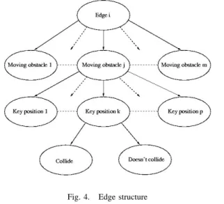
The planner uses the information gained during the queries to increase the efficiency of the edge labeling process. This allows to reduce the cost of the queries. For this, a specific data structure is added to the roadmap (figure 4).
This structure stores information for key positions of moving obstacles. When the Edge-Labeling function is called, current positions of moving obstacles are compared to positions already stored and information derived from previous collisions checks is reused (see Algorithm 1).
The first time the Edge-Labeling function is called for a given edge E, no specific information has been stored so far. Collisions tests are done classically, until a collision is detected or all the moving obstacles are tested. Concurrently, results of all those tests are stored in the data structure, taking the current positions of each moving
Fig. 4. Edge structure
Algorithm 1 Edge-Labeling(E) for each Movable Obstacle M Oi do
for each Key Position KPj of M Oi stored in E do if KPj = Current Pos then
is-collision←Extract-Col-Info(E,KPj) else
is-collision←Col-test(E, MOi)
Store is-collision in R
end if
if is-collision = TRUE then
Return invalid
end if end for end for
Return valid
obstacles as key positions. The next time the Edge-Labeling function is called for this edge, the current position of
M Oi is compared to the stored positions. If one of the
stored positions is the same as the current one, the result of the previous collision test is extracted and the new test is avoided (Extract-Col-Info of algorithm 1). Otherwise, the new position is inserted in the edge structure. This principle is repeated for all the calls of the Edge-Labeling function. Because obstacles can continuously move in the environment, leading to an infinity of intermediate positions, we only keep the last checked positions. Older positions are removed from the data structure in order to limit the size expansion of the roadmap. In practice, the memorization of the information concerning only the few last positions is sufficient to avoid many useless tests as in the two following kind of situations : when a moving obstacle has discrete positions (e.g. doors which can be open or closed), it is only considered for collisions the first time it is placed at one of the discrete positions. Also when a moving obstacle stops (e.g. displaced object, stopped robot), it starts to be treated exactly as static objects and unnecessary collision tests are avoided.In summary, the only collision tests which are needed to be performed for a given edge, are the ones that correspond to new positions of moving obstacles.
IV. PATH UPDATE AND CONTROL OF PATH EXECUTION
The dynamic planner has also been tested in applications requiring real-time performance. Two kinds of problems have been addressed for environments with continuous changes :
• Update of a valid path. • Control of a path execution.
The mechanism used is very similar in both cases. For path update, a valid path is first computed as explained above. Then, its validity is checked at different time steps with some moving obstacles. When the path collides, a local reconnection mechanism, as proposed for the edges of the roadmap is attempted. If it fails, our planner finds a new path, valid in the current context. During path execution, in addition to path update, the robot goes forward along the path for a fixed length if the update has succeeded. In practice we only test the portions of the path the robot will cover soon. This avoids changing the solution when an obstacle crosses the path far from the actual robot position and may have disappeared when the robot arrives there. In section V-E, we show an example using these mechanisms.
V. EXPERIMENTALRESULTS
The dynamic planner was implemented within the soft-ware platform Move3D [17] developed at LAAS. The reported computation times correspond to experiments con-ducted on a 333 MHz Sun Blade 100 workstation. Each value given in the tables has been averaged over 20 runs of the planner. Indicated collision tests correspond to the sum of the static and dynamic collisions tests performed.
A. Global Performance
The first experiment compares our planner with two other planners : the single-query planner bi-RRT [10], and a planner based on a roadmap precomputed with a
visibility-PRM method [16]. The later one uses a systematic update
of the validity of all the roadmap edges (called “global la-beling”) instead of the lazy connection strategy performed by the dynamic planner. The environment used for the test is the office-like scene shown in figure 1. It contains two doors which are randomly closed or opened before each query and also three other moving objects randomly placed around the table. Comparative performance results are shown in table I.
bi-RRT Visibility Dynamic PRM Planner Time (s) 4.3 1.1 0.2 Collisions 5697 1722 356 Edges 45 78 78 Tested edges 45 78 18 TABLE I
PERFORMANCE OF THE DYNAMIC PLANNER COMPARATIVELY TO TWO OTHER PLANNERS.
One can note that the “global labeling” method is more efficient than the single query one. Even if more edges are tested (78 against 45), they are only checked for collisions against moving obstacles, which significantly decreases the
overall cost of collision checking. One can also note the gain of the lazy connection and edge labeling mechanisms used by the dynamic planner compared to a systematic labeling. The number of collision tests is almost divided by 5, even for the small size of roadmaps computed for this example.
Fig. 5. An example of query (left) and the path solution (right), in an environment with static columns and 20 cube-shaped moving obstacles.
B. Lazy labeling
To further evaluate the performance of the lazy connec-tion strategy, we performed tests on the environment of figure 5 for several sizes of the precomputed roadmaps (containing or not cycles), and also for a different number of moving obstacles. The different settings are summarized in the table below:
Test Mov. obstacles Nodes Edges
A 5 100 99
B 5 100 318
C 20 100 99
D 20 100 318
E 20 200 700
The environment is composed of 13 static columns and several cube-shaped moving obstacles. The robot is the same 9dof mobile manipulator used in the previous environment. Both, the query nodes and the positions of the moving obstacles are randomly chosen. Because we analyze here the edge labeling, solutions involving addition of new nodes are not retained for results. Table II presents the results of the tests.
A B C D E Lazy connection Time (s) 0.2 0.3 0.7 1.0 1.7 Collisions 340 478 640 681 1379 % of tested edges 9.1 4.1 10.1 5.7 6.1 Global labeling Time (s) 2.4 3.6 4.8 7.3 15.7 Collisions 4602 7123 4882 6809 14338 % of tested edges 100 100 100 100 100 TABLE II
INFLUENCE OF THE LAZY CONNECTION ACCORDING TO THE NUMBER OF MOVING OBSTACLES AND THE ROADMAP SIZE.
The techniques using lazy labeling are from 7 to 12 times faster than a global edge labeling. This can be explained by the small fraction of the roadmap explored.
C. Edge labeling
The environment of figure 5 is also used to analyze the efficiency of the edge labeling mechanism. The roadmap
Fig. 6. Creation of roadmap cycles for a 3dof robot (top) evolving in a virtual house. A first roadmap is computed without taking into account doors (left). Then, after several queries, roadmap is reinforced with new cycles (right). Dashed edges correspond to edges invalid in the current context.
and the moving obstacles are the same as described in the test D. Figure 7 shows the average time to label edges of the roadmap, depending of the number of moving obstacles whose position is stored in the roadmap structure.
Fig. 7. Influence of edge labeling: computation time decreases with the number of stored positions
As we would expect, the time for edge labeling decreases linearly with the number of positions stored in the roadmap. For the extremal case where all the current positions of moving obstacles are stored in the roadmap, no collision test is done when checking the validity of the edges.
D. Cycles creation
Figure 6 shows the house environment used to illustrate the mechanism of cycle creation. It contains many static obstacles which represent a total geometrical complexity of 70000 facets and 7 doors used as moving obstacles that are opened or closed. The robot used is the 3dof
mobile robot shown in the top image. The bottom left image shows the “static” roadmap that was first computed using the Visibility-PRM technique [16], without consid-ering the doors. In the example, it permits to capture the connectivity of the free space with only 33 nodes. Then, ten queries were solved by the planner for randomly chosen open/closed positions of each door. When the solution can not be found within the current roadmap, nodes are inserted with the Visibility-PRM technique. The bottom right image shows that after the queries, the roadmap is reinforced with 3 nodes and 11 edges creating several useful cycles. In total, 3.5 seconds were spent for the roadmap reinforcement during the ten queries (i.e. an average of .35 sec. per query).
E. Real-time applications
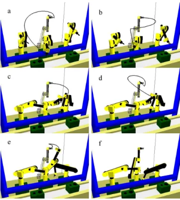
Figure 8 shows an example of path execution controlled by the dynamic planner. The robot is a 6dof manipulator arm in an assembly line environment. It is surrounded by two other articulated arms considered as moving obstacles. The first image shows the start and goal configurations of the problem (the goal is wireframed) and the trajectory initially computed. The planned trajectory is executed, but it is successively perturbed by the motions of the two other arms of the assembly line. Then, it is dynamically updated with our planner during its execution.
Fig. 8. Trajectory execution controlled by the dynamic planner for a 6dof manipulator arm in an assembly line environment.
This example illustrates the capability of the planner to work with real time performances. Several movies illustrating real-time path updates and control of path execution are also available onhttp://www.laas.fr/ ~ljaillet.
VI. CONCLUSION AND PERSPECTIVES
In this paper we proposed a roadmap planner designed to operate in dynamically changing environments. The plan-ner relies on several lazy evaluation mechanisms allowing a partial but fast dynamic update of the roadmap to answer path queries as fast as possible. Preliminary experiments are promising. They show the capability of the planner to solve real-time problems in geometrically complex scenes with several moving obstacles. Several improvements re-main for future work. In particular it should be further investigated how to relate workspace changes to particular regions of the roadmap that can be potentially affected, in order to further limit the validity tests to the relevant portions of the roadmap.
ACKNOWLEDGMENT
This work has been supported by the European project IST-2001-39250 MOVIE.
REFERENCES
[1] R. Bohlin, L. Kavraki. “Path Planning Using Lazy PRM”. In Proc.
of the Int. Conf. on Robotics and Automation, 2000.
[2] O. Brock, L. Kavraki. “Decomposition-based Motion Planning: A Framework for Real-time Motion Planning in High-dimensional Configuration Spaces”. In IEEE Int. Conf. on Robotics and
Automa-tion, 2001.
[3] O. Brock and O. Khatib. “Elastic Strips: A Framework for Integrated Planning and Execution”. In Proc. Int. Symp. on Experimental
Robotics, 1999.
[4] O. Brock, O.Khatib. “Real time replanning in high-dimensional configuration spaces using sets of homotopic paths”. In Proc. IEEE
Int. Conf. on Robotics and Automation, 2000.
[5] M. Cherif, M. Vidal. “Planning handling operations in changing industrial plants”. In Procs of the IEEE on Robotics and Automation, 1998.
[6] E. Feron, E. Frazzoli and M. Dahleh. “Real-time motion planning for agile autonomous vehicles”. In AIAA Conf. on Guidance, Navigation and Control, Denver, August 2000.
[7] D. Hsu, R. Kindel, J.C. Latombe, S. Rock. “Randomized Kino-dynamic Motion Planning with Moving Obstacles”. In Proc. of
the Workshop on Algorithmic Foundations of Robotics (WAFR’00),
2000.
[8] D. Hsu, J.C. Latombe, R. Motwani. “Path planning in Expansive Configuration Spaces”. In Proc. of the IEEE Int. Conf. on Robotics
and Automation, 1997.
[9] L. Kavraki, P. Svestka, J.-C. Latombe, and M. OverMars. “Proba-bilistic Roadmaps for Path Planning in High-Dimensional Config-uration Spaces”. In IEEE Transactions on Robotics and
Automa-tion,12(4), 1996.
[10] J. Kuffner, S.LaValle. “RRT-Connect: An efficient Approach to Single Query Path Planning”. In Proc. of the IEEE Int. Conf. on
Robotics and Automation, 2000.
[11] J.C. Latombe. “Robot motion planning”. In Kluwer academic Press, 1991.
[12] P. Leven S. Hutchinson “Toward Real-Time Path Planning in Changing Environments”. In Proc. of the Workshop on Algorithmic
Foundations of Robotics, 2000.
[13] A. McLean, I. Mazon. “Incremental Roadmaps and Global path Planning in Evolving Industrial Environments”. In Proc. of the IEEE
Int. Conf. on Robotics and Automation, 1996.
[14] M.H. Overmars “Algorithms for motion and navigation in virtual environments and games”. In Proc. of the Workshop on Algorithmic
Foundations of Robotics, 2002.
[15] G. Sanchez, J.C. Latombe, “A Single Query Bi-Directional Prob-abilistic Roadmap Planner with Lazy Collision Checking”. In
International Symposium on Robotics Research, Lorne, Victoria,
Australia, November 2001.
[16] T. Siméon, J.P. Laumond, C. Nissoux. “Visibility based Probabilistic Roadmaps for Motion Planning”. In Advanced Robotics Journal, 14(6), 2000.
[17] T. Siméon, J.P. Laumond, C. van Geem and J. Cortés. “Computer Aided Motion: Move3D within MOLOG.”. In IEEE Int. Conf. on