IMPROVED CONDITIONING TO HARD, SOFT AND DYNAMIC DATA IN MULTIPLE-POINT GEOSTATISTICAL SIMULATION
HASSAN REZAEE
DÉPARTEMENT DES GÉNIES CIVIL, GÉOLOGIQUE ET DES MINES ÉCOLE POLYTECHNIQUE DE MONTRÉAL
THÈSE PRÉSENTÉE EN VUE DE L’OBTENTION DU DIPLÔME DE PHILOSOPHIÆ DOCTOR
(GÉNIE MINÉRAL) MAI 2017
c
ÉCOLE POLYTECHNIQUE DE MONTRÉAL
Cette thèse intitulée :
IMPROVED CONDITIONING TO HARD, SOFT AND DYNAMIC DATA IN MULTIPLE-POINT GEOSTATISTICAL SIMULATION
présentée par : REZAEE Hassan
en vue de l’obtention du diplôme de : Philosophiæ Doctor a été dûment acceptée par le jury d’examen constitué de :
M. GOULET James, D.Sc., président
M. MARCOTTE Denis, Ph. D., membre et directeur de recherche M. ORTIZ Julian, Ph. D., membre
DEDICATION
ACKNOWLEDGMENTS
I would like to express my sincere thanks to Prof. Denis Marcotte for accepting me, funding my studies, and his constant support during four years. That was always a push to try harder for the perfection and completion of the work. It was quite frightening on the first place to come to Canada’s cold from Iran ! Denis was very responsive throughout the years and extremely supportive.
I use the opportunity to thank my kind parents and siblings. I’m grateful beyond words. This PhD was quite an adventure in its kind, by far the best PhD I have ever done ! It made possible due to the support of Denis in the first place and second all the wonderful people I came to meet during the internships.
My first internship with CGG Crawley, UK, was a great opportunity to see how industry handles problems related to geological modelling in real studies. In particular I thank Philippe Doyen, Thierry, Salman, Théophile, Rémi and the other Rémi !
The second internship with Jason CGG in The Hague, Netherlands, was a perfect entry point to field of geophysical seismic data processing and inversion, cheese tasting and Heineken ! I would like to thank Ali Moradi Tehrani, Raphael Bornard, Reza Saberi, Sarah Boudon and Mengmeng Zhang. The tests on seismic inversion gave us a better understanding in the case study of Chapter 4 on soft data conditioning.
I also would like to thank Pierre Biver, Tatiana Chugunova and Florent Piriac whose support for the third internship with TOTAL S.A. Pau, France, provided me a great opportunity for hands-on experience in reservoir geological modelling, and wine tasting ! It will always be an asset to me the internship with TOTAL.
All my friends, in Montreal, Europe and Iran that I happened to meet, work and hang out with during PhD and internships ; I appreciate their company and the time we spent together. In particular I would like to thank Yahya, Mohammad, Ali and Amir.
In the end, I would like to thank my dear friends, Jafar, Alireza, Abbas, Reza and Morteza from Zenjkadeh group at University of Tehran.
RÉSUMÉ
Dans cette dissertation, nous présentons trois méthodes visant à corriger autant de problèmes observés dans les simulations géostatistiques basées sur des statistiques multipoint (MPS). Le premier problème est le conditionnement aux données exactes (hard data) des algorithmes MPS par morceaux (patch-based). Le second problème est l’utilisation efficace de données auxiliaires (soft data) dans le MPS. Le dernier problème est la calibration des réalisations de faciès par MPS à des données dynamiques. Bien que le premier problème soit particulier au MPS par morceaux les deux autres sont communs à toutes les variantes de MPS ainsi qu’aux autres méthodes de modélisation des faciès.
Dans une simulation MPS de variables catégoriques les données exactes trouvées dans le voisinage de recherche du point à simuler souvent ne correspondent à aucun des patrons disponibles dans l’image d’entrainement (TI). La solution habituellement utilisée est alors d’ignorer les points du voisinage les plus éloignés jusqu’à ce que le patron soit retrouvé dans la TI. Nous proposons plutôt l’utilisation de TI alternatives (ATI) permettant d’enrichir la base de données des patrons. Les ATIs sont obtenues par simulation non-conditionnelle (MPS par morceaux) à partir de la TI originale (OTI). Parmi toutes les ATI générées, certaines seulement sont sélectionnées en fonction des structures observées et des statistiques présentes dans ces ATI par rapport aux statistiques et aux structures des OTI. On vérifie également que chaque ATI apporte suffisamment de patrons présents dans les données exactes observées. Les ATIs qui ne sont pas assez riches en patrons observés ou qui ne sont pas statistiquement similaires à l’OTI, ou qui ont un contenu structurel différent de l’OTI sont rejetées. Les ATIs sélectionnées et l’OTI sont ensuite transmises à la boucle principale de simulation. Le nombre et la taille des ATIs sélectionnées peuvent être aussi grands que souhaité pourvu que les temps de calcul demeurent réalistes. Nous avons testé l’approche sur plusieurs TI différentes, catégoriques et continues, en 2D et en 3D. Nos résultats montrent que l’utilisation des ATIs améliore le conditionnement aux données exactes, améliore la reproduction de la texture des TI et permet de simuler sur de grandes grilles même à partir de petites OTI.
Le conditionnement des modèles de faciès à des données auxiliaires est complexe, en rai-son de relations mal connues, souvent non-linéaires, liant les faciès et les données auxiliaires continues. Dans cette étude, nous proposons de calculer des champs de probabilité à partir des données auxiliaires en utilisant la régression logistique multinomiale. La méthode permet d’intégrer plusieurs variables auxiliaires correspondant par exemple à autant de méthodes géophysiques. Elles sont exploitées avec les données exactes pour estimer par régression lo-gistique multinomiale les champs de probabilités de chaque faciès. Plus la relation entre les
données exactes et auxiliaires est forte, plus les champs de probabilité obtenus sont informa-tifs. Les champs de probabilité sont ensuite transférés à la boucle principale de simulation MPS. Pour chaque morceau à simuler, la sélection sur l’OTI ou les ATI se fait à l’aide d’une distance constituée de deux termes. Un premier terme mesure la reproduction des données exactes et la continuité de la texture, un second terme compare les proportions de chaque fa-cies dans le morceau aux probabilités dans la zone à simuler. Ces deux termes sont combinés avec un poids défini par la qualité de la régression logistique. La méthode a été testée sur différents exemples synthétiques avec et sans données exactes et avec des variables auxiliaires présentant des degrés variables de corrélation avec les données exactes. Une étude de cas du champ d’hydrates de gaz de Mackenzie a été réalisée. Les teneurs dans les puits ont été uti-lisées comme données exactes. L’image tomographique de la teneur du gaz entre deux puits a été utilisée comme TI 2D et les données d’impédance acoustique provenant de l’inversion sismique ont servi de données auxiliaires. Des réalisations multiples obtenues avec l’approche proposée ont montré une bonne correspondance entre la carte d’espérance des réalisations (e-type) et les probabilités calculées.
Le problème de la calibration des modèles de faciès à des données dynamiques (e.g. des flux) est plus difficile que la calibration à des données statiques puisque par exemple la relation entre l’arrangement spatial des faciès et la réponse des flux peut être très complexe. La première étape de l’approche proposée consiste à obtenir des réalisations MPS conditionnelles aux données exactes et auxiliaires. Dans une seconde étape les réalisations de faciès sont converties en champs gaussiens grâce à une règle de codage et un simulateur de Gibbs, tout comme avec la méthode de simulation plurigaussienne. Dans une troisième étape, les champs gaussiens sont perturbés par déformation graduelle (GDM) afin de s’approcher des données dynamiques observées. Le GDM a été intégré à un processus évolutif s’inspirant d’algorithme génétique. Une population est formée et évolue au fil des générations qui se succèdent. Chaque génération comporte un mélange de réalisations évoluées obtenues par GDM et de réalisations directement issues du MPS, ces dernières assurant le maintien de suffisamment de diversité génétique au sein de la population. Les générations se suivent jusqu’à ce que les critères d’arrêt soient respectés. L’algorithme proposé est général et peut s’appliquer à toute méthode de simulation de faciès. Il a été testé sur plusieurs cas 2D et 3D avec différents types de données dynamiques. Dans tous les cas, la calibration aux données dynamiques a été grandement améliorée par rapport aux résultats obtenus avec les MPS non-calibrés.
Les idées proposées pour le conditionnement et la calibration des modèles MPS ont été ras-semblées en un test intégré. L’exemple comprenait une TI 2D, 250 données exactes, trois variables auxiliaires, et trois puits avec des données dynamiques de production. Les données
auxiliaires ont été utilisées dans la régression logistique multinomiale pour calculer les cartes de probabilité. Plusieurs réalisations MPS ont été générées conditionnellement aux données exactes et auxiliaires et ont été utilisées pour générer des champs Gaussiens en utilisant l’échantillonnage de Gibbs. L’approche GDM-évolutionnaire a été appliquée pour la calibra-tion des modèles aux courbes pétrole/eau. Le GDM-évolucalibra-tionnaire s’est avéré efficace pour calibrer ces modèles aux données dynamiques. Les résultats montrent l’importance de bien intégrer les données auxiliaires et dynamiques dans les réalisations MPS.
Les stratégies de conditionnement des MPS présentées dans cette dissertation forment un tout cohérent et intégré permettant la production de modèles de faciès de haute qualité (texture) respectant les données exactes, auxiliaires et dynamiques obtenues de sources diverses. Ces modèles améliorés de faciès constituent un élément essentiel pour une meilleure prévision des performances des réservoirs et gisements et fournissent un outil permettant de guider les décisions stratégiques d’exploitation des ressources et d’évaluer l’incertitude associée. La dissertation se termine sur quelques suggestions pour travaux futurs.
ABSTRACT
In this dissertation, we present three methodologies to correct three problems observed in geostatistical simulations based on multiple-point statistics or MPS. The first problem is the conditioning to hard data of patch-based algorithms. The second problem is the efficient use of auxiliary data in patch-based MPS. The last is the calibration of facies realizations to dynamic data. The first problem is particular to patch-based MPS while the second and third are common between not only MPS approaches but also other facies modeling methods. In an MPS simulation of categorical variables, hard data found within the search neighbour-hood of simulation point often do not match exactly any of the patterns available in TI. One common solution to this problem is to drop out farther nodes until a matching pattern is found in TI. We propose instead using Alternative TIs (ATI) to enrich the pattern database. ATIs are mainly unconditional patch-based simulations based on original TI (OTI). Among the ATIs generated, some are selected based on the structures observed and their statistical features (histogram and variogram) compared with those of OTI. Their pattern databases are examined for the frequency of matching patterns with existing hard data configurations in simulation grid. ATIs that are not rich enough (as measured by number of matches for the hard data), not statistically similar to OTI, or with different structural content from OTI are discarded. The selected ATIs and OTI then are passed onto the main simulation loop. ATIs can be considered of any size and number as long as they are not computationally prohibitive for MPS simulation. We have tested the idea over several 2D and 3D TIs for categorical and continuous variables. Our test results show that using ATIs enhances the conditioning capa-bilities, improves the texture reproduction, and allows simulating over large grids even using much smaller OTIs.
The conditioning of facies models to soft data is complex due to the imperfectly known non-linear relationship between categorical facies types and continuous soft data. In this study we propose calculating probability maps from soft data using multinomial logistic regression. This method allows integrating multiple soft data layers, namely different geophysical data sets. All soft data layers are exploited simultaneously in conjunction with hard data to calculate the facies probability maps. The stronger is the relationship between hard and soft data, the more informative are the output probability maps. The probability maps are then transferred to the main MPS simulation loop. At each patch under simulation, the selection of OTI or the ATIs is performed using a two-term distance function. The first term measures the reproduction of hard data and the continuity of texture, and the second term compares the proportion of each facies in the patch with the probability maps. These
components are merged using a weight determined by the quality of logistic regression. The method was tested over different synthetic examples with and without hard conditioning data and over varying degrees of correlation between hard and soft data. A case study of the Mackenzie gas hydrate field was performed. Grade data sampled on the wells were used as hard data. The tomography image of gas grade between two wells was taken as 2D TI, and the acoustic impedance data from seismic inversion as soft data. Multiple realizations using the proposed approach showed a good match between e-type map of realizations and the calculated probabilities maps.
The problem of calibration of facies models to dynamic data (e.g., flow data) is more diffi-cult than the static soft data since the relationship between facies arrangement and the flow response can be very complex. The first step of the proposed approach consists of obtaining conditional MPS realizations to hard and soft data. In a second step the facies realizations are converted into Gaussian fields using the lithotype rule, and Gibbs Sampling method, all similar to the PluriGaussian simulation method. In a third step, the Gaussian fields are per-turbed using the Gradual Deformation Method (GDM) in order to calibrate to the observed dynamic data. The GDM was modified resembling a Genetic Algorithm evolutionary process. A population of perturbed models is formed and evolves over successive generations. Each generation comprises a mixture of perturbed realizations obtained by GDM and realizations directly derived from MPS, the latter ensuring the maintenance of sufficient genetic diversity within the population. The generations evolve until a stopping criteria is met. The proposed algorithm is general and can be applied to all facies simulation methods. It was tested over several 2D and 3D cases with different types of dynamic data. In all cases, the calibration to dynamic data was largely improved compared with non-calibrated MPS realizations. The proposed ideas for conditioning and calibration of MPS models were put together in an integrated test. The example included a 2D TI, 250 hard data, three soft data variables, and three production wells with dynamic data. The soft data layers were used in multino-mial logistic regression to calculate the probability maps. Multiple MPS realizations were generated conditioned to hard and soft data and were used to generate Gaussian fields using Gibbs Sampling. The proposed evolutionary GDM was applied on the realizations for the calibration of models to water cut curves. The evolutionary GDM has proven to be effec-tive in calibrating the facies models to dynamic data. The results show the importance of integrating the auxiliary and dynamic data into the MPS realizations.
The conditioning strategies of MPS presented in this dissertation form a coherent and inte-grated set of tools allowing the production of facies models of high quality (texture) respecting the hard, auxiliary and dynamic data obtained from various sources. These improved facies models are an essential element for better prediction of reservoir and deposits performance
and provide a tool to guide strategic resource decisions and assess the associated uncertainty. The dissertation ends with some suggestions for future work.
TABLE OF CONTENTS DEDICATION . . . iii ACKNOWLEDGMENTS . . . iv RÉSUMÉ . . . v ABSTRACT . . . viii TABLE OF CONTENTS . . . xi LIST OF TABLES . . . xv
LIST OF FIGURES . . . xvi
LIST OF INITIALS AND ABBREVIATIONS . . . xxv
CHAPTER 1 INTRODUCTION . . . 1
1.1 Facies Modeling . . . 1
1.2 Why Using MPS ? . . . 2
1.3 MPS Workflow . . . 4
1.4 Patch-based MPS . . . 5
1.5 Potential problems with patch-based MPS . . . 6
CHAPTER 2 PROBLEM STATEMENT AND LITERATURE REVIEW . . . 10
2.1 Elements of the Problem . . . 10
2.1.1 Hard Data Conditioning . . . 10
2.1.2 Soft Data Conditioning . . . 13
2.1.3 Dynamic Data Conditioning . . . 23
2.2 Objectives of the Research . . . 27
2.2.1 General objective . . . 27
2.2.2 Specific objectives . . . 27
2.3 Plan of the Thesis . . . 28
CHAPTER 3 ARTICLE 1: MULTIPLE-POINT GEOSTATISTICAL SIMULATION USING ENRICHED PATTERN DATABASES . . . 29
3.2 Introduction . . . 30
3.3 Methodology . . . 31
3.3.1 Weighting system . . . 33
3.3.2 Pasting . . . 33
3.3.3 Flowchart . . . 38
3.3.4 Alternative Training Images . . . 38
3.3.5 ATI selection strategy for the categorical and the continuous cases . . 44
3.4 Results . . . 49 3.4.1 Continuous TI . . . 50 3.4.2 Categorical TI . . . 54 3.4.3 3D simulations . . . 58 3.4.4 CPU Time . . . 61 3.5 Discussion . . . 61 3.6 Conclusion . . . 66 3.7 Acknowledgements . . . 67
CHAPTER 4 ARTICLE 2: INTEGRATION OF MULTIPLE SOFT DATA SETS IN MPS THRU MULTINOMIAL LOGISTIC REGRESSION: A CASE STUDY OF GAS HYDRATES . . . 68
4.1 Abstract . . . 68
4.2 Introduction . . . 69
4.3 Methodology . . . 71
4.3.1 Getting the probability fields . . . 71
4.3.2 Simulating using MPS . . . 72
4.3.3 Influence of the logistic regression . . . 76
4.4 Simulation Results . . . 76
4.4.1 Multiple soft data sets . . . 79
4.4.2 3D simulations . . . 82
4.4.3 Sensitivity to α . . . . 82
4.5 Hard Data conditioning . . . 82
4.5.1 Regional effect of HD locations . . . 88
4.6 Real TI and Soft Data Conditioning . . . 88
4.7 Discussion . . . 98
4.8 Conclusions . . . 98
4.9 Acknowledgement . . . 98 CHAPTER 5 ARTICLE 3: CALIBRATION OF CATEGORICAL SIMULATIONS BY
EVOLUTIONARY GRADUAL DEFORMATION METHOD . . . 100
5.1 Abstract . . . 100
5.2 Introduction . . . 101
5.3 Methodology . . . 102
5.3.1 MPS method . . . 103
5.3.2 Latent Gaussian variables . . . 103
5.3.3 Deformation in Gaussian space . . . 105
5.3.4 Facies noise removal . . . 107
5.3.5 Optimization . . . 109
5.4 Results . . . 110
5.4.1 Proportion map example . . . 110
5.4.2 Shortest path 2D example . . . 112
5.4.3 Seismic section example . . . 112
5.4.4 Shortest path 3D example . . . 117
5.4.5 Water Cut Example, 2D Case . . . 117
5.4.6 Water Cut Example, 3D Case . . . 117
5.5 Discussion . . . 122
5.6 Conclusions . . . 126
5.7 Acknowledgement . . . 126
CHAPTER 6 INTEGRATED MODEL . . . 127
6.1 Introduction . . . 127 6.2 Input data . . . 127 6.2.1 Probability maps . . . 129 6.2.2 Dynamic data . . . 131 6.3 Modelling Process . . . 133 6.3.1 TI Enrichment . . . 133
6.3.2 Hard Data Conditioned Models . . . 134
6.3.3 Soft Data Conditioned Models . . . 136
6.3.4 Hard and Soft Data Conditioned Models . . . 137
6.3.5 Global dynamic behaviour of conditioned models . . . 139
6.3.6 Calibrated Models . . . 140
6.4 Discussion and Conclusions . . . 147
CHAPTER 7 DISCUSSION AND CONCLUSION . . . 148
7.1 Discussion . . . 148
7.3 Conclusions . . . 152 REFERENCES . . . 154
LIST OF TABLES
Table 3.1 Distribution of patterns found in OTI and ATI . . . 46 Table 5.1 Parameters used in the 2D and 3D water cut examples. . . 118
LIST OF FIGURES
Figure 1.1 The significant difference between the flow response of channels simula-ted with SISIM and MPS. The facies models on left column are colored with permeability values. The right column shows the travel time (in logarithmic scale) between source and sink. . . 3 Figure 1.2 The basic idea behind MPS simulation. . . 5 Figure 1.3 Patch-based vs. pixel-based MPS simulation. . . 6 Figure 1.4 Pixel-based vs. patch-based approaches in generating texture.
Simula-tion using T=22 and OL=21 is a pixel-based simulaSimula-tion since the size of patch is reduced to only one pixel. Simulations are performed using distance-based approach based on quilting and a unilateral simulation path. . . 7 Figure 1.5 Patch-based MPS simulation using distance functions. It is not
neces-sarily the pattern in TI corresponding to minimum distance that is selected, but instead a pool of pattern is first formed from the lowest distance values, and one pattern is picked at random and pasted to the simulation grid. The red plus sign shows the upper left corner loca-tion of the selected pattern and three white dots on the distance map indicate other three corners. . . 8 Figure 2.1 The recursive template splitting idea as used in CCSIM (Tahmasebi
et al, 2012). The original template with overlap regions in gray and the parts to be simulated in green are highlighted in the simulation grid on left. Right column shows the process through which the original template is split recursively until the matching pattern is found in TI. 12 Figure 2.2 Top: three selected TIs, bottom-left: probability of finding a perfect
matching pattern from the TI vs. data event size, bottom-right: por-tion of the original data event that has to be droped out until we find a matching pattern in the TI. . . 14 Figure 2.3 Same test as in Fig. 2.2 repeated with and without ATIs. The
proba-bility of finding a matching pattern on left columns and the portion of original data event dropped out to find a matching pattern as a func-tion of data event size for channel TI (A), dunes TI (B) and multi-facies channel TI (C), see Fig. 2.2. . . 15
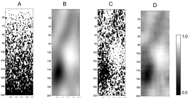
Figure 2.4 The TI, rotation map and the proportion maps were used to perform conditional simulations. Sample simulations are presented with dif-ferent Tau values. With permission from Liu (2006). . . 17 Figure 2.5 A: TI, B: auxiliary variable, C: sample simulation and D: e-type map
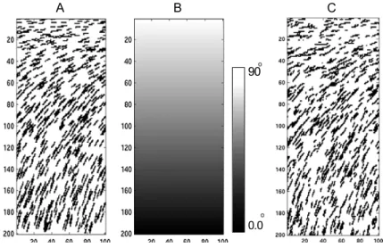
of 50 realizations. With permission from Chugunova and Hu (2008). . 18 Figure 2.6 A: TI, B: auxiliary variable, C: sample simulation. With permission
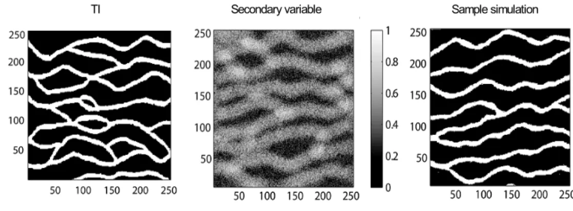
from Chugunova and Hu (2008). . . 19 Figure 2.7 Sample conditional simulation of the method proposed with Mariethoz
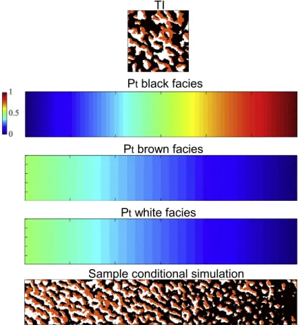
et al (2010). The TI (left) has been used to perform the conditional simulation (right) using the soft data on middle. With permission from Mariethoz et al (2010). . . 21 Figure 2.8 Sample conditional simulation of the method proposed with Mariethoz
et al (2015). The TI on top has been used to perform the conditional simulation shown on bottom using the proportion maps of different facies in the middle rows. With permission from Mariethoz et al (2015). 22 Figure 3.1 Schematic illustration of a patch in (A) unilateral and (B) random
simulation paths. Gray pixels are already simulated, white ones are to simulate, and black pixels represent HD. The irregular shape of B is due to random selection of previous patch centroids. . . 34 Figure 3.2 Enlarged window to include nearby conditioning data in the distance
computations. Only the hatched area in the initial window is pasted with data from the matching pattern in the OTI or ATI. . . 35 Figure 3.3 Weighting sets for HD (a1) and previously-simulated parts (a2) and
the final weighting matrix (α). In this case, the node highlighted in bold red square receives the highest weight. The illustration shows the weighting system for the L-shaped patch (for other possible patches see Fig. 3.4) . . . 36 Figure 3.4 Patch shapes and the corresponding weighting system. Left: first row,
middle: first column, and right: the rest of the image. W stands for the weight given to each band in the template. . . 37 Figure 3.5 Three possible stitching strategies in simulation. A: new pattern is
pla-ced without overlap, B: the overlap is overwritten by the new pattern, C: the overlap is cut through the minimum error path . . . 39 Figure 3.6 P 1 is the new pattern coming from either OTI or ATI, and P 2 is the
existing pattern simulated before. P 1 and P 2 are stitched along the series of pixels where the minimum overlap error is achieved (decoupage) 40
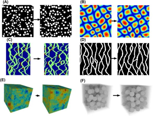
Figure 3.7 Quilting in a 3D parallepiped with multiple surface cuts. . . 41 Figure 3.8 The flowchart of the algorithm . . . 42 Figure 3.9 Sample OTIs (left) with corresponding ATIs (right) obtained by
uni-lateral unconditional simulation with weighting and decoupage. . . . 43 Figure 3.10 MPH computed over 4 × 4 templates; X: first eigenvector (18 %
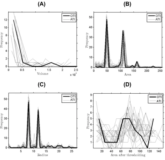
of variance), Y: second eigenvector (13%) and Z: third eigenvector (10%) from the MDS computed on the similarity matrix defined by the Jensen-Shannon divergence statistic. . . 45 Figure 3.11 Object features’ distribution in OTI and set of ATIs. 3D channels (A)
(based on Fig. D), 2D balls (B) (Fig. A), 3D balls (C) (Fig. 3.9-F) and continuous TI (D) (Fig. 3.9-B) . . . 47 Figure 3.12 ATI selection based on tests on equality of histograms and variograms
and test of equality of the object size distribution. The red rectangles identifies areas where the ATI produced undesired results. In the first and second rows, discontinuous channels are evident; in the third row the highlighted patterns contradicts the ones found in the OTI. In the 3D case (4th row) the failed ATI contains too many incomplete balls. These problems are not present in the corresponding selected ATIs. . 48 Figure 3.13 Simulation results for the continuous TI (T =8, OL=3), HD locations
indicated by white circles. . . 51 Figure 3.14 Histogram (bottom figure) and variograms along X and Y axis (top
left and right respectively) of 25 realizations (light gray) and of the continuous OTI (black). . . 52 Figure 3.15 Box plot of the χ2 statistics between the histogram of the reference
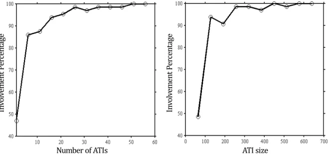
continuous TI and the histograms of 50 realizations, conditional to 100 HD, obtained with and without ATIs. . . 53 Figure 3.16 ATI involvement in simulation as a function of the number of (size 64
× 64) ATIs (left), or the size of a single ATI (right) for the continuous TI of Fig. 3.13. Values on X axis in right figure are the dimensions of ATI along both X and Y directions (e.g., 100× 100 or 200 × 200). The simulations performed with T =6 and OL=2. . . . 55 Figure 3.17 Simulation using a small TI with T =8 and OL=3 . . . . 56 Figure 3.18 Simulation results for the channel image with T = 15, and OL = 5.
Red circles HD belong to channels and the blue ones to non-channel facies . . . 57
Figure 3.19 Variograms along X direction (A) and Y direction (B) for the 25 rea-lizations (light gray) and the OTI (black), channel TI displayed in Fig. 3.9-D. . . 58 Figure 3.20 E-type maps of 25 realizations produced with and without ATIs, T =10,
OL=3. OTI obtained from Fig. 3.18. . . . 59 Figure 3.21 Simulation results using three-facies OTI with ATI (middle row) and
without ATI (bottom row), T =17, and OL=6. . . . 60 Figure 3.22 Simulation results using 3D ball TI with T =15, and OL=5. . . . 62 Figure 3.23 Simulation results using continuous 3D TI with T =15, and OL=5. . . 63 Figure 3.24 CPU time. Top row, left, dashed line: 2D simulations, ATI size varies
and simulation grid size is fixed at 64× 64; solid line: simulation grid varies and TI size is fixed at 64 × 64. Top row, right, dashed line: 3D simulations, ATI size varies and simulation grid size is fixed at 50× 50 × 50; solid line: simulation grid varies and TI size is fixed at 50× 50 × 50. Bottom row: the number of ATIs varies, each ATI and simulated field of size 100× 100 × 100. For 2D simulations T = 10 and OL = 4; for 3D simulations, T = 15 and OL = 5. . . . 64 Figure 4.1 Right: Binary HD and three soft data sets; Left: Probability field
obtained by multinomial logistic regression. . . 73 Figure 4.2 Left: HD and soft data map; Right: probability fields for three categories. 74 Figure 4.3 The TI used to generate the reference model on top row. Left column:
original soft data used as input in logistic regression; middle column: probability of facies 1 (black); right column: e-type map of facies 1 of 50 realizations based on the probability fields. Note the HD are not displayed on the figure, but they are used in all the simulations. Input parameters: weak case: α=0.12, medium case: α=0.31, strong case: α=0.68. Average patch size and overlap width are 15 and 5 respectively. Np = 10. . . 77 Figure 4.4 Simulation results using the ball TI with different probability fields
(colorscale: white-1, black-0). Average patch size and overlap width are 15 and 5 respectively. α = 0.4, NP = 10. . . 78 Figure 4.5 TI and two sample simulations (first row) conditioned to probability
fields (second row); e-type maps of 25 realizations (third row) and variograms (bottom row). Average patch size and overlap width of 15 and 5 respectively; α = 0.45, Np = 50. . . 80
Figure 4.6 One conditional realization (right column) using the probability fields in the first two columns for the multifacies TI shown on top, (colorscale: white-1, black-0). The bottom row displays the e-type map per facies for 100 realizations using probability fields shown above in the fourth row. Average patch size and overlap width are 15 and 5 respectively. α = 0.4, NP = 10. . . 81 Figure 4.7 TI (top row), two soft data and probability fields (second row),
refe-rence model, one realization and e-type map based on 10 realizations (third row), variograms (fourth row) and L2-functions (fifth row) of the reference and the 10 realizations. Average patch size and overlap width of 35 and 12 respectively, α = 0.52, Np = 100. . . 83 Figure 4.8 3D ball TI and the probability field were used to perform 25
conditio-nal simulations. One sample simulation and the e-type cubes are also displayed. Size of the TI and simulation grid are both 50*50*50. Ave-rage patch size and overlap width are 16 and 5 respectively. α = 0.60, Np = 100. . . 84 Figure 4.9 A: 3D channel TI, B: probability volume, C: sample simulation and D:
e-type map of 25 realizations. Average patch size and overlap width are 30 and 10 respectively. α = 0.4, NP = 100. . . 85 Figure 4.10 Top row: TI, the probability field and one sample ATI (out of 10) used
for the simulation; second to fifth rows: one sample realization (left), e-type map (middle), correlation plots (right) for α = 0.0, 0.1, 0.4 and 0.7. Each e-type map is computed from 25 realizations (colorscale: white-1, black-0). ATIs are unconditional patch-based simulations of TI using quilting (El Ouassini et al, 2008; Faucher et al, 2013). Average patch size and overlap width are 20 and 7 respectively. Np = 25. . . . 86 Figure 4.11 Correlation between e-type and probability field as a function of the α
parameter. E-type map computed from 25 realizations for the TI and probability map shown in Fig. 4.10. . . 87 Figure 4.12 Sensitivity of the simulations to the weights given to HD (β) and soft
data (α); C represents the % of HD reproduced (colorscale: white-1, black-0). C values are calculated over 10 realizations for a bet-ter estimate of HD reproduction. Size of the TI and simulation grid are 200*200 and 250*250 respectively. Average patch size and overlap width are 24 and 8 respectively. Np = 25. . . 89
Figure 4.13 TI, one realization and e-type maps based on unconditional (middle row) and conditional (bottom row) realizations; HD as red dots; ave-rage patch size and overlap width 25 and 9 respectively. α = 0.4, Np = 25. . . 90 Figure 4.14 Mallik area, Mackenzie Delta, Northwest Territories, Canada;
bore-holes, and area covered by tomography and seismic investigations. Fi-gure borrowed from Dubreuil-Boisclair et al (2012). . . 92 Figure 4.15 Correlation in 2L and 5L borehole logs of methane hydrate grade and
seismic velocity. . . 93 Figure 4.16 Top row: Original TI obtained by thresholding Vp at 75th and 85th
percentiles; bottom row: two large ATIs generated by unconditional simulation using the original small TI. A total number of 25 ATIs were used for the simulations. . . 94 Figure 4.17 Top left: original soft data (inverted Vp), top right and bottom row:
probability field per category (colorscale: white-1, black-0); on each category probability field the points in boreholes belonging to the same category are overlaid, α=pseudo-R2 = 0.14. . . . 95 Figure 4.18 Three conditional simulations randomly selected from 100 realizations.
Average patch size and overlap width are 8 and 3 respectively. α = 0.14, Np = 25. . . 96 Figure 4.19 Left: Probability fields for the three categories; Right: e-type maps per
category based on 100 realizations. . . 97 Figure 5.1 Top left: TI generated with an object-based simulation method
(To-tal, 2016); middle left: one realization with 20 ATIs; bottom left: one realization using only the TI, 250 HD indicated. Top right: HD re-production rate for 50 different realizations with and without ATIs. Bottom right: L2 function for the 50 realizations obtained with and
without ATIs. . . 104 Figure 5.2 Dunes TI from Allard et al (2011) (top left); lithotype template
(bot-tom left); two MPS unconditional realizations (second column from left) and corresponding Gaussian fields (two rightmost columns) . . . 106 Figure 5.3 GDM applied on the dunes TI. The two input realizations are the ones
on second row far left column and lower right sub-figures. These are merged using different weights shown on top of each sub-figure. . . . 108 Figure 5.4 Two realizations (left), original and cleaned merged realizations. The
Figure 5.5 Proportion map test case. First row: from left to right, two sample MPS simulations, reference map and the final GDM model. Second row: grey facies proportions. Last row: white facies proportions. GDM applied with parameters m=200, n = 2, k=4, g=110, mk=20, mb=10. 111 Figure 5.6 Proportion map test case. First row: Reference and target proportion.
Second to last rows: best merged calibrated realisation obtained at different generations. GDM applied with parameters m=500, n = 2, k=4, g=50, mk=20, mb=10. . . 113 Figure 5.7 Proportion map test case. First row: Target proportion and e-type
over 50 realizations. Second row: four different calibrated GDM rea-lizations. GDM applied with parameters m=500, n = 2, k=4, g=50, mk=20, mb=10. . . 114 Figure 5.8 Travel time test case. P: producer well. Travel times between injector
and producers are given for reference field, two sample MPS realizations and GDM output. Misfit shown on the rightmost sub-figure. GDM applied with parameters: m=50, n = 2, k=4, g=50, mk=20, mb=10. . 115 Figure 5.9 Seismic section calibration example. Elastic properties and wavelet:
bottom left sub-figure, misfit of input MPS and GDM-calibrated: bot-tom right. GDM applied with parameters: m=500, n = 2, k=3, g=500, mk=20, mb=10. . . 116 Figure 5.10 TI selected from Maules Creek Australia (left) and reference shortest
paths between injector-receivers (right). . . 118 Figure 5.11 Shortest path travel time 3D example. Top: sample initial MPS
rea-lization, middle: reference, bottom: one GDM-calibrated realization. The misfit of input realizations are displayed in the bottom figure as compared to the GDM final model misfit. GDM applied with parame-ters: m=50, n = 3, k=4, g=40, mk=20, mb=10. . . 119 Figure 5.12 Two-phase 2D water cut example. Water saturation (top left),
re-ference (top right), one initial MPS realization (bottom left), GDM calibrated realization (bottom right). GDM applied with parameters: m=50, n = 2, k=4, g=10, mk=10, mb=5. . . 120 Figure 5.13 Water cut curves at wells P1 to P3 for two initial MPS realizations
(left) and GDM-calibrated realization (lower right). Misfit values of 50 MPS realizations and GDM-calibrated realization (upper right). . . . 121
Figure 5.14 Two-phase 3D water cut example. Water saturation (top left), re-ference (top right), one initial MPS realization (bottom left), GDM calibrated realization (bottom right). GDM applied with parameters: m=50, n = 2, k=4, g=13, mk=10, mb=5. . . 123 Figure 5.15 Water cut curve at the well P1 for the best GDM model after Ng
generations. . . 124 Figure 6.1 The TI was used to create the reference model from which the hard
data on right are extracted. . . 128 Figure 6.2 Three layers of soft data. The areas highlighted with colored rectangles
refer to the correlation between soft data values and facies coding. Red boxes highlight the areas where F1 and higher values of soft data correlate positively, and the opposite for light blue rectangles. . . 128 Figure 6.3 Three soft data layers on top are merged in different ways generating
probability fields of F 2. S1 to S3 refer to soft layers 1 to 3, and P (S1 + S2) means the probability calculated with soft layers 1 and 2. 130 Figure 6.4 The influence of different combination of soft data in classification results.131 Figure 6.5 Reservoir grid extracted from the reference model used for flow
simu-lations. The variations of TOF values on base 10 logarithmic scale. . 132 Figure 6.6 Water cut curves at production wells. One time unit on the X axis
counts for 121 days totalling a 10 years time period of flow simulation. 133 Figure 6.7 The original TI and three randomly selected ATIs. . . 134 Figure 6.8 The sample realizations conditioned to hard data only. The e-type map
for 100 realizations. . . 135 Figure 6.9 Box-plot of conditioning rates of 100 realizations with and without ATIs.136 Figure 6.10 Sample simulation conditioned to soft data only. The e-type map for
100 realizations. The Pearson correlation coefficient between e-type map and input proportion map is 0.85. . . 137 Figure 6.11 The models conditioned to hard and soft data at the same time. The
Pearson correlation coefficient between e-type map and input propor-tion map is 0.72. . . 138 Figure 6.12 Time Of Flight (TOF) and drainage patterns in reference model (A),
unconditional simulation (B), hard conditioned model (C), soft condi-tioned model (D) and hard and soft condicondi-tioned model (E). . . 140 Figure 6.13 Shown on top are TI and the lithotype template (upper right), with
three sample realizations on bottom over the reservoir grid with cor-responding Gaussian variables. Realizations are the same as Fig. 6.11. 142
Figure 6.14 The dynamic response of set of realizations conditioned to hard data only (first row), conditioned to soft data only (second row), both and hard and soft data (third row) and GDM output (fourth row). GDM was used with parameter setting of m=400, n = 1, k=3, g=100, mk=20, mb=10. . . 144 Figure 6.15 The water rate curves at the producers in three GDM outputs as
com-pared to the water rates reference model. GDM was used with para-meter setting of m=400, n = 1, k=3, g=100, mk=20, mb=10. . . 145 Figure 6.16 TOF and drainage patterns of the reference model (top row) and three
LIST OF INITIALS AND ABBREVIATIONS
MPS Multiple-Point Statistics TI Training Image
ATI Alternative Training Image OTI Original Training Image
HD Hard Data
T Template size OL Overlap size
GDM Gradual Deformation Method EnKF Ensemble Kalman Filter
τ Tau factor
d(P, S) Distance between P and S P Data event from TI
S Data event from simulation grid w Weighting matrix in distance function O Objective function response
r Deformation factor
α Soft data weight in distance function ∗ Convolution function
⊙ Hadamard product
E Cumulative error function χ2 Chi-squared test
P (k|x) Probability of category k in the presence of soft data x pT I Proportion in the patch from TI
pSI Proportion in the patch from probability map R2 McFadden’s pseudo regression coefficient
Lc Likelihood of the full model fitted with soft data
L0 Likelihood for the null model having only the constant term
β Weight given to hard data
Np Number of patterns in the pool of candidates Z Latent Gaussian variable
n Number of latent Gaussian variables from each facies model m Number of MPS realizations in a given generation
mk Number of merged realizations produced for each generation mb Number of best realizations
g Number of generations dm Merged model data do Observed data mD Milli Darcy cP Centi Poisse sW Water saturation
CHAPTER 1
INTRODUCTION
1.1 Facies Modeling
Facies modeling refers to the population of discrete property values on the geocellular grids in hydrocarbon reservoirs, mineral deposits or groundwater aquifers. The primary variables of interest such as permeability, porosity or ore grade often show different distributions in different facies. Given that petrophysical properties highly correlate with facies type, facies data are available on well logs or boreholes, and facies data are spatially correlated, it is recommended to start with a facies modeling step before continuous property modeling such as porosity and permeability (Pyrcz and Deutsch, 2014). Facies modeling techniques can be labelled as either deterministic or stochastic. Deterministic approaches like Indicator Kriging (Journel, 1983) gives one fixed value per pixel in all estimation runs. Such models are preferred when enough input facies data are available such that there is no need for generating multiple realizations of the underlying ground truth geology. On the other hand, stochastic methods like sequential indicator simulation (SISIM, Deutsch and Journel 1998) generate in different simulation runs different realizations of the random function governing reservoir or mineral deposit geology.
Stochastic methods are interesting choices since the set of multiple realizations can be used for uncertainty assessment and they do not suffer from the smoothing effect of the Kriging-based estimation techniques. Examples of stochastic methods include object-Kriging-based simula-tions (Damsleth et al, 1992; Shmaryan and Deutsch, 1999; Deutsch and Tran, 2002), se-quential indicator simulation (Deutsch and Journel, 1998), multiple-point statistics (MPS) (Guardiano and Srivastava, 1993; Strebelle, 2002), truncated Gaussian simulation (Le Loch and Galli, 1997; Galli et al, 1994) and process-based algorithms (Koltermann and Gorelick, 1992; Pyrcz et al, 2009). The spatial correlations are quantified within object distribution pa-rameters, variograms and training images (TI) in object-based, truncated Gaussian and MPS methods respectively. The set of multiple realizations should give an idea of what the spatial facies distribution looks like. For example such realizations of the subsurface can be used in flow modeling in reservoir or hydrogeology to determine the range of expected variations of fluid flow behaviour of realizations (Koltermann and Gorelick, 1996).
1.2 Why Using MPS ?
The central idea in MPS is to infer the multiple point cumulative distribution functions (CDFs) from a TI rather than from a variogram.The TI can be seen as a realization of an undescribed random function in the head of the geologist. In the classic Kriging-based geostatistics, the estimation is based on a variogram that measures the spatial correlation between data samples. Such variogram is empirically obtained from the observed data. Ho-wever, variogram inference, particularly along the horizontal direction, most of the time is not possible due to the wide horizontal spacing between wells or boreholes. In such cases it is inferred from other sources such as seismic data inverted for acoustic impedance elastic property (Chambers and Yarus, 2002; Francis, 2005; Deutsch and Journel, 1998). Variograms can also be borrowed from TIs depicting the expected geological structures from analogues, direct geological maps, outcrops, satellite imagery data, etc. Even if variogram is available, the output realizations often lack geological realism (see Fig. 1.1). As stated in Mariethoz and Caers (2014) "We now need to recognize that in practice, what is often ultimately desired is not a multivariate distribution and its parameters estimates, but the realizations generated." referring to the fact that the realism of the output models is more important than the beauty of the mathematical model used. The limitations of variogram in capturing curvilinear conti-nuities as in meandering channels, and conditioning problems of object-based algorithms led to the advent of MPS method with Guardiano and Srivastava (1993) and later on with a more practical version of it with Strebelle (2002).
As mentioned above, at the core of MPS is a TI deemed as an example or a realization of geology ones expect to see in the subsurface and is used to convey conceptual or observed geological heterogeneities from field to facies simulation. In this regard, a TI can come from geological sketches, satellite imagery data, extracted mine levels, or object-based simulations. Using TI rather than a variogram results in considerable improvement of geological realism of facies simulators outputs. An example is provided in Fig. 1.1 depicting meandering channels host to hydrocarbon fluids. The reference channel model is displayed on top left of the figure. The reservoir is hit with three producers (P 1 to P 3) and one injector well (I1). One conditional realization was produced using an MPS algorithm shown in the middle row, and one with a variogram-based simulation technique namely SISIM.
The channel was considered as permeable and more porous than the background shale (per-meability values shown in Fig. 1.1). As can be seen in the reference model the channel between I1 and P 1 is the shortest path of fluid flow as depicted with the time of travel on the right figure. The model produced with MPS connects very well I1 and P 1 in that the shortest path between I1 and P 1 is through the connecting channel in between. However, the SISIM flow
response is significantly different than the reference as in this model there is no preferential path between I1 and P 1 and fluid has been dispersed to P 2 and P 3 producers as well.
Figure 1.1 The significant difference between the flow response of channels simulated with SISIM and MPS. The facies models on left column are colored with permeability values. The right column shows the travel time (in logarithmic scale) between source and sink.
The idea of using a TI rather than a variogram is elegant and in most cases, MPS outperforms Kriging-based algorithms, however its application is still limited due to some main problems. First is the availability of a TI. TIs can come from variety of sources however one that is representative for the sub-surface heterogeneity can be cumbersome to acquire. Second is the compatibility of conditioning data with the TI. If the hard data observed on the well logs
do not match with the patterns and structures of TI, conditional facies modeling can be an extremely tedious task. In many cases an object-based simulation (Damsleth et al, 1992; Jones and Larue, 1997; Deutsch and Tran, 2002) can be an excellent choice to produce a TI. The application of object-based simulation directly for facies modeling can be limited due to the conditioning problems to dense hard data, or even soft data such as proportion or orientation maps. Facies modeling can be performed using the process models (Xie et al, 2001; Pyrcz and Deutsch, 2005; Pyrcz and Strebelle, 2006; Reza et al, 2006). Such methods are based on the physical and chemical processes that govern the geological settings of the phenomena under study. Process-based algorithms can generate facies models that are very realistic in terms of their structural contents but the computational efficiency and conditioning can be problematic (Michael et al, 2010). However, process-based models can perfectly serve as TI in MPS given that such models are stationary, are not repetitive, and structural complexity of process-based models are not challenges for this use.
1.3 MPS Workflow
Having provided a representative TI, MPS follows a sequential simulation process in which data events are extracted from the simulation grid from within the neighbourhood of the simulation point. Data events can contain hard conditioning data, soft conditioning data and/or previously simulated cells. In the next step TI or its corresponding pattern database (namely search tree) is searched using the extracted data event for the matching facies coding. Consider the TI on Fig. 1.2 left with 10×10 pixels of sand channel (black) and background shale (orange). Also consider the 2D simulation grid on right here with same size as TI. There are few conditioning data assigned on the simulation grid in advance. A search window of a specific size is defined ; here it is a circle of radius two pixels. The path through which nodes are visited for simulation can be random or unilateral (here random, for unilateral see Fig. 1.5). At each node under simulation, informed nodes are extracted from search neighbourhood of simulation point. This data event is used to search the TI for matching patterns. In some MPS algorithms such as SNESIM (Strebelle, 2002), IMPALA (Straubhaar et al, 2011) and SIMPAT (Arpat and Caers, 2007), a pattern database of all patterns present in the TI is constructed in advance so that the TI does not have to be scanned anew for each node. Or the TI can be scanned all at once using distance functions calculated with cross correlation functions as in CCSIM algorithm (Tahmasebi et al, 2012) or convolutions as in Rezaee et al (2015). The other idea is to search in the TI on random locations and match the data event from simulation with the local patterns in TI, and take the first matching pattern as in Direct Sampling method (Mariethoz et al, 2010). In either case, the simulated facies the
simulated facies cpdf (conditional probability distribution function) is read from the TI and a simulated value is drawn and pasted to the simulation point. Simulation is moved on to the next uninformed node until all nodes are visited. In some algorithms an iterative process is proposed so that the simulation points that are simulated with smaller than a threshold number of informed nodes in their neighbourhood are re-simulated (SNESIM). In patch-based algorithms the whole field is re-simulated using smaller and smaller patches (Efros and Freeman, 2001).
Figure 1.2 The basic idea behind MPS simulation.
Patch-based algorithms simulate better the texture of facies as observed in the TI because of simulating patches of facies values taken from TI and transferred to the simulation window. It also preserves the short-range variations of the variable in TI since they are exactly copy-pasted from the TI to the simulation field. On the other hand, in pixel-based algorithms, short-range fluctuations can be observed in the simulated field which are different from those present in the TI and are due to simulating one point at a time.
1.4 Patch-based MPS
As mentioned above MPS algorithms can be classified into pixel-based and patch-based simulations (see Fig. 1.3). The pixel-based approach simulates one node at a time while patch-based simulates a bunch of nodes similar to object-based algorithms. Patch-based al-gorithms follow generally a unilateral simulation path, while pixel-based can be done either with a unilateral or random path. Patch-based simulations with random path often present
artefacts and discontinuities. The patch-based unilateral algorithms bear a greater potential at reproducing better the texture of TI. Figure 1.4 shows an example where the texture of patch-based algorithm resembles more the texture of TI. With a fixed template size (T ), the overlap size OL is continuously increased, i.e., smaller number of pixels simulated at once, i.e., (T − OL)2. The quality of simulation decreases as the the number of points simulated
simultaneously decreases. Note that T = 5 and OL = 2 in Fig. 1.3-right.
Figure 1.3 Patch-based vs. pixel-based MPS simulation.
Figure 1.5 displays few iterations of a unilateral patch-based MPS simulation based on dis-tance functions as in Rezaee et al (2015). At the top a TI of channels and an empty simulation grid (unconditional case) are displayed. In step (1) since there are no informed nodes in the simulation grid, distance function gives the same chance for all patterns in TI to be picked, therefore one random pattern from TI is selected and pasted on the top-left corner of the simulation grid. In step (2) however, parts of the simulated patch in step (1) are used as over-lap to calculate its distance with the TI. The overover-lap region is highlighted with red rectangles in iteration (2) and (3) as well. The most similar or one pattern in the pool of candidate patterns in the TI is selected based on the distance map (highlighted with red plus sign) and is pasted to the simulation grid. This process continues until all nodes of simulation grid are simulated.
1.5 Potential problems with patch-based MPS
One potential pitfall of patch-based MPS simulations is the verbatim copying effect observed in set of all similar simulations that lack between-realization variability. This effect can be observed particularly with small TIs. One possible solution lies in using larger multiple set of
Figure 1.4 Pixel-based vs. patch-based approaches in generating texture. Simulation using T=22 and OL=21 is a pixel-based simulation since the size of patch is reduced to only one pixel. Simulations are performed using distance-based approach based on quilting and a unilateral simulation path.
TIs. The approach presented in Chapter 3 on using multiple TIs is a step forward obviating this problem of patch-based MPS.
Better reproduction of texture in patch-based MPS algorithm is associated with inherent conditioning problems. Especially in presence of dense hard data. As it will be demonstrated in the next chapter, the probability of finding matching pattern in a given TI for a data event from simulation grid drops rapidly to zero as the number of conditioning data within the patch increases. This is similar to object-based simulation where in the conditioning process to dense hard data (particularly along vertical direction) inconsistencies occur between previously simulated objects and new ones. One solution lies in enriching the TI and simply generating more patterns such that one would match the data event from simulation grid. This problem is addressed in more details with a review of the literature in Chapter 3.
Soft data conditioning is not specific to patch-based simulation but to all MPS methods and other facies modeling tools as well. The main issue here is that the physical relationship between soft data and facies types is often unknown, yet during the simulation using a MPS technique, they are taken as direct proportion maps in most cases. One has to get the
Figure 1.5 Patch-based MPS simulation using distance functions. It is not necessarily the pattern in TI corresponding to minimum distance that is selected, but instead a pool of pattern is first formed from the lowest distance values, and one pattern is picked at random and pasted to the simulation grid. The red plus sign shows the upper left corner location of the selected pattern and three white dots on the distance map indicate other three corners.
proportion maps from soft data sets in the first place. Soft data are often given in the form of multiple geophysical maps/cubes. With hard data labelled with facies types from well logs for example, one can perform a supervised classification between hard data and their overlaying soft data, and extend the regressed model to the rest of the simulation grid where only soft data are present. Among the techniques for supervised classification we propose using Logistic Regression model. The reason lies in the pseudo-R2 of McFadden (McFadden, 1973) that can
be used as a weighting factor given to soft data component of the similarity measure in MPS simulation, and also the simple implementation of logistic regression classification. Also, when applying logistic regression, there is fewer number of parameters that requires tuning. Chapter 4 addresses this problem with first a literature review of the available methods in this regard.
The third problem is the conditioning of MPS (or other facies simulators) facies models to dynamic data. Dynamic data are global and depend on larger areas than soft data around the conditioning data, namely wells. The direct history matching of facies is an arduous task in that the facies are defined with categorical type variables, their perturbations can deform severely the covariance model of the field. The technique we used is based on the Gradual Deformation Method, modified into an evolutionary algorithm. We propose deforming the latent Gaussian variables of the facies realizations using a Gibbs Sampling (Geman and Geman, 1984) technique as in PluriGaussian simulation (Le Loch and Galli, 1997). The perturbations are instead performed on the Gaussian fields, and their outcome is truncated using a lithotype flag defined from the TI. The new perturbed model is forward modelled whose fitness is checked with target variable. The best fitted realizations survive to the next generation of realizations. Next chapter provides more details on GDM technique and other related approaches on this problem.
CHAPTER 2
PROBLEM STATEMENT AND LITERATURE REVIEW
2.1 Elements of the Problem
Facies simulation is an important step in reservoir, mineral deposit or groundwater aquifer modeling in that further simulation of continuous properties can be improved considerably knowing what facies we are in. Among the facies modeling tools, MPS has become a popular choice since it conveys the geological information from geologist directly to the simulation grid; however as indicated in the previous chapter, it faces conditioning problems when it comes to dense hard conditioning data, multiple soft data layers, or global dynamic data. In this chapter these problems are extended to more details.
2.1.1 Hard Data Conditioning
Hard data refer to the direct observation on the wells or drill holes of facies or measurements of continuous properties such as resistivity, density, ore grade, etc. Their resolution on the vertical direction can be as fine as few centimetres in reservoir, and fractions of a meter in mining; and on the horizontal direction up to hundreds of meters to few kilometres in reservoir or tens of meters in mining. The facies model must be conditioned to the hard data. After the simulation grid is defined, before the simulation starts, hard data are relocated on the regular simulation grid. During the simulation, data events are extracted from the simulation grid and their similarity is measured with the TI. Data events from simulation grid come with previously simulated data and/or hard data. The values from the TI often do not match the entire set of existing cells in the simulation grid. Pixel-based and patch-based approaches handle the problem differently. In the former, both hard data and the overlap nodes are fixed during the simulation, i.e., one simulated value will not be overwritten with any new value until the end of simulation. Previously simulated parts are taken exactly the same as conditioning data. In patch-based simulations however, the data on overlap region can be changed during the simulation, but the hard conditioning data are fixed during the simulation. It is highly possible that the simulated value over the hard data or overlap does not perfectly match the pre-existing values. The problem is more severe for patch-based MPS similar to object simulations. The problem occurs when TI does not have enough repetitions of patterns in enough varying configurations, or when the data event is too large for the TI. A number of techniques have been proposed to the problem of hard data conditioning in
MPS. In most MPS algorithms, hard data are fixed on simulation grid before simulation starts and not changed thereafter. During the course of simulation if TI does not have any matching pattern for data event, the farthest nodes are dropped one at a time and the distance/conditional probabilities are re-calculated (Strebelle, 2002). If the reduced data event still does not have any matching pattern in TI, another node is dropped. This process continues until at least one matching pattern is found. In methods like DS (Mariethoz et al, 2010) which is based on distances rather than probabilities, output distance value is normalized between a minimum and maximum value [0-1], a threshold (e.g., 0.05) on the distance function then determines if the pattern in TI will be pasted to simulation grid or not. In case such matching pattern is not found, the best matching pattern so far stored in the pattern database is selected and pasted to the simulation grid even if the distance is well above the threshold.
In patch-based algorithms, the problem becomes harder as it is now to condition a patch of nodes simultaneously to conditioning data. In the method CCSIM (Tahmasebi et al, 2012) for example, when the matching pattern is not found, the square-shaped patch is divided into four small complementary patches, each are tested against TI for matching patterns using cross correlation functions. If for any of the smaller parts the match is not yet found, it is divided into another four smaller pieces again and this continues until the matching pattern is found in the TI which is guaranteed to find for only one pixel remained in the patch in the end of the process (see Fig. 2.2).
Window enlargement technique was proposed with Parra and Ortiz (2011) in pixel-based MPS based on a texture synthesis method borrowed from the computer graphics (Wei, 2002). During the simulation, a larger area than the usual search neighbourhood is scanned to find the nearby (but not in the simulation window) hard data, such that the algorithm foresees the forthcoming hard data, and pastes beforehand the patterns from TI that are readily compatible with the nearby hard data. The idea was adopted with Faucher et al (2013) and Rezaee et al (2015) to enhance the conditioning capabilities of patch-based simulations. However, if the TI is not rich, the chance of finding a matching pattern for an enlarged window is even slimmer.
As mentioned above, in case of non-matching data events from simulation grid and simulated values from TI, the most frequent idea is to reduce the size by dropping the farthest nodes iteratively until matches are found. The plot on Fig. 2.2, shows for three different TIs the portion of the original data event that has to be discarded until a matching pattern is found in the TI. More than 50% of the data event are discarded when the data event has only 50 pixels; more than 80% are discarded of the data when the size is 100 pixels or more. In other words 80% of the data from simulation grid are not used in the pattern matching step. One
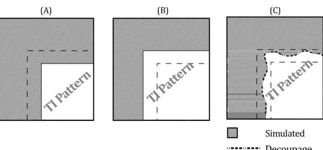
Figure 2.1 The recursive template splitting idea as used in CCSIM (Tahmasebi et al, 2012). The original template with overlap regions in gray and the parts to be simulated in green are highlighted in the simulation grid on left. Right column shows the process through which the original template is split recursively until the matching pattern is found in TI.
hundred pixels counts for a square search window of 10×10 while in practice much larger templates are required for most of the simulations. DS method scans only a portion of TI for faster computations, e.g., 50 % of the TI. The chance of finding a match within the portion of TI gets smaller than the case when the whole TI is scanned.
In all solutions presented, there is a data reduction mechanism, either in the form of template splitting, of farthest node drop out or in the form of similarity measure compromise as in the DS method. However, the degree of severity of the problem is high as shown in Fig. 2.2 where in the most optimistic case, only 50 % of the original data event’s pixels are used to calculate the conditional probability from TI using distances or counting the number of replicates. To this problem we rather propose to enrich the TI and keep data event untouched. One solution is to take as input not only one TI but a series of TIs. Such Alternative TIs (ATIs) can be unconditional simulations using the original TI (OTI) of any size and number as long as CPU time allows. To this end the test in Fig. 2.2 was repeated once only with OTI and next with OTI+10ATIs. ATIs were unconditional simulations over the same grid size as OTI using a patch-based algorithm based on quilting (Efros and Freeman, 2001). The results are displayed in Fig. 2.3 where using 10 ATIs increases the chance of finding a matching pattern and reduces the portion of data that has to be dropped out to find a matching pattern. ATIs are more influential for the multi-facies channel TI shown in Fig. 2.3-C directly due to the increased number of facies.
In this test (Fig. 2.3) there was no control over the ATIs in terms of their pattern content and diversity, compatibility with hard data, and similarity to OTI. Such ATIs come with little effort in terms of CPU time or input parameters tuning since they are unconditional simulations using patch-based MPS where the most important parameter is to select the proper patch size. We propose to generate ATIs in large numbers but to retain only the fittest ones for the main conditional simulation.
Conditioning of patch-based MPS algorithms to dense hard data is a problem, as the TI in most of the cases is not responsive to all data events coming from simulation grid. The first objective is this dissertation seeks the solution in enriching the TI’s pattern database with ATIs. The efficient way of generating and using ATIs and sample results is studied and presented in more details in Chapter 3.
2.1.2 Soft Data Conditioning
Soft data are linked in often an indirect way to the facies distribution. They are mainly obtained by geophysical prospecting and further data processing and modeling (e.g. seismic inversion). Soft data can sample different areas from the hard data, or reflect different features of the subsurface geology. They inform about the local abundance of the different
Figure 2.2 Top: three selected TIs, bottom-left: probability of finding a perfect matching pattern from the TI vs. data event size, bottom-right: portion of the original data event that has to be droped out until we find a matching pattern in the TI.
Figure 2.3 Same test as in Fig. 2.2 repeated with and without ATIs. The probability of finding a matching pattern on left columns and the portion of original data event dropped out to find a matching pattern as a function of data event size for channel TI (A), dunes TI (B) and multi-facies channel TI (C), see Fig. 2.2.
facies (at the scale of resolution of the geophysical data). Hence, they can be used to allow proportion of facies to vary in space. One method to link facies probabilities obtained from TI and MPS to facies probabilities obtained from soft data is thru the method of aggregation of probabilities. Allard et al (2012) give an excellent review of available methods. All these methods seek to simplify the computation of conditional probabilities.
Consider A as facies observation at node u under simulation, B data event around u, and C soft data within the search window. In a case of conditioning to hard data only, one needs to calculate the conditional probability of A which is solved in the form of Bayesian inference problem with P (A|B) = P (A, B)
P (A) as described in Strebelle (2002). With soft data however, we have P (A|B, C) = P (A, B, C)
P (B, C) that becomes more complicated to calculate the joint probability between B and C. One way to account for soft data in MPS simulation has been the use of Tau model (Journel, 2002) in a probability aggregation method (Allard et al, 2012). In the Tau model (Eq. 3.1):
x b = (c a )τ (2.1) with a = 1− P (A) P (A) , b = 1− P (A|B) P (A|B) (2.2) c = 1− P (A|C) P (A|C) , x = 1− P (A|B, C) P (A|B, C) (2.3)
where P (A) would be the marginal probability of facies indicator in TI. The conditional probability P (A|B, C) has become a function of P (A) and two probabilities of A separately conditioned to B and C. P (A|B) is the conditional probability of data event in search neighbourhood in simulation grid, and P (A|C) is the soft data conditional probability. The factor Tau (τ ) is an indicator of the redundancy between B and C (Krishnan et al, 2005). In practice defining the degree of redundancy between B and C is very difficult and moreover it has to be done on every single simulation node. For these reasons τ = 1 is used in most practices. Figure 2.4 shows an example of the conditional simulation using the Tau model. In this figure we have as inputs a channel TI, one rotation map and the proportion map of channel facies as soft data. The simulations are repeated with τ = 1, τ = 50 and τ = −5. As can be seen higher τ values forces more the soft proportion condition as in the case of τ = 50 the e-type map does not show much uncertainty. Negative τ values reverses the effect of soft data in that the e-type map shows inverse relationship to the soft proportion map.
Figure 2.4 The TI, rotation map and the proportion maps were used to perform conditional simulations. Sample simulations are presented with different Tau values. With permission from Liu (2006).
Non-stationarity has been handled in the form of auxiliary variables as in Chugunova and Hu (2008) and Mariethoz et al (2010). Chugunova and Hu (2008) implement conditioning to auxiliary data in SNESIM algorithm (Strebelle, 2002) by constructing a search tree of
patterns not only of primary TI but also auxiliary variable TI. The pattern configurations to build the database or search tree for soft data are the same as for the primary TI (facies TI) search tree. In a sequential simulation, at each node data events are extracted from the neighbourhood of the simulation point; candidate patterns are identified from the principal variable TI’s search tree, and among the set of candidates are selected only those that satisfy the auxiliary data condition too that comes from the auxiliary data TI on the simulation point. In this context auxiliary data could be proportion of facies within the search window, orientation of the objects, other geometrical features of facies. Figure 2.5 shows an example of the simulation conditioned to the proportion maps as auxiliary data. The reproduction of soft proportion data in the e-type map is fairly good. The patterns in the simulation (Fig. 2.5-C) is also similar to TI. Figure 2.6 shows an example of a TI of fracture network, the orientation map showing azimuths of 0 to 90 degree and the sample simulation.
Figure 2.5 A: TI, B: auxiliary variable, C: sample simulation and D: e-type map of 50 real-izations. With permission from Chugunova and Hu (2008).