A REGULARIZED INTERIOR-POINT METHOD FOR CONSTRAINED LINEAR LEAST SQUARES
MOHSEN DEHGHANI
D´EPARTEMENT DE MATH´EMATIQUES ET DE G ´ENIE INDUSTRIEL ´
ECOLE POLYTECHNIQUE DE MONTR ´EAL
M ´EMOIRE PR ´ESENT´E EN VUE DE L’OBTENTION DU DIPL ˆOME DE MAˆITRISE `ES SCIENCES APPLIQU ´EES
(MATH´EMATIQUES APPLIQU ´EES) AVRIL 2013
c
´
ECOLE POLYTECHNIQUE DE MONTR´EAL
Ce m´emoire intitul´e :
A REGULARIZED INTERIOR-POINT METHOD FOR CONSTRAINED LINEAR LEAST SQUARES
pr´esent´e par : DEHGHANI Mohsen
en vue de l’obtention du diplˆome de : Maˆıtrise `es sciences appliqu´ees a ´et´e dˆument accept´e par le jury constitu´e de :
M. LE DIGABEL S´ebastien, Ph.D., pr´esident
M. ORBAN Dominique, Doct. Sc., membre et directeur de recherche M. VIEIRA Manuel Valdemar Cabral, Doctorat, membre
To Who has taught by the pen. He has taught man that which he knew not. . . (From the Holy Quran, Surah : 96, AL-Alaq, Verse : 4-5)
ACKNOWLEDGEMENT
This research project would not have been possible without the support of many people. The author wishes to express his gratitude to his supervisor, Prof. Dr. Dominique Orban who was abundantly helpful and offered invaluable assistance, support and guidance. Deepest gratitude is also due to the members of the Jury committee, Prof. Dr. Le Digabel S´ebastien and Prof. Vieira Manuel, and his brother Ahad Dehghani without whose knowledge and assistance this study would not have been successful. Special thanks also to all my friends, especially my GERAD friends for sharing invaluable assistance.
The author wishes to express his love and gratitude to his beloved family members for their understanding throughout the duration of his studies.
R´ESUM´E
Nous proposons une m´ethode de points int´erieurs non r´ealisable pour le probl`eme aux moindres carr´es lin´eaire avec contraintes bas´ee sur la r´egularisation primale-duale de probl`emes quadratiques convexes de Friedlander and Orban (2012). `A chaque it´eration, la m´ethode effectue une factorisation LDLT creuse d’une matrice sym´etrique et quasi d´efinie. Cette matrice est uniform´ement born´ee et non singuli`ere. Nous ´etablissons des conditions sous les-quelles la m´ethode produit une solution du probl`eme original. La r´egularisation nous per-met d’´eliminer l’hypoth`ese que les gradients actifs sont lin´eairement ind´ependants. Bien que l’impl´ementation propos´ee ici repose sur une factorisation, elle ouvre la voie `a une impl´ementation it´erative dans laquelle on r´esout un probl`eme aux moindres carr´es r´egularis´e sans contraintes de fa¸con inexacte `a chaque it´eration. Nous illustrons notre approche sur plusieurs applications qui mettent en ´evidence ses avantages.
ABSTRACT
We propose an infeasible interior-point algorithm for constrained linear least-squares pro-blems based on the primal-dual regularization of convex programs of Friedlander and Orban (2012). At each iteration, the sparse LDLT factorization of a symmetric quasi-definite
ma-trix is computed. This coefficient mama-trix is shown to be uniformly bounded and nonsingular. We establish conditions under which a solution of the original problem is recovered. The regularization allows us to dispense with the assumption that the active gradients are li-nearly independent. Although the implementation described here is factorization based, it paves the way for a matrix-free implementation in which a regularized unconstrained linear least-squares problem is solved at each iteration. We report on computational experience and illustrate the potential advantages of our approach.
TABLE OF CONTENTS
DEDICATION . . . iii
ACKNOWLEDGEMENT . . . iv
R´ESUM´E . . . v
ABSTRACT . . . vi
TABLE OF CONTENTS . . . vii
LIST OF TABLES . . . x
LIST OF FIGURES . . . xi
LIST OF ACRONYMS AND ABBREVIATIONS . . . xii
LIST OF APPENDICES . . . xiii
CHAPTER 1 INTRODUCTION . . . 1
1.0.1 Notation . . . 2
CHAPTER 2 LITERATURE REVIEW . . . 3
2.1 Factorization . . . 3
2.1.1 QR Factorization . . . . 3
2.1.1.1 Existence of the QR Factorization . . . 4
2.1.1.2 Forms of the QR Factorization . . . . 4
2.1.1.3 Codes Available to Perform the QR Factorization . . . . 5
2.1.2 SVD . . . 6
2.1.3 Cholesky Factorization . . . 6
2.1.4 SQD Matrix and LDLT Factorization . . . 7
2.2 Unconstrained Linear Least-Squares Problems . . . 7
2.2.0.1 Using the QR Factorization to Solve LS . . . 8
2.2.0.2 Using the Cholesky Factorization to Solve LS . . . 9
2.2.0.3 Using the SVD Factorization to Solve LS . . . 9
2.2.1 Iterative Methods to Solve LS . . . 9 2.2.1.1 Conjugate Gradient Method on the Normal Equations (CGNE) 10
2.2.1.2 LSQR . . . 10
2.3 Constrained Linear Least-Squares Problems . . . 11
2.4 Regularization . . . 11
CHAPTER 3 A VARIANT OF THE METHOD OF FRIEDLANDER AND ORBAN (2012) . . . 12
3.0.1 Regularization in the Primal-Dual Interior-Point Method . . . 12
3.0.2 Newton System . . . 13
3.0.3 Nk Neighbourhood . . . 15
3.0.4 Algorithm . . . 16
3.1 Global Convergence Analysis . . . 16
3.1.1 Fixed Regularization . . . 22
CHAPTER 4 A REGULARIZED INTERIOR-POINT METHOD FOR CONSTRAINED LINEAR LEAST SQUARES . . . 25
4.1 Background and Preliminaries . . . 25
4.2 Interior-Point Method . . . 28
4.2.1 Linear Systems . . . 28
4.2.2 Neighborhood of the Central Path . . . 30
4.2.3 Algorithm . . . 31
4.3 Convergence Analysis . . . 32
4.4 Implementation and Numerical Results . . . 36
4.5 Discussion . . . 37
CHAPTER 5 APPLICATIONS . . . 40
5.1 Constrained Curve Fitting . . . 40
5.2 Large-Scale ℓ-Regularized LS Problems . . . . 41
5.3 LS with ℓ1-Norm Regularization . . . 42
5.4 Application to Sparse Signal Recovery . . . 45
5.5 Generation of Test Problems . . . 46
5.6 Numerical Comparison of Four Algorithms Solving LS . . . 47
CHAPTER 6 CONCLUSION . . . 57
6.1 Summary of Work . . . 57
6.2 Limitations of the Proposed Solution and Future Improvements . . . 58
6.2.1 Nonlinear Least-Squares with Linear Constraints . . . 58
6.2.3 Theoretical Aspects . . . 60 REFERENCES . . . 62 APPENDIX . . . 67
LIST OF TABLES
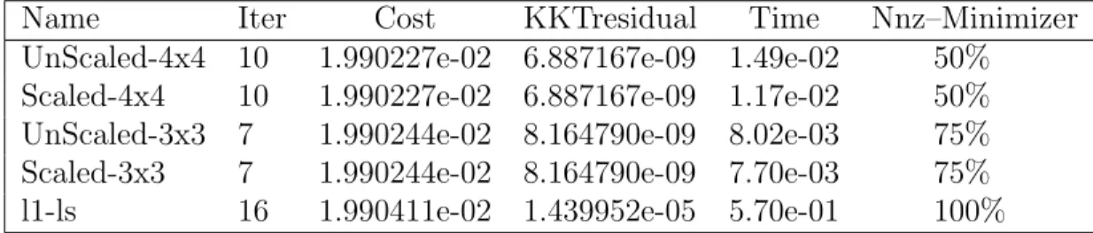
Table 5.1 A simple example of ℓ1− ℓs . . . 46
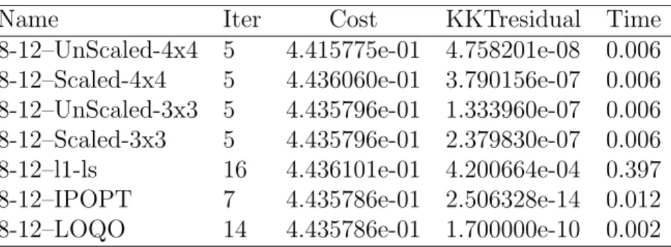
Table 5.2 Comparison for problem with p = 8 and n = 12 . . . . 48
Table 5.3 Comparison for problem with p = 32 and n = 8 . . . . 48
Table 5.4 Comparison for problem with p = 16 and n = 24 . . . . 48
Table 5.5 Comparison for problem with p = 64 and n = 16 . . . . 49
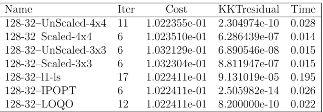
Table 5.6 Comparison for problem with p = 128 and n = 32 . . . . 49
Table 5.7 Comparison for problem with p = 256 and n = 64 . . . . 49
Table 5.8 Comparison for problem with p = 1024 and n = 256 . . . . 50
Table 5.9 Comparison for problem with p = 1072 and n = 768 . . . . 50
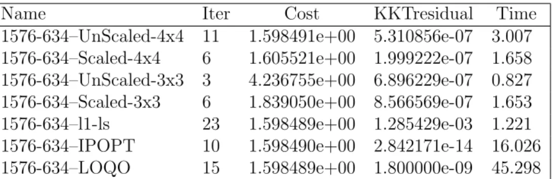
Table 5.10 Comparison for problem with p = 1576 and n = 634 . . . . 50
Table 5.11 Comparison for problem with p = 2048 and n = 512 . . . . 51
Table 5.12 Comparison for problem with p = 2144 and n = 1536 . . . . 51
Table 5.13 Comparison for problem with p = 1536 and n = 1072 . . . . 51
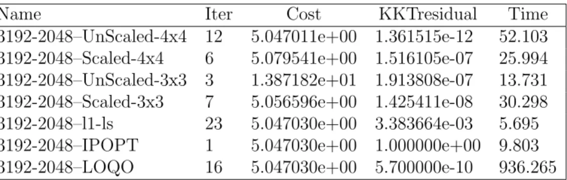
Table 5.14 Comparison for problem with p = 3192 and n = 2048 . . . . 52
Table 5.15 Comparison for problem with p = 1536 and n = 2192 . . . . 52
Table 5.16 Comparison for problem with p = 4096 and n = 1024 . . . . 52
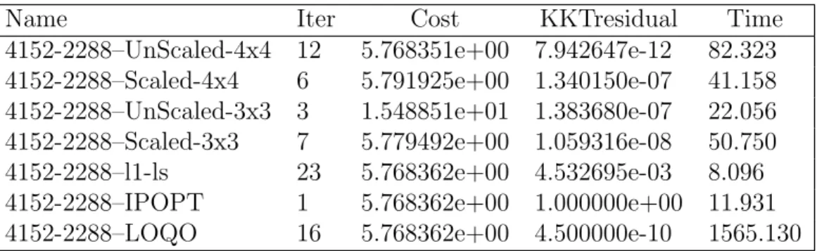
Table 5.17 Comparison for problem with p = 4152 and n = 2288 . . . . 53
LIST OF FIGURES
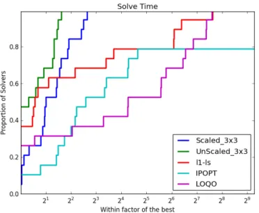
Figure 5.1 Performance in Terms of Time Using 3x3 . . . 54
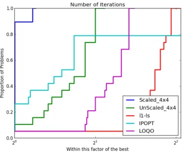
Figure 5.2 Performance in Terms of Number of Iterations Using 3x3 . . . 54
Figure 5.3 Performance in Terms of Time Using 4x4 . . . 55
LIST OF ACRONYMS AND ABBREVIATIONS
LS Least-Squares
DEM Direct Elimination Method NLS Non-Linear Least-Squares SQD Symmetric Quasi-Definite QP Quadratic Program(ing) LP Linear Program(ing)
SVD Singular Value Decomposition KKT Karush-Kuhn-Tucker
CG Conjugate Gradient Method
LSQR Sparse Equations and Least Squares
CGNE Conjugate Gradient Method On the Normal Equations CGLS Conjugate Gradient Method On the Least-Squares NMF Non-negative Matrix Factorization
LIST OF APPENDICES
ANNEXE A : IMPLEMENTATION . . . 67
ANNEXE B : NUMERICAL ALGEBRA REVIEW . . . 69
ANNEXE C : THE APPROXIMATE MINIMUM DEGREE (AMD) . . . 70
ANNEXE D : SQD MATRIX AND LDLT FACTORIZATION . . . . 71
CHAPTER 1
INTRODUCTION
We are concerned with the constrained linear least-squares problem in standard form minimize
x∈Rn c
Tx +1
2∥Ax − d∥
2 subject to Bx = b, x≥ 0, (1.1)
where c ∈ Rn, A ∈ Rp×n, d ∈ Rp, B ∈ Rm×n, b ∈ Rm and inequalities are understood componentwise. It is typically assumed that p > n and m < n but the approach proposed in this document allows us to do away with these restrictions. If A = 0, (1.1) reduces to the linear programming problem in standard form. In all other cases, (1.1) is a convex quadratic program. An interior-point method applied directly to (1.1) might suffer several difficulties. Firstly, the matrix ATA, which may be rather dense, will appear explicitly in the Newton step computation. Secondly, numerical instabilities will arise if the constraint matrix B does not have full row rank. We remove the first difficulty in two different ways that lead to two slightly different implementations. The second difficulty disappears by considering the following regularization of (1.1) proposed by Friedlander and Orban (2012):
minimize x∈Rn,w∈Rm c Tx + 1 2∥Ax − d∥ 2+ 1 2ρ∥x − xk∥ 2+ 1 2δ∥w + yk∥ 2 subject to Bx + δw = b, x≥ 0, (1.2)
where ρ > 0 and δ > 0 are regularization parameters, xk and yk are the current approxi-mations of the optimal primal variables and Lagrange multipliers, respectively, and w are auxiliary variables playing the role of a constraint residual. In this document, we specialize the interior-point framework of Friedlander and Orban (2012) and apply it to (1.2) with ulti-mately constant regularization parameters. At each iteration, a step is computed by solving a large and sparse symmetric quasi-definite linear system (Vanderbei, 1995). Contrary to most interior-point implementations, partial block elimination is not applied to this system to reduce it to the so-called augmented system form or to the normal equations. Instead, a similarity transformation is applied that guarantees that the system remains uniformly bounded and nonsingular throughout the iterations and in the limit provided strict comple-mentarity is satisfied at a solution. We establish global convergence under weak assumptions. In particular, no assumption on the rank of B or A is made. A distinctive feature of the regularization (1.2) is that it allows to recover a solution of (1.1) in many situations and
not only a solution of a perturbed problem. In addition, (1.2) is never solved to optimality for fixed values of ρ, δ, xk and yk. Instead, it is used to compute a single Newton step be-fore attention turns to the next regularized subproblem. In (1.2), the primal regularization term 12ρ∥x − xk∥2 serves the dual purpose of regularizing A whenever it is rank deficient and simplifying the implementation of the interior-point method in the presence of free vari-ables. The dual regularization term 12δ∥w + yk∥2 regularizes B whenever it is rank deficient.
The implementation proposed below relies on a sparse LDLT factorization of the symmetric quasi-definite coefficient matrix. This factorization may be obtained at lower cost than the symmetric indefinite factorization, such as that of Duff (2004), and typically yields sparser factors. Its stability on symmetric quasi-definite systems has been analyzed by Gill et al. (1996). Many applications only provide A and B in the form of linear operators instead of ex-plicit matrices. Iterative methods specialized to symmetric quasi-definite systems have been recently proposed by Arioli and Orban (2012). Our algorithm paves to way to a matrix-free implementation using such iterative methods. This yields an elegant framework in which an unconstrained regularized linear least-squares problem must be solved at each iteration. Our analysis and implementation differ from those of Friedlander and Orban (2012) in several respects. Firstly, the linear systems used in the definition of the Newton steps are larger, sparser and tailored to the special structure of (1.1). If strict complementarity holds at a solution, they also have uniformly bounded condition number. Secondly, our approach illustrates how to apply the primal-dual regularization of Friedlander and Orban (2012) se-lectively, leaving some variables and some constraints untouched. This has the benefit of exploiting the structure of the problem at hand.
1.0.1 Notation
The notation X and Z is used to denote the diagonal matrices diag(x) and diag(z). The vector e denotes the vector of all ones of appropriate dimension. The notation∥·∥ denotes the Euclidian norm throughout. The i-th component of a vector x is denoted [x]i while the value of x at the k-th iteration of a process is denoted xk. For a given positive definite matrix M , the M -norm is defined as ∥x∥2M = xTM x. The notation blkdiag(A1, . . . , Ak) denotes a block-diagonal matrix having the blocks A1 through Ak consecutively on the diagonal. Whenever a block Aj is an identity block, its size is dictated by the context. For two related sequences {αk} and {βk} of positive numbers, we write αk = O(βk) if there exists a constant C > 0 such that αk ≤ Cβk for all sufficiently large k. We write αk = Θ(βk) if αk = O(βk) and βk = O(αk).
CHAPTER 2
LITERATURE REVIEW
Carl Friedrich Gauss is credited with developing the fundamentals of the basis for least-squares (LS) analysis in 1795 at the age of eighteen. Gauss’s method came to be on January 1, 1801. The modern approach was first exposed in 1805 by the French mathematician Legendre Levenberg (1944). Nowadays, the LS method is widely used to find or estimate the numerical values of parameters to fit a function to a set of data. In this thesis, we are concerned with constrained and unconstrained linear least-squares problems. The second is the (Un)constrained Non-Linear Least-Squares method (NLS). We shall explain the NLS problem in a future section. There are essentially three different families of algorithms for solving a unconstrained linear-least square problem:
1. methods based on the normal equations; 2. methods based on the QR factorization;
3. methods based on the singular-value decomposition (SVD).
The first approach is the fastest and the most sensitive to ill conditioning. On the other hand, SVD is the most expensive and most accurate. Using the QR factorization to solve LS is numerically stable. An overview of those families of methods is provided in the following sections.
2.1 Factorization
The matrix factorization is a very useful linear algebra transformation, which targets the presentation of a matrix A as an appropriate product of matrices. There are many different matrix decompositions. Each finds use among a particular class of problems. Here we introduce a summary of the important matrix factorizations.
2.1.1 QR Factorization
The QR factorization decomposes the matrix A∈ Rm×n as
A = QR, (2.1)
where R is upper triangular and Q is orthogonal, i.e., QTQ = I. Such a decomposition can be performed both for a square matrix A with dimensions n× n, as well as more general
rectangular A with dimensions m× n. To solve the linear system of equations Ax = b, firstly the vector QTb = bQ is evaluated and then the triangular linear system Rx = bQ is solved. Due to the upper triangular form of R, this system of linear equations is easily solved by back substitution. The standard algorithm for the QR decomposition involves a sequence of Householder transformations. In the following sections, we provide more details about the answers to the following questions:
1. Does the QR factorization always exist? 2. Is this factorization unique?
3. Which Algorithms perform the QR factorization?
4. How is the QR factorization useful for solving linear least-squares problems? 5. What codes are available to perform the QR factorization?
2.1.1.1 Existence of the QR Factorization
For every matrix A, a QR factorization exists, even if A does not have full rank. The existence of this factorization follows from Householder transformations. One can prove the following two theorems related to the QR factorization of a matrix A.
Theorem 2.1.1. Every matrix A possesses a QR factorization.
Theorem 2.1.2. (Full QR Factorization)(Trefethen and Bau (1997)[Theorem 5.1]) Let A be a non-singular matrix. There exists a unique pair (Q, R), where Q is an orthogonal matrix and R is an upper triangular matrix, whose diagonal entries are real, satisfying A = QR.
The overall complexity (number of oating points) of the QR factorization is n3
2.1.1.2 Forms of the QR Factorization – If A has full rank
1. If A is square, R has the form
Rn,n= ⋆ ⋆ · · · ⋆ 0 ⋆ · · · ⋆ .. . ... . .. ... 0 0 · · · ⋆ .
If A is non-square, R is non-square too,
2. If A has more columns than rows, i.e., n > m we can write R = [
R1 | R2 ] where R1 is upper triangular.
3. The most common case encountered in linear least-squares problems is where A is m× n, with m > n. In this case we have R =
[ R1 0 ] where R1 is n× n triangular, and Q = [ Q1 | Q2 ] A = [ Q1 | Q2 ] [R 1 0 ] = Q1R1+ Q20 = Q1R1,
where Q1 is an m× n matrix whose columns are orthogonal. – If A does have not full rank
In this case R has the form
R = ⋆ ⋆ · · · ⋆ ⋆ · · · ⋆ . .. ...
0
⋆ 0 0 0 0 .It is often of interest to discover the rank of A. Given a decomposition of the form (2.1), rank(A) = rank(R), and in practice, this QR decomposition is a good way to determine the rank of a matrix. The computations are quite sensitive to rounding, however, and therefore it must be done with some care. If columns of A are linearly independent, then this factorization is unique. There are many practical algorithms in Golub and Van Loan (1996).
2.1.1.3 Codes Available to Perform the QR Factorization
1. BAND–QR is a FORTRAN90 library which includes LAPACK–style routines to com-pute the QR factorization of a banded matrix.
2. From python using the scipy package, we can use scipy.linalg.qr. 3. Using qr from Matlab.
2.1.2 SVD
The Singular Value Decomposition (SVD) of a matrix A takes the form, A = U ΣV,
where U and V are orthogonal and Σ is a diagonal positive semidefinite matrix.
Theorem 2.1.3. (The Singular Value Decomposition Theorem ) Let A be a real m× n matrix. Then there exist orthogonal matrices U and V such that
UTAV = [ Σ1 0 0 0 ] = Σ,
where Σ1 is a nonsingular diagonal matrix. The diagonal entries of Σ are all nonnegative and can be arranged in a non increasing order. The number of nonzero diagonal entries of Σ equals the rank of A.(Datta (2010)[Theorem 10.2.1])
The SV D of a matrix A is typically computed by a two-step procedure. In the first step, the matrix is reduced to a bidiagonal matrix. This takes O(mn2) floating-point operations
(flops), assuming that m≥ n (this formulation uses the big O notation). The second step is to compute the SV D of the bidiagonal matrix. This step can only be done with an iterative method (as with eigenvalue algorithms Trefethen and Bau III 1997, Lecture 31).
2.1.3 Cholesky Factorization
Theorem 2.1.4. (The Cholesky Factorization Theorem ) If A is symmetric and positive definite, then A can be decomposed as
A = LLT
where L is a lower triangular matrix with strictly positive diagonal entries. (Trefethen and Bau (1997)[Theorem 32.1.])
2.1.4 SQD Matrix and LDLT Factorization
A symmetric matrix is called quasidefinite if it can be written, perhaps after a symmetric
permutation, as [
−E A AT D ]
,
where E and D are symmetric and positive definite matrices. The LDLT factorization can be used on this kind of matrix. The following theorem states a nice feature of SQD matrices. This property can be used to have a sparse L in the LDLT factorization of a SQD matrix.
Theorem 2.1.5. Any symmetric permutation P of a SQD matrix K possesses a factor-ization P KPT = LDLT, where L is unit lower triangular and D is diagonal. (Vanderbei (1995)[Theorem 12])
2.2 Unconstrained Linear Least-Squares Problems
Suppose A∈ Rp×n, p≥ n, d ∈ Rp are given. We can write the residual vector as r(x) = Ax− d for x ∈ Rn.
The linear least-squares problem is defined as the following optimization problem min
x∈Rnf (x), (2.2)
where f (x) = 12∥r(x)∥2 = 1
2∥Ax − d∥
2. By definition of f (x) the gradient and the Hessian
of f (x) are ∇f(x) = AT(Ax− d) and ∇2f (x) = ATA. Since xTATAx = ∥Ax∥2 ≥ 0 for
any x ∈ Rn, ∇2f (x) is positive semi-definite. Therefore, f (x) is convex and any point x∗ for which ∇f(x∗) = 0 is a global minimizer of f . Therefore a solution, x∗ must satisfy the following linear system of equations:
ATAx∗ = ATd. (2.3)
In other words, since∇2f (x) is positive semi-definite,∇f(x) = 0 are not only necessary but
2.2.0.1 Using the QR Factorization to Solve LS
The Householder implementation of the QR factorization requires 2mn2−2 3n
3 flops. The
Euclidean norm of any vector is not affected by orthogonal transformations. Therefore, we have
∥Ax − d∥ = ∥QT(Ax− d)∥, (2.4)
for any m× m orthogonal matrix Q. Suppose we perform a QR factorization on matrix A, so that A = [ Q1 Q2 ] [R 1 0 ] = Q1R1, (2.5)
where Q1 is n× n, Q2 is (m− n) × n and R1 is n× n. From (2.4) and (2.5) we have ∥Ax − d∥2 = [ QT1 QT 2 ] (Ax− d) 2 = [ QT 1 QT 2 ] ([ Q1 Q2 ] [R 1 0 ] x− d ) 2 = [ R1 0 ] x− [ QT 1d QT 2d ] 2 = [ R1x− QT1d 0− QT2d ] =∥R1x− QT1d∥2+∥QT2d∥2
The second term of the last expression is not dependent on x. If we want to minimize (2.2), the optimal solution is equal to
x∗ = R−11 QT1d, and the optimal objective value is ∥QT
2d∥. In summary, we can use the following procedure
1. Compute the reduced QR factorization A = QR. 2. Compute the vector QTd.
3. Solve the upper-triangular system Rx = QTd for x. Fore more information, see (Nocedal and Wright (1999)[ 10.2]).
2.2.0.2 Using the Cholesky Factorization to Solve LS
The classical way to solve least-squares problems is to solve the normal Equation (2.3). The standard method of solving (2.3) is to use the Cholesky factorization, ATA = LLT where L is lower-triangular, reducing (2.3) to
LLTx = ATd. (2.6)
Now consider the factorization A = QR, then ATA = RTR. The uniqueness of the Cholesky factors then implies that R = LT. In summary, we can use the following procedure:
1. Compute the coefficient matrix ATA and the right-hand-side ATd.
2. Compute the Cholesky factorization of the symmetric matrix ATA = LLT = RTR. 3. Solve the lower-triangular system Ly = ATd for y.
4. Solve the upper-triangular system LTx = y for x.
Computing ATA requires mn2 flops and the Cholesky factorization requires n63 flops. All together, solving least-squares problems by the normal equations involve mn2+16n3 flops. If m ≫ n this method is twice as fast as the QR factorization.
2.2.0.3 Using the SVD Factorization to Solve LS Let A = U ΣVT be the SV D of A. Then we have
∥Ax − d∥2 =∥UΣVTx− d∥2
=∥U(ΣVTx− UTd)∥2 =∥Σy − d′∥2
where VTx = y and UTd = d′. Thus, the use of SV D of A reduces the least-squares problem for a full matrix A to one with a diagonal matrix Σ. Now we need to solve the following trivial optimization problem (Datta (2010)[ 10.2]).
minimize
y ∥Σy − d
′∥.
2.2.1 Iterative Methods to Solve LS
Linear least-squares problems can also be solved using iterative methods that generally fall into the category of Krylov methods Bjorck (1996). We give a brief overview of such methods in the rest of this section.
2.2.1.1 Conjugate Gradient Method on the Normal Equations (CGNE)
The conjugate gradient method can be applied to an arbitrary system Ax = d by applying it to the normal equations matrix ATA and right-hand side vector ATd, since ATA is a sym-metric positive-semidefinite matrix for any A. The result is the conjugate gradient method on the normal equations (CGNE). As an iterative method, it is not necessary to form ATA explicitly in memory; rather, only to perform matrix-vector and transpose matrix-vector multiplications. Therefore (CGNE) is particularly useful when A is a large sparse matrix since these operations are usually extremely efficient. However, the downside of forming the normal equations is that the condition number Cond(ATA) is equal to Cond2(A) and so the rate of convergence of (CGNE) may be slow and the quality of the approximate solution may be sensitive to roundoff errors. Finding a good preconditioner is often an important part of using the (CGNE) method. Several algorithms have been proposed (e.g., CGLS, LSQR). The LSQR algorithm purportedly has the best numerical stability when A is ill-conditioned, i.e., A has a large condition number (Lawson and Hanson (1995)[ 20]).
2.2.1.2 LSQR
LSQR is an algorithm for solving sparse least-squares problems. Consider the following regularized problem minimize x 1 2 [ A λI ] x− [ d 0 ] 2 (2.7) where A and d are given data and λ is an arbitrary real scalar. The matrix A may be square or rectangular over-determined or under-determined, and may have any rank. The solution of (2.7) satisfies the symmetric quasi-definite system
[ I A AT −λ2I ] [ r x ] = [ d 0 ] ,
where r is the residual vector d−Ax. Paige and Saunders (1982) use an iterative method based on the bidiagonalization procedure of Golub and Kahan. LSQR is algebraically equivalent to applying CG to the normal equations (ATA)x = ATd, but has better numerical properties, especially if A is ill-conditioned (Paige and Saunders (1982)).
2.3 Constrained Linear Least-Squares Problems
In terms of linear least-squares with linear equality constraints, we have the following base methods. One could consider the LS problem as
minimize x c Tx + 1 2∥Ax − d∥ 2 subject to Bx = b, x≥ 0. (2.8) Background and suggestions for further reading can be found in the seminal book of Hanson and Lawson (1969), who have described three methods for solving (2.8) as follows:
1. methods based on the null space; 2. methods based on direct elimination; 3. methods based on weighted LS.
2.4 Regularization
In this thesis, we consider a primal-dual regularization of convex QPs which specializes the interior-point framework of Friedlander and Orban (2012). Consider the convex quadratic program (QP) minimize x c Tx +1 2x TQx subject to Ax = b, x≥ 0. (2.9) Now consider the regularization
minimize x,r c Tx +1 2x TQx +1 2ρ∥x − xk∥ 2+ 1 2δ∥r + yk∥ 2 subject to Ax + δr = b, x≥ 0, (2.10) of (2.9), where ρ > 0 and δ > 0 are regularization parameters, and xk and yk are current estimates of primal and dual solutions. The strength of the approach is that the dual of (2.10) is the regularization of the dual of (2.9). It is easy to see that a constrained linear
least-squares problem is a special case of convex QP. Indeed, consider the following constrained linear least-squares problem
minimize
x∈Rn c
Tx +1
2∥Ax − d∥
2 subject to Bx = b, x≥ 0. (2.11)
It is equivalent to the following convex QP: minimize x,r c Tx + 1 2∥r∥ 2 subject to Bx = b, Ax + r = d, x≥ 0. (2.12)
CHAPTER 3
A VARIANT OF THE METHOD OF FRIEDLANDER AND ORBAN (2012)
In this chapter we are going to specialize an infeasible regularized interior-point algo-rithm called primal-dual for constrained linear least-squares problems (2.8) based on the primal-dual regularization of convex programs (2.9) of Friedlander and Orban (2012). Our approach illustrates how to apply the primal-dual regularization of Friedlander and Orban (2012) selectively, leaving some variables and some constraints untouched.
3.0.1 Regularization in the Primal-Dual Interior-Point Method Consider the regularized form of (2.11)
minimize x,w c Tx +1 2∥Ax − d∥ 2+ 1 2ρ∥x − xk∥ 2+1 2δ∥w + yk∥ 2 subject to Bx + δw = b, x≥ 0, (3.1)
proposed by Friedlander and Orban (2012) where ρ > 0 and δ > 0 are regularization parame-ters, and xk and yk are current estimates of primal and dual solutions. The original problem (2.11) can be recovered by considering ρ = 0 and δ = 0. The dual is given by
maximize x,y,s,z b Ty− (ATd)Tx−1 2∥Ax − d∥ 2−1 2δ∥y − yk∥ 2− 1 2ρ∥s + xk∥ 2 (3.2) subject to BTy + z− ATAx = c− ATd, z≥ 0,
where{y, z} are Lagrange multipliers corresponding to the equalities and bound constraints of (2.11) and s = x− xk are auxiliary variables.
An interior-point method places the slacks in a barrier term, leading to the following primal-dual pair in which µ > 0 is a barrier parameter:
minimize x,w c Tx +1 2∥Ax − d∥ 2+1 2ρ∥x − xk∥ 2+1 2δ∥w + yk∥ 2− µk n ∑ i=1 ln xi subject to Bx + δw = b, (3.3)
maximize x,y,s,z b Ty− (ATd)Tx−1 2∥Ax − d∥ 2−1 2δ∥y − yk∥ 2− 1 2ρ∥s + xk∥ 2− µk n ∑ i=1 ln zi subject to BTy + z− ATAx = c− ATd. (3.4) 3.0.2 Newton System
Let (xk, yk) be temporarily fixed. A primal-dual interior point method applied to the regularized problems (3.3) and (3.4) is based on applying a single Newton iteration to a sequence of non-linear equations of the form
ωk(v; ρ, δ, µk) := c + ρs− ATr− BTy− z Ax + r− d ρx− ρ(s + xk) δy− δ(w + yk) Bx + δw− b Xz− σµke = 0, (x, z)≥ 0, (3.5)
where v = (x, r, s, w, y, z), µk > 0 is the current duality measure, which is equal to xTkzk/n, and σ ∈ [0, 1] is a centring parameter. For fixed ρk, δk, xk, and yk the central path is the exact solution of (3.5) with σ = 1 (Wright, 1997). As µk → 0, it can be illustrated that this central path leads to a primal-dual solution to (3.3) and (3.4). Since objective function and constraints are convex, the necessary and sufficient optimality conditions can be written more succinctly as
ω(v; 0, 0, 0) = 0, and (x, z)≥ 0.
A Newton step for (3.5) from the current iterate ωk is based on solving the system
0 −AT ρI 0 −BT −I
A I 0 0 0 0 ρI 0 −ρI 0 0 0 0 0 0 −δI δI 0 B 0 0 δI 0 0 Z 0 0 0 0 X ∆x ∆r ∆s ∆w ∆y ∆z =− c + ρs− ATr− BTy− z Ax + r− d ρx− ρ(s + xk) δy− δ(w + yk) Bx + δw− b Xz− σµe . (3.6)
The block matrix in (3.6) can be reduced by eliminating the variables ∆w and ∆s: −ρI AT BT I A I 0 0 B 0 δI 0 Z 0 0 X ∆x ∆r ∆y ∆z = c− ATr− BTy− z d− Ax − r b− Bx XZ − σµe . (3.7)
The remaining directions may be recovered via
∆w = ∆y− wk, ∆s = ∆x− sk. (3.8)
By eliminating the variable ∆z from (3.7) we arrive at −(X−1Z + ρI) AT BT A I 0 B 0 δI ∆x ∆r ∆y = c− ATr− BTy− σµX−1e d− Ax − r b− Bx , (3.9)
where the variable ∆z is recovered via
∆z =−z − X−1Z∆x + σµX−1e. (3.10)
The system (3.9) will be discussed further in this chapter. Note that upon setting ρ = δ = 0, we recover the Newton equations used to compute a step from the k-th iterate of an interior-point method applied to (3.1)–(3.2). As shown in (3.9) we take x = xk, r = rk, and y = yk at each iteration. More precisely, the central path C is an arc of strictly feasible points defined as the solutions of Bx + δw− b = 0 (3.11a) Ax + r− d = 0 (3.11b) c− ATr + ρs− BTy− z = 0 (3.11c) δy− δ(w + yk) = 0 (3.11d) ρx− ρ(s + xk) = 0 (3.11e) Xz = µe (3.11f) (x, z) > 0, (3.11g)
for positive values of µ. If (xµ, rµ, sµ, wµ, yµ, zµ) solves (3.11) then the central path is the set C = {(xµ, rµ, sµ, wµ, yµ, zµ) | µ > 0}.
It can be shown that (xµ, rµ, sµ, wµ, yµ, zµ) is defined uniquely for any µ > 0 if and only if C is non-empty (Wright, 1997, Theorem 2.8).
3.0.3 Nk Neighbourhood
A difference between our approach and traditional interior-point methods is that during the course of the iterations, the regularization parameters ρ and δ may be updated. At the k-th iteration, the current iterate is vk := (xk, rk, sk, wk, yk, zk) and the regularization parameters have values ρk and δk. We consider a neighbourhood Nk of the central path as the set of points (x, r, s, w, y, z) that satisfy the following conditions:
¯ γCxTz/n≥ [x]i[z]i ≥ γCxTz/n, (3.12a) xTz ≥ γP∥Bx + δkw− b∥, (3.12b) xTz ≥ γR∥Ax + r − d∥, (3.12c) xTz ≥ γD∥c + ρks− BTy− ATr− z∥, (3.12d) xTz ≥ γS∥ρkx− ρk(s + xk)∥, (3.12e) xTz ≥ γW∥δky− δk(w + yk)∥, (3.12f) where 0 < γC < 1 < γC and (γP, γD, γR, γS, γW) > 0 are given constants. Our interior-point scheme generates the new iterate vk+1 as follows:
vk(αk) := (xk+ αk∆x, rk+ αk∆r, sk+ αk∆s, wk+ αk∆w, yk+ αk∆y, zk+ αk∆z), where αk ∈ (0, 1] and (∆x, ∆r, ∆s, ∆w, ∆y, ∆z) is computed via (3.9), (3.8), and (3.10).
3.0.4 Algorithm
Our algorithm is the same as (Friedlander and Orban, 2012, Algorithm 4.1) with the exception of the linear system used in Step 2, and is formalized as Algorithm 3.0.1.
Algorithm 3.0.1 Primal-Dual Regularized Interior-Point Algorithm
Step 0 [Initialize] Choose minimum and maximum centering parameters 0 < σmin ≤ σmax < 1, a constant σmax < β < 1, proximity parameters 0 < γC < 1 < ¯γC and (γP, γR, γD, γS, γW) > 0, initial regularization parameters ρ0 > 0, δ0 > 0, and a
stop-ping tolerance ϵ > 0. Let the neighborhood of the central path be defined by (3.12a), (3.12b), (3.12c) and (3.12d). Choose initial primal x0 ∈ Rn
++, r0 ∈ Rm, w0 ∈ Rm and
dual guesses s0 ∈ Rn, y0 ∈ Rm, and z0 ∈ R++n so that v0 ∈ N0. Set µ0 := xT0z0/n and
k = 0.
Step 1 [Test convergence ] If xT
kzk ≤ ϵ, declare convergence.
Step 2 [Step computation] Choose a centering parameter σk∈ [σmin, σmax]. Compute the Newton step ∆vk from vk, e.g., by solving (3.9) with and recovering the remaining components from (3.8) and (3.10).
Step 3 [Linesearch] Select δk+1 ∈ (0, δk] and ρk+1 ∈ (0, ρk] and compute αk as the largest α∈ (0, 1] such that
vk(α)∈ Nk+1 and µk(α)≤ (1 − α(1 − β))µk, (3.13) where µk(α) := xk(α)Tz
k(α)/n.
Step 4 [Update iterates] Set vk+1 := vk(αk), µk+1:= µk(αk). Increment k by 1 and go to Step 1.
3.1 Global Convergence Analysis
We begin our analysis by providing bounds on the eigenvalues of the matrix
Kk := [ −Hk A˜T ˜ A Iδ k ] , (3.14) where Hk= (Xk−1Zk+ ρkI), A =˜ [ A B ] , and Iδ k = [ I 0 0 δkI ] .
The block matrix Kk in (3.14) is the matrix that appears in Step 2 of Algorithm 3.0.1. In the remainder of this section, we simplify the notation by dropping the iteration counter k.
The inertia of a symmetric matrix K is the triple of non-negative integers (n+, n−, n0), where n−, n0, and n+ are the number of negative, zero, and positive eigenvalues of K,
respectively. The following lemma states the relation between the inertia of matrix K and that of BTKB where B ∈ Rn×n is nonsingular.
Lemma 3.1.1. (Sylvester’s Law of Inertia) If K ∈ Rn×n is symmetric and B ∈ Rn×n is nonsingular, then K and BTKB have the same inertia.
Proof. See (Golub and Van Loan, 1996, Theorem 8.1.17). The eigenvalue bounds
λmin(H)≥ λmin( ˜A) + min
1≤i≤n
[z]i [x]i
+ ρ and λmax(H)≤ λmax( ˜A) + max
1≤i≤n
[z]i [x]i
+ ρ, (3.15)
and the congruence relation [ −H ˜AT ˜ A Iδ ] = [ I 0 − ˜AH−1 I ] [ −H 0 0 AH˜ −1A˜T + I δ ] [ I −H−1A˜T 0 I ] (3.16)
are useful for the next theorem, which is a variant of (Friedlander and Orban, 2012, Theo-rem 5.1) for least-squares problems.
Theorem 3.1.2. For all (x, z) > 0 and all ρ > 0 and δ > 0, K possesses precisely n negative eigenvalues and m + n positive eigenvalues. Let them be denoted and ordered as
−λ−n ≤ λ−n+1≤ · · · ≤ λ−1 < 0 < λ1 ≤ · · · ≤ λm+n−1 ≤ λn+m.
The largest positive and smallest negative eigenvalues of K satisfy the bounds λ−n≥ 1 2[δ− λmax(H)]− 1 2[(λmax(H)− δ) 2+ 4(σ max( ˜A)2+ λmax(H)δ)] 1 2, (3.17a) λn+m ≤ 1 2[δ− λmin(H)] + 1 2[(λmin(H)− δ) 2 + 4(σ min( ˜A)2+ λmin(H)δ)] 1 2. (3.17b)
The smallest positive and largest negative eigenvalues of K satisfy the bounds
λ−1 ≤ −λmin(H), (3.17c) λ1 ≥ 1 2[δ + λmax(H)]− 1 2[(λmax(H)− δ) 2 + 4(σmin( ˜A)2+ λmax(H)δ)] 1 2. (3.17d)
Moreover, λ1 = ˜δ where ˜δ = min(1, δ) is the smallest positive eigenvalue of K if and only if ˜A does not have full row rank. In this case, its associated eigenspace is {0} × Null( ˜AT). Its geometric multiplicity is thus m+n-rank( ˜A).
Proof. The first part of the theorem follows from (3.16) and Sylvester’s law of inertia. Note that H and ˜AH−1A˜T + I
δ are positive definite because of the positivity assumption on x, z, ρ, and δ. The rest of the proof parallels (Silvester and Wathen, 1994, Lemma 2.2).
If (u, v)̸= 0 is an eigenvector of K associated to the eigenvalue λ, then
−Hu + ˜ATv = λu (3.18a)
˜
Au + Iδv = λv. (3.18b)
Note that λ = 1 is an eigenvalue of K if and only if A does not have full row rank, and its associated eigenspace is {0} × Null(AT), similarly, λ = δ is an eigenvalue of K if and only if B does not have full row rank, and its associated eigenspace is {0} × {0} × Null(BT) Now, suppose λ ̸= δ and λ ̸= 1. From (3.18b), we have v = (λI − Iδ)−1Au. Necessarily, u˜ ̸= 0. Substituting into (3.18a) and taking the inner product with u yields
λ∥u∥2 =−uTHu + (λI − Iδ)−1uTA˜TAu.˜ (3.19) If λ < ˜δ, then, because the right-hand side of (3.19) is negative, we must have λ < 0, and
so λ1 ≥ δ. But by the implication drawn from (3.18), λ1 = δ if and only if ˜A is rank deficient. This proves the last statement of the theorem.
If λ > ˜δ, we deduce from (3.19) that
λ∥u∥2 ≤ −λmin(H)∥u∥2+ (λ− ˜δ)−1σmax( ˜A)2∥u∥2.
Upon simplifying and substituting ℓ for λ, we see that the quadratic ℓ2+ (λmin(H)− ˜δ)ℓ − (σmax(B)2+ λmin(H)˜δ)
in ℓ takes a nonpositive value when evaluated at an eigenvalue λ > δ of K. In particular this must be true of λm, which yields (3.17b).
If λ < 0, (3.19) yields the bound
λ∥u∥2 ≥ −λmax(H)∥u∥2+ (λ− max(1, δ))−1σmax( ˜A)2∥u∥2. In turn, this implies that the quadratic in ℓ,
ℓ2 + (λmax(H)− ˜δ)ℓ − (σmax(B)2+ λmax(H)˜δ),
takes a nonpositive value when evaluated at an eigenvalue λ < 0 of K. In particular this must be true of λn < 0, which yields (3.17a). We now establish (3.17a). we have two cases for λ
1. If λ < 0 by multiplying uT and vT to left hand side of (3.18a) and (3.18a) respectively we have
−uTHu + uTA˜Tv = λ∥u∥2, (3.20)
vTA˜Tu + vTIδv = λ∥v∥2. (3.21) By subtracting (3.20) from (3.21) we obtain
−uTHu− vTI
δv = λ(∥u∥2− ∥v∥2). (3.22) Since we have
−uTHu≤ −λ
min(H)∥u∥2 ≤ −ρ∥u∥2,
−vTI
δv ≤ −˜δ∥v∥2, from (3.22) we get
Therefore, the following inequality is obtained
(λ + ρ)∥u∥2 ≤ (λ − ˜δ)∥v∥2 ≤ 0. So necessarily u must be nonzero and we have
λ−1 ≤ −ρ.
2. If λ > 0 using u = (H + λI)−1A˜Tv from (3.20) and substituting in (3.21) we get ˜
A (H + λI)−1A˜Tv + Iδv = λv, by multiplying vT from left we have that
vTA (H + λI)˜ −1A˜Tv + vTIδv = λ∥v∥2. (3.23) Since vTA (H + λI)˜ −1A˜Tv ≥ λmin ( ˜ A(H + λI)−1A˜T ) ∥v∥2 ≥ λmin ( ˜ A ˜AT ) λmin((H + λI)−1)∥v∥2 ≥ σmin( ˜A)2 1 λmax(H) + λ∥v∥ 2
and vTIδv ≥ ˜δ∥v∥2 from (3.23) we have that
λ∥v∥2 ≥ ( σmin( ˜A)2 λmax(H) + λ + ˜δ ) ∥v∥2 ≥ ˜δ∥v∥2 So we have λ > min(1, δ), and λ1 > ˜δ,
Corollary 3.1.3. For all (x, z) > 0 and ρ > 0 and δ > 0 the smallest positive and the largest negative eigenvalues of K satisfy
1. λ1 > ˜δ 2. λ−1 ≤ −ρ 3. ∥K∥−1 ≤ 1
min(ρ,˜δ)
Proof. Because ∥K∥−1 = max(λ−1
−1, 1 λ1), ∥K∥−1 ≤ max(1 ρ, 1 ˜ δ ) = 1 min(ρ, ˜δ).
Turning now to the right hand side of the Newton system (3.6), i.e.,
−Ax − r + d, (3.24a) −c + ATr + BTy− ρs + z, (3.24b) −ρx + ρ(s + xk), (3.24c) −δy + δ(w + yk), (3.24d) b− Bx − δw, (3.24e) XZ− σµe, (3.24f)
from (3.24a) we have
− A(x + α∆x) − (r + α∆r) + d = −Ax − r + d − α(A∆x + ∆r).
Since
∆r =−A∆x − Ax − r + d, (3.25)
(3.25) becomes
− Ax − r + d − α(−Ax − r + d) = (1 − α)(Ax − r + d).
From (3.24b) we have
− c + AT(r + α∆r) + BT(y + α∆y)− ρ(s + α∆s) + z + α∆z = − c + ATr + αAT∆r + BTy + αBT∆y− ρs − αρ∆s + z + α∆z = (−c + ATr + BTy− ρs + z) − α[−AT∆r− BT∆y + ρ∆s+
(−ρ∆s + AT∆r + BT∆y− c + ATr + BTy + z)], the last equality becomes
−α(−c + ATr + BTy− ρs + z)(1 − α)(−c + ATr + BTy− ρs + z). (3.27)
From (3.24c) we have
ρ(s + α∆s) = ρs + ρα∆x− ραs = (1 − α)ρs + ρα∆x, (3.28) and from (3.24d) we have
δ(w + α∆w) = δw + δα∆w = δw + δα(∆y− w) = (1 − α)δw + δα∆y. (3.29) From (3.24e) and δ∆w =−B∆x + b − Bx − δw we arrive at
b− B(x + α∆x) − δ(w + α∆w) = b − Bx − αB∆x − δw − αδ∆w = (1 − α)(b − Bx − δw). (3.30) From (3.24f) and the fact that Z∆x + X∆z =−Xz + σµe we have
zT∆x + xT∆z =−xTz + nσµ =−xTz + σxTz =−(1 − σ)xTz, (3.31) and zi[∆x]i+ xi[∆z]i =−xizi+ σx Tz n . (3.32) 3.1.1 Fixed Regularization
Our first method, described in Algorithm 3.1.1, holds the regularization parameters ρ and δ fixed at all iterations and enforces conditions (3.12a)-(3.12d) at each iteration. Since the regularization parameters are constant in this section, we simply denote them ρ and δ for readability. Convergence properties rely on the following technical lemma.
Algorithm 3.1.1 Variation of the primal–dual method with constant regularization
Apply Algorithm 3.0.1 with ρk := ρ0 > 0 and δk := δ0 > 0 for all k. In step 3, only conditions (3.12a)- (3.12d) are enforced.
Lemma 3.1.4. Suppose that (∆x, ∆r, ∆y, ∆z) is given by Step 2 of Algorithm 3.1.1, and the sequence {(sk, wk, zk)} is bounded. Then there exists a constant π, dependent only on n, such that
|[∆x]i[∆z]i| ≤ π, |[∆x]i[∆z]i− γC∆xT∆z/n| ≤ π, and |[∆x]i[∆z]i− ¯γC∆xT∆z/n| ≤ π.
Proof. The proof is similar to (Friedlander and Orban, 2012, Lemma 5.3). In order to prove the required result, it is sufficient to demonstrate that (∆x, ∆r, ∆y, ∆z) is bounded. To that end, we first show that (∆x, ∆r, ∆y) is bounded, and second show that ∆z is bounded. We have from (3.12b) and (3.13) that
∥Bxk− b∥ ≤ ∥Bxk+ δwk− b∥ + δ∥wk∥ ≤ xTzk/γP + δ sup k ∥wk∥, ≤ xT 0z0/γP + δ sup k ∥wk∥ ∥d − Axk− rk∥ ≤ xT kzk/γR≤ xT0z0/γR,
which shows that the second block of the right-hand side in (3.9) is bounded. We now show that the first block in (3.9) is bounded. It follows from (3.12a) that
σ ¯ γCz≤ σµX −1e≤ σ γCz, componentwise. As a consequence, ∥σkµkX−1e− zk∥ ≤ M sup k ∥zk∥, where M := max( σ γC − 1 , ¯γσC − 1 ) .
Combining this last inequality with (3.12d) and (3.13), we obtain ∥c − ATr
k− BTyk− σµX−1e∥ = ∥c − ATrk− BTyk− σµX−1e± ρsk± zk∥ ≤ xT
0z0T/γD+ ρ sup
k ∥sk∥ + M supk ∥zk∥.
bounded because the right-hand side of (3.9) is bounded. To show that ∆z is bounded, we note that ∆z satisfies (3.9), which has a bounded right-hand side.
Our convergence analysis rests upon a variation of (Friedlander and Orban, 2012, Theo-rem 5.4) stating the convergence properties of Algorithm 3.1.1. The next result implies that the duality measure µk converges to zero under a boundedness assumption.
Theorem 3.1.5. Suppose that Algorithm 3.1.1 with ϵ = 0 generates the sequence {vk}, and that the sequence {(sk, wk, zk)} is bounded. Then µk→ 0.
Proof. We follow Kojima et al. (1993), and express (3.13) in Step 3 of the algorithm as (fi(α)), ¯fi(α)≥ 0, h(α) ≥ 0, gP(α)≥ 0, gR(α)≥ 0, and gD(α)≥ 0, (3.33) for i = 1,· · · , n, where, dropping for the moment the subscript k,
fi(α) := ([x]i+ α[∆x]i)T([z]i+ α[∆z]i)− γC(x + α∆x)T(z + α∆z)/n, (3.34a) ¯ fi(α) := ¯γC(x + α∆x)T(z + α∆z)/n− ([x]i+ α[∆x]i)T([z]i+ α[∆z]i), (3.34b) h(α) := (1− α(1 − β))xTz− (x + α∆x)T(z + α∆z), (3.34c) gP(α) := (x + α∆x)T(z + α∆z)− γP∥B(x + α∆x) + δ(w + α∆w) − b∥, (3.34d) gR(α) := (x + α∆x)T(z + α∆z)− γR∥A(x + α∆x) + (r + α∆r − d)∥, (3.34e) gD(α) := (x + α∆x)T(z + α∆z)− γD∥c + ρ(s + α∆s) − BT(y + α∆y) (3.34f) − AT (r + α∆r)− (z + α∆z)∥, (3.34g)
and by contradiction, we assume that xTz ≥ ¯ϵ for some ¯ϵ > 0. We use (3.31) and (3.32) and Lemma 3.1.4, and the inequality xTz ≥ ¯ϵ to show that fi(α) ≥ 0, ¯fi(α) ≥ 0 and h(α) ≥ 0 . We establish a similar property for gP(α), gR(α), and gD(α). Using (3.30), (3.27), (3.31), and (3.34a) and the rest of proof is similar to (Friedlander and Orban, 2012, Theorem 5.4).
In the next chapter, we propose a variation of Algorithm 3.0.1 in which the linear system (3.9) differs. Partial block elimination is not applied and this results in a larger but sparser SQD system. The convergence analysis rests upon a variation on (Armand and Benoist, 2011, Theorem 1) stating that the inverse of the coefficient matrix of Newton system remains uniformly bounded as long as {xk} and {zk} remain bounded away from zero.
CHAPTER 4
A REGULARIZED INTERIOR-POINT METHOD FOR CONSTRAINED LINEAR LEAST SQUARES
4.1 Background and Preliminaries
As a convex quadratic program, the dual of (1.1) may be written as the constrained linear least-squares problem maximize x,y,z b Ty− (ATd)Tx− 1 2∥Ax − d∥ 2 subject to BTy + z− ATAx = c− ATd, z ≥ 0, (4.1)
where y ∈ Rm and z ∈ Rn are the vectors of Lagrange multipliers associated to the equality constraints and bounds of (1.1), respectively.
Friedlander and Orban (2012) justify the regularization (1.2) of (1.1) as an application of the proximal method of multipliers of Rockafellar (1976). It consists in the addition of a proximal-point term 12ρ∥x − xk∥2, to which we will refer as a primal regularization term,
and of augmented Lagrangian terms consisting of the objective term 12δ∥w + yk∥2 and the
constraint residual term δw, to which we will collectively refer as a dual regularization term. The regularized problem (1.2) is still a convex quadratic program and its dual may be written as the regularized constrained linear least-squares problem
maximize x,s,y,z b Ty− (ATd)Tx− 1 2∥Ax − d∥ 2− 1 2δ∥y − yk∥ 2− 1 2ρ∥s + xk∥ 2 subject to BTy + z− ATAx− ρs = c − ATd, z ≥ 0, (4.2)
where s = x− xk are auxiliary variables playing the same role as w in (1.2). The strength of this regularization approach is that (4.2) is precisely the primal-dual regularization of (4.1).
For convenience, we let u := (x, s, w, y, z) and we define the function
Fk(u; ρ, δ, τ ) := c− ATd− BTy− z + ATAx + ρs ρx− ρ(s + xk) δy− δ(w + yk) Bx + δw− b Xz− τe , (4.3)
where τ ≥ 0 is a parameter.
Using this notation, the common necessary and sufficient optimality conditions of (1.2) and (4.2) may be written compactly as
Fk(u; ρ, δ, 0) = 0, (x, z) ≥ 0.
Note also that setting additionally ρ = δ = 0 recovers the optimality conditions of the original primal-dual pair (1.1) and (4.1).
An interior-point method applied to the primal-dual pair (1.2) and (4.2) iteratively seeks approximate solutions to the nonlinear system
Fk(u; ρ, δ, τk) = 0, (x, z) > 0,
for a sequence of parameters {τk} ↓ 0. For each fixed value of τk, a Newton step ∆u is computed from the current approximation uk as the solution of the linear system
∇uFk(uk; ρ, δ, τk)∆u =−Fk(uk; ρ, δ, τk),
where the Jacobian is given by
∇uFk(uk; ρ, δ, τk) = ATA ρI −BT −I ρI −ρI −δI δI B δI Z X .
Of particular concern is that the matrix ATA is (nearly) dense if A has a (nearly) dense row. One way to circumvent this difficulty is to introduce ξ := d− A∆x − Ax. An equivalent way to write the previous system is then
AT ρI −BT −I A I .. . ∆x ξ .. . = −c + BTy + z− ρs d− Ax .. . ,
where the ellipses indicate that the rest of the system is unchanged. This system is larger but sparser and does away with the matrix-matrix product ATA.
transform every problem of the form (1.1) to the form minimize x,r c Tx + 1 2∥r∥ 2 subject to Bx = b, Ax + r = d, x≥ 0, (4.4)
whose dual may be written maximize x,r,y,z b Ty− (ATd)Tx− 1 2∥r∥ 2 subject to BTy + z + ATr = c, Ax + r = d, z ≥ 0. (4.5)
It is interesting to note that the constraints Ax + r = d, defining the residual r, appear in both the primal and the dual problem. This simple fact turns out to guide our choice of regularization.
We formulate the regularization of (4.4) as minimize x,r,w c T x + 12∥r∥2+ 12ρ∥x − xk∥2+ 12δ∥w + yk∥2 subject to Bx + δw = b, Ax + r = d, x≥ 0. (4.6)
The former regularization differs from (1.2) in two respects. Firstly, no primal regularization term is added for the variables r because the objective function of (4.4) is already strictly convex in r. Secondly, the constraints Ax + r = d are not regularized since they already have full row rank. Since the variables r do not appear elsewhere in the constraints, the equality constraints of (4.6) have full row rank. No harm would be done in regularizing Ax + r = d although a larger system would be obtained. The dual of (4.6) may be stated as
maximize x,r,y,s b Ty− (ATd)Tx− 1 2∥r∥ 2− 1 2δ∥y − yk∥ 2− 1 2ρ∥s + xk∥ 2 subject to ATr + BTy + z− ρs = c, Ax + r = d, z ≥ 0, (4.7)
where we introduced the auxiliary variables s = x− xk. Because the dual (4.7) also features the full-rank constraints Ax + r = d, it offers an additional elegant justification for omitting the primal regularization term for the variables r in (4.6). Indeed, regularizing those con-straints in (4.7) precisely amounts to adding the primal regularization term in question. It is now visible that upon setting ρ = δ = 0, (4.6) and (4.7) coincide with (4.4) and (4.5), respectively. In the rest of this document, we concentrate on the formulation (4.6)–(4.7).
Proceeding as before, we let v := (x, r, s, w, y, z) and define Ψk(v; ρ, δ, τ ) := c + ρs− BTy− ATr− z ρx− ρ(s + xk) δy− δ(w + yk) Bx + δw− b Ax + r− d Xz− τe . (4.8)
Note that the definition of Ψ does not involve the Lagrange multipliers associated to the constraints Ax + r = d. This is because those can be readily eliminated and are always equal to r. Once again, the optimality conditions of (4.6)–(4.7) can be succinctly stated as Ψk(v; ρ, δ, 0) = 0 and (x, z)≥ 0 while those of (4.4)–(4.5) can be expressed as Ψk(v; 0, 0, 0) = 0 and (x, z)≥ 0.
In the next section, we outline the main features of a long-step interior-point method applied to (4.6)–(4.7).
4.2 Interior-Point Method
This section describes the linear systems to be solved at each iteration of an interior-point method applied to (4.6)–(4.7) and the neighborhood of the central path used to guide the iterates to a solution of (1.1) and (4.1). We end the section by stating our algorithm formally. 4.2.1 Linear Systems
As in the previous section, the Newton correction ∆v for (4.8) from the current approxima-tion vk with barrier parameter τk solves the system ∇vΨk(vk; ρ, δ, τk)∆v = −Ψk(vk; ρ, δ, τk). After eliminating ∆s and ∆w, and slightly rearranging, there remains
−ρI AT BT I A I B δI Zk Xk ∆x ∆r ∆y ∆z = c− BTyk− ATrk− zk d− Axk− rk b− Bxk τke− Xkzk . (4.9)
The remaining directions may be recovered via
Note that upon setting ρ = δ = 0, we recover the Newton equations used to compute a step from the k-th iterate of an interior-point method applied to (4.4)–(4.5).
Rather than using (4.9) directly, our implementation, described in §4.4 makes use of the following symmetrization, obtained via the similarity transformation defined by the diagonal matrix blkdiag(I, I, I, Z− 1 2 k ): −ρI AT BT Z12 k A I B δI Z 1 2 k Xk ∆x ∆r ∆y Z− 1 2 k ∆z = c− BTy k− ATλk− zk d− Axk− rk b− Bxk τkZ −1 2 k e− XkZ 1 2 ke . (4.11)
The above symmetric system differs from that traditionally used in interior-point methods, which results from an additional step of block Gaussian elimination about the (4, 4) block. Our motivation for using (4.11) stems from recent results of Greif et al. (2012) who establish that as long as ρ and δ remain bounded away from zero and strict complementarity holds at the limiting solution, the above coefficient matrix remains uniformly bounded and uniformly nonsingular. Moreover, its condition number remains sufficiently small along the iterations that a reasonable number of significant digits in the solution may be expected. By contrast, the coefficient matrix of the traditional system is increasingly ill-conditioned as τk ↓ 0 and typically diverges, even if strict complementarity holds.
Note that the coefficient matrix of (4.11) is symmetric and quasi definite (Vanderbei, 1995). It is therefore strongly factorizable, i.e., any symmetric permutation of it possesses a LDLT factorization with L unit lower triangular and D diagonal indefinite. The compu-tation of this factorization is typically cheaper than that of a sparse symmetric indefinite factorization since pivoting need only be concerned with sparsity (Gill et al., 1996).
There is an elegant interpretation of (4.11) that is particularly fitting in the present least-square framework. For simplicity of exposition, let us rewrite (4.11) as
[ ρI BT B −D ] [ ∆x t ] = [ f g ] where we defined BT = [ AT BT Z12 k ]
, D = blkdiag(I, δI, Xk), t = (∆r, ∆y, Z−
1 2
k ∆z)
and the right-hand side is defined accordingly. This last system may be solved in two stages. Firstly, let ¯t := −D−1g. Since D is diagonal, computing ¯t is trivial. The system may now
equivalently be written [ ρI BT B −D ] [ ∆x ∆t ] = [ ¯ f 0 ]
where t = ¯t+∆t and ¯f := f−BTt. This shifted system represents the necessary and sufficient¯ optimality conditions of the unconstrained regularized linear least-squares problem
minimize ∆t 1 2∥B T∆t− ¯f∥2 M−1 + 1 2∥∆t∥ 2 D, (4.12) where M := ρI.
Any method requiring the solution of a symmetric quasi-definite system at each iteration may be interpreted as solving a regularized linear least-squares problem of the form (4.12) at each iteration. In the present context of solving (1.1), this interpretation is particularly fitting. It also forms the basis for the iterative methods developed by Arioli and Orban (2012) and hence paves the way to a matrix-free interior-point method for (1.1). In §4.4 however, we solve (4.11) using a sparse LDLT factorization.
4.2.2 Neighborhood of the Central Path
The central path is the set of exact roots v(τ ) of Ψk(v; ρ, δ, τ ) for τ > 0. For fixed ρ and δ, as τ approaches zero, it can be shown that v(τ ) approaches a solution of (4.4)–(4.5). Note that the last block equation of Ψk(v; ρ, δ, τ ) = 0 implies that [x(τ )]i[z(τ )]i = τ for all i = 1, . . . , n.
Typical interior-point methods compute estimates vk for some sequence{τk} ↓ 0 that are close, in some sense, to v(τk). This concept of proximity is formalized by a neighborhood of the central path. A usual choice is τk:= σkµk, where σk ∈ (0, 1) is a centering parameter and µk := xT
kzk/n, which measures the average centrality. If vk lies exactly on the central path, we have [xk]i[zk]i = µk for all i = 1, . . . , n. The quantity µk is also directly proportional to the duality gap between (4.4) and (4.5) in the case where vk is primal-dual feasible.
A difference between our approach and traditional interior-point methods is that during the course of the iterations, the regularization parameters ρ and δ may be updated. At the k-th iteration, the current iterate is vk and the regularization parameters have values ρk and