Méthodes stochastiques pour la modélisation d'incertitudes sur les maillages non structurés

(1)

HAL Id: tel-01789617

https://pastel.archives-ouvertes.fr/tel-01789617

Submitted on 11 May 2018

HAL is a multi-disciplinary open access

archive for the deposit and dissemination of sci-entific research documents, whether they are pub-lished or not. The documents may come from teaching and research institutions in France or abroad, or from public or private research centers.

L’archive ouverte pluridisciplinaire HAL, est destinée au dépôt et à la diffusion de documents scientifiques de niveau recherche, publiés ou non, émanant des établissements d’enseignement et de recherche français ou étrangers, des laboratoires publics ou privés.

Méthodes stochastiques pour la modélisation

d’incertitudes sur les maillages non structurés

Victor Zaytsev

To cite this version:

Victor Zaytsev. Méthodes stochastiques pour la modélisation d’incertitudes sur les maillages non structurés. Sciences de la Terre. Université Paris sciences et lettres, 2016. Français. �NNT : 2016PSLEM094�. �tel-01789617�

(2)

THÈSE DE DOCTORAT

de

l’Université de recherche Paris Sciences et Lettres

PSL Research University

Préparée à MINES ParisTech

Méthodes stochastiques pour la modélisation d'incertitudes

sur les maillages non structurés

COMPOSITION DU JURY : Prof. Guillaume CAUMON

Université de Lorraine, Président

Prof. Xavier EMERY

Université du Chili, Rapporteur

Dr. Mickaële LE RAVALEC

IFP-EN, Rapporteur

Dr. Denis ALLARD

INRA, Examinateur

Dr. Pierre BIVER

Total S.A., Examinateur

Dr. Hans WACKERNAGEL

MINES ParisTech, Examinateur

Soutenue par Victor

ZAYTSEV

le 12 septembre 2016

h

Ecole doctorale

n°

432

SCIENCES DES METIERS DE L’INGENIEUR

Spécialité

GEOSTATISTIQUE

Dirigée par Hans Wackernagel

(3)

1

Chapter 1: Introduction

Résumé

Dans ce chapitre les simulations géostatistiques sont présentées dans un cadre général. Les applications des simulations géostatistiques sont possibles dans plusieurs domaines notamment pour la modélisation des gisements dans les industries minière et pétrolière. La différence entre l’estimation et la simulation est discutée.

1.1 General context of geostatistical simulations

Geostatistical simulations provide a framework to address a wide range of problems related to natural resources. The common application of geostatistical simulations consists in generating realistic realizations of a spatial or a spatio-temporal phenomenon and using these to evaluate some response functions. In this context, geostatistical simulations are used as part of Monte Carlo methods. Applications of geostatistical simulations can be found in such industries as mining, petroleum, meteorology and in ecological monitoring.

A classical problem for which geostatistical simulations are applied is modeling the fluid flow through a heterogeneous reservoir. This is one of the principal modeling problems for petroleum industry (where the fluids are oil, water and gas), but this problem can also arise in other contexts, such as modeling the groundwater-travel times from a nuclear repository to the surface (Goovaerts et al. 1997). Prediction methods do not provide realistic results for modeling the heterogeneities in petroleum reservoirs since they do not reproduce correctly the spatial variability of such parameters as porosity and permeability due to the interpolation smoothing effects. Only the simulation approach enables to reproduce the realistic spatial variability and thus enables to derive more realistic models of the subsurface.

Algorithms for geostatistical simulation described in the literature mostly deal with regular grids – grids composed of identical blocks. A new generation of geology modeling tools deals with unstructured grids – the grids composed of blocks of various shapes and sizes, the most usual types of blocks being Voronoï polygon prisms, tetrahedrons and triangular prisms. Unstructured grids enable building models with adaptive resolution – the blocks of the model can be smaller in the regions of particular practical interest and coarser in the less important regions. For instance, a petroleum reservoir can be modeled with fine blocks in the vicinity of the wells in order to solve more accurately the flow equations, whereas the aquifier can be modeled with lower resolution in order to reduce the computation time. This new generation of the subsurface models based on unstructured grids requires specialized methods for geostatistical simulations, since the classical methods designed for regular grids either cannot be applied at all or do not reproduce correctly

(7)

5 the statistical properties of the model. This thesis provides a solution to the problem of geostatistical simulation on unstructured grids with change of support effect.

1.2 Describing random fields

A complete description of a random field (RF) consists in defining all of its finite-dimensional distributions, which can be done by means of the multivariate cumulative distribution functions (CDF). Thus, in order to describe the RF 𝑍(𝑥), for every 𝑛 and every set of points 𝑥₁, … 𝑥_𝑛 ∈ 𝐷 the finite-dimensional CDF should be given

𝐹𝑥1,…𝑥𝑛(𝑧1, … , 𝑧𝑛) = 𝑃(𝑍(𝑥1) ≤ 𝑧1, … , 𝑍(𝑥𝑛) ≤ 𝑧𝑛) (1.1) In practice defining a complete set of finite-dimensional CDFs is almost never possible, except for the few known analytical models such as multivariate Gaussian RF. For that reason, the random fields in geostatistics are often characterized only with respect to the first and second order moments. Thus, defining a RF reduces to defining the marginal distribution 𝐹_𝑥(𝑧) = 𝑃(𝑍(𝑥) ≤ 𝑧) at every point 𝑥 ∈ 𝐷 and defining the covariance function 𝐶(𝑥, 𝑥′) = 𝑐𝑜𝑣�𝑍(𝑥), 𝑍(𝑥′)� for all pairs of points (𝑥, 𝑥′_{) ∈ 𝐷. Certainly, it is necessary to assume the existence of the first and second}

order moments for 𝑍(𝑥). This definition through the marginal distribution and covariance in the general case does not determine a random field in a unique manner. Chilès and Lantuéjoul (2005) demonstrate three different random set models with the same bivariate and even trivariate distributions. Moreover, there is no general criterion which verifies if a random field with a given marginal distribution and covariance exists or not, although it is known that certain marginal distributions and covariance functions are not compatible. For example, as demonstrated by Matheron (1989), lognormal distribution is not compatible with a spherical covariance function. More precisely, RF 𝑍(𝑥), such that 𝑌(𝑥) = ln 𝑍(𝑥) is multivariate Gaussian cannot have a spherical covariance function. To conclude, when random fields are considered only with regards to marginal distribution and covariance functions, classes of equivalence of random fields are considered.

1.3 Formal definition of geostatistical simulation

The characterization of the random field has direct implications on the definition of the geostatistical simulation. As noted by Chilès and Delfiner (2012), two definitions can be used for unconditional geostatistical simulation:

Definition 1

Simulation of RF 𝑍(𝑥) is a realization of any RF 𝑆(𝑥) with the same multivariate distribution as 𝑍(𝑥).

(8)

6 Simulation of RF 𝑍(𝑥) is a realization of any RF 𝑆(𝑥) with the same marginal distribution 𝐹(𝑧) and covariance function 𝐶(𝑥, 𝑥′).

For both definitions of unconditional simulations, conditioning to known data {(𝑑𝑖, 𝑧𝑖), 𝑖 = 1 … 𝑁𝑑𝑎𝑡𝑎} results in retaining from the realizations of 𝑆(𝑥) only those,

which coincide with the known values of at the data locations (Journel & Huijbregts 1978):

𝑆(𝑑𝑖) = 𝑧𝑖, 𝑖 = 1 … 𝑁𝑑𝑎𝑡𝑎 (1.2)

The applicable definition of the geostatistical simulation depends on the manner in which the target RF is characterized. In rare cases when all the finite-dimensional CDF of 𝑍(𝑥) are known analytically, as for multivariate Gaussian RF, the simulation goal can be reproduction of the multivariate distributions of 𝑍(𝑥), and Definition 1 can be used.

Another case when Definition 1 is applied is when dealing with simulations with a training image. Considering that the training image coupled with the simulation algorithm are able to characterize the complete multivariate distribution of 𝑍(𝑥) enables simulating more complicated spatial features of random fields, than those which can be defined only with marginal distribution and covariance (Guardiano & Srivastava 1993; Strebelle 2002). The recent advances in the theory of simulations with training image enable taking into account additional constraints and simulating non-stationary random fields which are more complex than those defined only through a covariance function and marginal distribution (Chugunova & Hu 2008; Hu & Chugunova 2008; Mariethoz & Caers 2014).

When 𝑍(𝑥) is defined only through the first and second moments, Definition 2 should be used. This definition is less restrictive than Definition 1, which implies that different models of random fields can be used for simulating 𝑍(𝑥) as long as they respect first and second order moments of 𝑍(𝑥). For instance, direct sequential simulation algorithms (Oz et al. 2003; Soares 2001) and algorithms based on the normal score transform, such as sequential Gaussian simulation (SGS), Cholesky decomposition, spectral simulation and turning bands (Chilès & Delfiner 2012; Goovaerts 1997) represent two classes of algorithms based on different RF models which both aim at simulating random fields with given marginal distribution and covariance function.

This thesis focuses on simulating random fields that are characterized through the marginal distribution and a covariance function, thus, Definition 2 is used for geostatistical simulations.

(9)

7

1.4 Data analysis

A brief mention of the geostatistical data analysis methods is necessary, since it is from data analysis that the inputs for geostatistical simulations are obtained. In addition, many assumptions of geostatistics originate from the necessity of performing the data analysis on a small amount of available samples and these assumptions in turn have impact on the description of the random field under investigation.

In practice the description of random fields in geostatistics is often even more restrictive than defining the marginal distribution 𝐹_𝑥(𝑧) and the covariance function 𝐶(𝑥, 𝑥′) due to the fact that these inputs are stemming from a data analysis of a relatively small number of observed samples {(𝑑_𝑖, 𝑧_𝑖), 𝑖 = 1 … 𝑁_{𝑑𝑎𝑡𝑎}}. These data do not enable deriving a point-dependent marginal distribution 𝐹_𝑥(𝑧) at every point 𝑥 ∈ 𝐷. Instead, a single marginal distribution 𝐹(𝑧) in the region 𝐷 is imposed, and for the purpose of data analysis the known data values {𝑧_𝑖, 𝑖 = 1 … 𝑁_{𝑑𝑎𝑡𝑎}} are often treated as independent realizations of RV 𝑍 with a CDF 𝐹(𝑧). From analysis of the histogram of these data the empirical density function and empirical CDF of 𝑍 are derived.

Another assumption related to the small quantity of available data is the second order stationarity for 𝑍(𝑥), see Chilès and Delfiner (2012); Journel and Huijbregts (1978); Lantuejoul (2002). It imposes that the covariance function 𝐶(𝑥, 𝑥′) depends only on the separation vector ℎ�⃗ = 𝑥′− 𝑥. This assumption is absolutely of practical importance since in the general case it is the only way to obtain a sufficient amount of data to estimate 𝐶(𝑥, 𝑥′). Under the assumption of second order stationarity for all data points �𝑑_𝑖, 𝑑_𝑗� which are separated by the same vector ℎ�⃗, the data values at these points �𝑧_𝑖, 𝑧_𝑗� are considered to be realizations of random vectors �𝑍(𝑑_𝑖), 𝑍�𝑑_𝑗�� with the same first and second order moments. The following formula (Journel & Huijbregts 1978) gives an estimate for the covariance function for any two points, separated by the vector ℎ�⃗:

𝐶̂�ℎ�⃗� = _𝑁1

ℎ � 𝑧𝑖𝑧𝑗 𝑑𝑖−𝑑𝑗≈ℎ��⃗

− 𝑚2_,

(1.3) where 𝑚 is the estimated mean value of 𝑍(𝑥) and 𝑁_ℎ is the number of pairs of data separated by the vector ℎ�⃗. In practice, a certain degree of tolerance is introduced into the estimation procedure in order to increase the number of samples. This tolerance depends on the nature of the problem under investigation and is usually a subjective choice of the person who conducts the data analysis. Introducing the tolerance corresponds to using the sign “approximately equal” in Eqn. (1.3). An analytical covariance function model is usually fitted for the estimated covariance function 𝐶̂�ℎ�⃗�.

(10)

8 As it is noted in Journel and Huijbregts (1978), the estimator in Eqn. (1.3) is biased since the mean 𝑚 is also estimated from the available data. In the general case it is more advantageous to estimate the variogram 𝛾�ℎ�⃗� =1

2𝑉𝑎𝑟 �𝑍�𝑥 + ℎ�⃗� − 𝑍(𝑥)�

through the formula

𝛾��ℎ�⃗� =_2𝑁1

ℎ � �𝑧𝑖− 𝑧𝑗� 2 𝑑𝑖−𝑑𝑗≈ℎ��⃗

, _(1.4)

fit the analytical model to it and use the theoretical relation (Chilès & Delfiner 2012) between the variogram and the covariance:

𝐶�ℎ�⃗� = 𝜎2 _{− 𝛾(ℎ�⃗),} _(1.5)

where 𝜎2 is the variance of 𝑍(𝑥). Applying formula (1.5) is only possible when 𝑍(𝑥) is second order stationary.

The data analysis procedures described above impose that the distribution of the random field 𝑍(𝑥) is characterized by the marginal CDF 𝐹(𝑧) which is unique for all points 𝑥 ∈ 𝐷 and a covariance function 𝐶(ℎ�⃗) which depends only on the separation vector between two points: ℎ�⃗ = 𝑥′− 𝑥. We assume the second order stationarity assumption for testing the algorithms presented in this work since it simplifies the approach of modeling the covariance function 𝐶(𝑥, 𝑥′) = 𝐶(ℎ�⃗). However, this assumption is not mandatory and to underline this fact, the general notation 𝐶(𝑥, 𝑥′) is used for covariance functions.

The empirical CDF is a step function, which often does not reflect the continuous nature of the physical parameters simulated such as porosity and permeability. There are two practically used approaches to smoothen the empirical CDF function. The first approach is CDF-based: it results in direct smoothing of the empirical CDF 𝐹�(𝑧), or interpolating between the steps in order to obtain the CDF 𝐹(𝑧) which corresponds to a continuous property. Another approach is density-based; it consists in finding a smooth density function which approximates the empirical density. In the density-based approach the CDF 𝐹(𝑧) is derived through integration of the fitted (usually even analytical) smooth density function. The density-based approach is often preferred in the industry, since it enables working in terms of relative frequency of samples, rather than in terms of probability of exceeding some threshold.

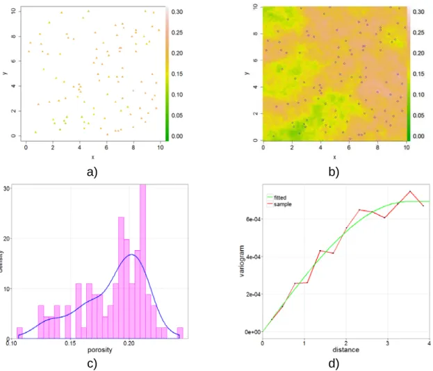
The data analysis procedures are schematically illustrated on Figure 1-1 for a synthetic data set which consists of 100 measurements of porosity on a territory of 10 × 10 𝑘𝑚2_{, see Figure 1-1(a). The histogram of the sample data is given at Figure}

1-1(c) and a smooth density model is fitted. The variogram analysis with a fitted spherical covariance model is demonstrated on Figure 1-1(d). Finally, a conditional simulation of a random field which respects the data at sample locations and the

(11)

9 fitted distribution is depicted of Figure 1-1(b). The blue circles indicate the sample locations.

a) b)

c) d)

Figure 1-1. Elements of geostatistical simulation workflow a) a set of 100 samples b) conditional simulation c) fitting a smooth density model d) fitting a smooth variogram

model variogram analysis

For the purpose of geostatistical simulation and prediction, it is often assumed that the investigated RF 𝑍(𝑥) with a covariance function 𝐶(𝑥, 𝑥′) is a transformation of a multivariate Gaussian RF 𝑌(𝑥) with a covariance function 𝜌(𝑥, 𝑥′): 𝑍(𝑥) = 𝜑(𝑌(𝑥)), where 𝜑(𝑧) is the normal score transform function (Chilès & Delfiner 2012). In that case it is common to perform data analysis for 𝜌(𝑥, 𝑥′) with the methods described above. This thesis uses extensively the hypothesis that 𝑍(𝑥) is a transform of a multivariate Gaussian RF 𝑌(𝑥) and hereafter we consider that 𝜌(𝑥, 𝑥′) was derived from the data analysis workflow.

1.5 Problem statement

We consider the problem of simulating a random field (RF) 𝑍(𝑥) with a marginal distribution 𝐹(𝑧) and a covariance function 𝐶(𝑥, 𝑥′) defined in the region 𝐷 ∈ 𝑅𝑑_,_{𝑑 = 1,2,3 on an unstructured grid. If the values of 𝑍(𝑥) are known at some}

(12)

10 points of 𝐷 (i.e. 𝑍(𝑑_𝑖) = 𝑧_𝑖, 𝑖 = 1 … 𝑁_{𝑑𝑎𝑡𝑎}), we say that the random field 𝑍(𝑥) is conditioned to data {(𝑑_𝑖, 𝑧_𝑖), 𝑖 = 1 … 𝑁_{𝑑𝑎𝑡𝑎}}. An unstructured grid can be defined as a finite number 𝑁_𝑏 of non-overlapping blocks {𝑣_𝑝, 𝑝 = 1 … 𝑁_𝑏} on 𝐷.

The goal of geostatistical simulation on unstructured grid is to simulate a random vector �𝑍�𝑣_𝑝� = _|𝑣1

𝑝|∫ 𝑍(𝑥)𝑑𝑥𝑣𝑝 , 𝑝 = 1 … 𝑁𝑏� of average values of 𝑍(𝑥) over the blocks of the grid which respects two conditions:

1) Correctly reproduces the marginal distribution – the marginal distribution of each component 𝑍(𝑣_𝑝) should coincide with the marginal distribution of

1

|𝑣𝑝|∫ 𝑍(𝑥)𝑑𝑥𝑣𝑝 . This property is referred to as volume support effect, since the distribution of 𝑍(𝑣_𝑝) is a function of the block 𝑣_𝑝.

2) The covariance between each pair of components 𝑍(𝑣_𝑝) and 𝑍(𝑣_𝑞) should coincide with the covariance between two stochastic integrals

1

|𝑣𝑝|∫ 𝑍(𝑥)𝑑𝑥𝑣𝑝 and

1

|𝑣𝑞|∫ 𝑍(𝑥)𝑑𝑥𝑣𝑞 .

The definition of the conditional simulation on unstructured grids is given only in the terms of first and second order statistics, which means that the distribution of the random vector �𝑍�𝑣_𝑝�, 𝑝 = 1 … 𝑁_𝑏� is not defined in a unique manner. One could also remark that this definition does not mention the conditioning data {(𝑑_𝑖, 𝑧_𝑖), 𝑖 = 1 … 𝑁𝑑𝑎𝑡𝑎}. In fact, the conditioning to data is included in this definition implicitly, since

the RF 𝑍(𝑥) respects the data 𝑧_𝑖 at locations 𝑑_𝑖,as stated in the beginning of the sections.

1.6 Related research

Simulations on unstructured grid can be performed by simulating on a fine scale regular grid followed by upscaling. Any type of simulation method on regular grids can be applied in this case, such as SGS, Cholesky decomposition, spectral simulation and others (Chilès & Delfiner 2012; Goovaerts 1997). This approach is detailed in Chapter 2.

Algorithms based on the direct sequential simulation (DSS) approach can be applied for simulations on unstructured grids. In this work we investigate two DSS algorithms: DSS-1 proposed by Soares (2001) and DSS-HR (direct sequential simulation with histogram reproduction) proposed by (Oz et al. 2003). Application of DSS-HR to the problem of simulations on unstructured grids was proposed by Manchuk et al. (2005). DSS algorithms are also discussed in Chapter 2.

This thesis proposes a theoretical framework for geostatistical simulations on unstructured grids based on the discrete Gaussian model (DGM). Previously DGM was applied to geostatistical simulations on regular grids (Emery 2009; Emery & Ortiz

(13)

11 2011), where DGM was used for conditional simulation and co-simulation. Another application of DGM for geostatistical simulations can be found in Brown et al. (2008), where the DGM is conditional simulation of Cox process on a regular grid with samples defined on various supports. The generalization of the DGM for unstructured grids in this thesis was derived independently of (Brown et al. 2008) and is deemed to be applied in a different context – on unstructured grids and with congruent samples defined on quasi-point support.

1.7 Thesis contributions

The main contributions of this thesis are:

1) Investigating the properties of DSS algorithms and providing simulation parameters for which DSS algorithms fail reproducing expected statistical properties.

2) Proposing two theoretical models (DGM 1 and DGM 2) based on DGM for geostatistical simulations of a continuous variable.

3) Investigating the theoretical difference between DGM 1 and DGM 2 and demonstrating this difference through a simulation test on a synthetic dataset.

4) Demonstrating that DGM-based simulation algorithms are not restricted to utilization of the sequential simulation paradigm and enable robust reproduction of marginal distribution and covariance.

5) Formalizing the problem of simulating discrete variables on unstructured grids and proposing a new theoretical model generalizing the pluri-Gaussian simulation model for facies on unstructured grids.

6) Investigating the problem of computing the block to block covariance on unstructured grids and demonstrating the advantage of Monte Carlo integration methods over other approaches. This research can be applied in a more general scope than geostatistical simulations, in particular, to the problem of prediction through block kriging.

(14)

12

Chapter 2: Geostatistical simulation methods for

unstructured grids

Résumé

Différentes méthodes existantes de simulation géostatistique sur les maillages non-structurés sont analysées. Les deux approches principales peuvent être appliquées – la simulation sur un maillage fin régulier suivi par l’upscaling et la simulation «directe» - sans la transformation à l’échelle Gaussienne. Les propriétés de ces méthodes et leurs inconvénients sont examinées.

This chapter summarizes various geostatistical methods that can be applied for simulations on unstructured grids. Two main classes of algorithms are considered – fine scale simulations followed by upscaling, and direct block simulations on unstructured grids. We refer to the fine scale simulation approach as “conventional”, since it requires little additional development relative to the geostatistical algorithms on regular grids. The direct block simulation algorithms do not use intermediate regular fine scale grids, and operate directly on the blocks of the target unstructured grid.

2.1 Conventional approach to simulations on unstructured grids

The straightforward approach for simulating on an unstructured grid is to use an auxiliary regular fine scale grid to perform a point support simulation on it and to upscale subsequently the results to the target unstructured grid. The classical inputs to a geostatistical simulation in petroleum industry are point data of a petrophysical property, the corresponding histogram and a covariance model. A number of simulation algorithms exist, whose implementation requires various additional theoretical assumptions.

The classical and the most commonly used assumption about the spatial structure of the random field to be simulated is the multivariate Gaussian assumption, which states that 𝑍(𝑥) is a (usually non-linear) transform of a multivariate Gaussian random field 𝑌(𝑥). Thus, 𝑍(𝑥) = 𝜑(𝑌(𝑥)), where 𝜑(𝑦) is the Gaussian anamorphosis function (Chilès & Delfiner 2012). The assumption of multigaussianity enables to simulate the Gaussian random field using numerous existing techniques like sequential Gaussian simulation (SGS), see Goovaerts (1997) for details and turning bands (Chilès & Delfiner 2012), among others. The above-mentioned methods provide simulations of a random field which is only approximately multivariate Gaussian due to assumptions used. A spectral simulation method for accurate generation multivariate Gaussian random fields on regular grids in 1D, 2D and 3D was proposed by Pardo-Iguzquiza and Chica-Olmo (1993). The final result of the simulation is obtained by transforming the simulated Gaussian field to the original scale using the anamorphosis 𝜑.

(15)

13 Another approach to the simulation of random fields given a histogram and a covariance is provided by a family of direct sequential simulation (DSS) algorithms. In that case no explicit assumption about the multivariate distribution of 𝑍(𝑥) is done, but a set of conditional distributions is explicitly provided. Different algorithms suggest using different local CDF in the sequential simulation procedure (Oz et al. 2003; Soares 2001). The ability of the direct sequential simulation approach to reproduce the target histogram and covariance was illustrated by Robertson et al. (2006). This approach has the advantage of avoiding the transformation to a Gaussian variable, although it raises problems concerning the internal consistency of the model used. For example, even though it is proven mathematically that a spherical covariance model is not compatible with a multivariate-lognormal random field (Matheron 1989), it is possible to perform a simulation using the DSS algorithm with such a construction. Obviously, in this case, the simulated random field will not correspond to the input parameters.

In the general case not every chain of local CDF defines a valid multivariate distribution function. Theoretical conditions for defining a valid multivariate distribution function from a set of conditional CDFs are provided by Cressie and Wikle (2011). In practice, it is not possible to verify these conditions; however, they form a valuable theoretical result.

After performing a simulation of the target random field 𝑍(𝑥) on a fine scale grid whose cells can be considered as point support, the results are upscaled on the target unstructured grid. The approach of using a fine scale grid for simulations has the advantage of avoiding assumptions about the change of support law for the random field 𝑍(𝑥) as well as assumptions about spatial distribution of the block average values 𝑍(𝑣). The fine scale simulations are especially efficient for simulating the variables that do not average linearly over the volume, such as permeability. In that case, the results of fine scale simulation can be upscaled on an unstructured grid using one of the numerical methods (Farmer 2002). The simulation algorithms which operate directly on blocks have to introduce additional assumptions and transform permeability to a variable that averages linearly.

From the practical point of view, using fine scale grids and upscaling on an unstructured grid does not always seem an optimal solution. This approach has a set of disadvantages such as creating and storing an auxiliary fine scale grid, increasing the number of locations at which the random field should be simulated and transferring the results from the fine regular to the unstructured grid – a process which can be time demanding and results in artifacts if the chosen refinement level was not sufficient for the given problem. When dealing with fine scale regular grids it remains a subjective decision which level of refinement should be chosen. It is clear that the size of the blocks in the fine scale regular grid should be at least as small as the smallest block in the target unstructured grid (otherwise there will not be any simulated values for the smallest block of the unstructured grid). This consideration

(16)

14 leads to necessity of using fine scale grids with several millions of blocks even if the target unstructured grid has a relatively small number of blocks, but high variability in the block sizes.

2.2 Direct sequential simulation on blocks

The goal of geostatistical simulation on block support is to avoid point support simulations and subsequent upscaling, and rather to simulate a random vector {𝑍(𝑣𝑖), 𝑖 = 1 … 𝑁}, where 𝑍(𝑣) denotes the average value of 𝑍(𝑥) over a grid block 𝑣.

The classical multigaussian formalism is not applicable on the block support, since the data do not average linearly after the normal score transform.

The family of DSS algorithms does not use the normal score transform and could be applied to simulations directly on the block support by merely replacing the kriging step of the SGS algorithm by a block kriging step. From the theoretical standpoint DSS is based on two mathematical methods: sequential simulation (Goovaerts 1997) and simple kriging principle (Journel 1993). The sequential simulation paradigm states that the simulation of a multivariate random vector can be done in a sequential manner. It is based on the well-known decomposition

P(A1,A2,…,AN) = P(A1)P(A2 | A1)P(AN | A1,…AN-1) where P is a probability measure

and (A1,A2,…AN) is any family of events (Shiryaev 1996). It can be applied whenever

all conditional distributions of a variable given all previously simulated variables are known. This decomposition is the basis for the classical SGS algorithm, in which the full conditional distribution is usually approximated by a conditional distribution using only the nearest previously simulated points. The simple kriging principle states that a sequential simulation procedure is able to reproduce the target covariance model as soon as the mean and variance of the conditional distribution at the iterations of the algorithm are determined by simple kriging. It is the simple kriging principle that enables correct reproduction of the covariance relations between blocks determined by the point-to-point covariance model 𝐶(ℎ). The possibility of applying two DSS algorithms DSS 1 (Soares 2001) and DSS-HR (Oz et al. 2003) for geostatistical simulations on unstructured grids is considered below. When the simulated variable 𝑍(𝑥) has a Gaussian marginal distribution DSS 1 and DSS-HR coincide with the classical SGS. Therefore one should examine the applicability of these algorithms for simulating distributions which depart from the Gaussian assumption, such as strongly skewed or heavy tailed distributions.

For testing purpose, consider a random field 𝑍(𝑥) following a lognormal distribution with logarithmic mean 0 and logarithmic variance 1. Its variance is thus 𝜎2 _{= 𝑒(𝑒 − 1). Since one of the key requirements to a geostatistical simulation}

algorithm on an unstructured grid is the correct reproduction of block to block covariance, it is necessary to verify that the simulation algorithm follows the simple

(17)

15 kriging principle, which ensures that the covariance is reproduced. In the case of a lognormal random field, the normal score transform 𝑦 = 𝜑−1(𝑧) = ln 𝑧 for 𝑍(𝑥) is known analytically. An analytical verification for DSS 1 is easily done within these settings. The algorithm DSS 1, as originally presented in Soares (2001), proceeds as follows:

1) Simple kriging is performed at location x, conditional on surrounding values, thus yielding a kriging prediction 𝑧∗(𝑥), and a kriging variance, 𝜎_𝑠𝑘2(𝑥).

2) The kriging prediction is then transformed to a normal score 𝑦∗(𝑥) = 𝑙𝑛 (𝑧∗_{(𝑥 )).}

3) A Gaussian random variable Y ∼ G � y∗(x),σsk2 (x)

σ2 � is drawn. 4) The simulated value at point 𝑧(𝑥) is then set equal to 𝑒𝑌.

Thus, 𝑍(𝑥) is lognormal with logarithmic mean 𝑙𝑛�𝑧∗(𝑥 )� and shape parameter

𝜎_𝑠𝑘2(𝑥)

𝜎2 . The mean and variance of the local CDF at location 𝑥 can be determined

𝐸𝑍(𝑥) = 𝑒𝑙𝑛�𝑧∗(𝑥 )�+𝜎𝑠𝑘 2 _(𝑥) 2𝜎2 _{= 𝑧}∗_{(𝑥 ) × 𝑒}𝜎𝑠𝑘 2 _(𝑥) 2𝜎2 _, (2.1) 𝑉𝑎𝑟 𝑍(𝑥) = �𝑒𝜎𝑠𝑘 2 _(𝑥) 𝜎2 _{− 1 � 𝑒}2𝑙𝑛�𝑧∗(𝑥 )�+𝜎𝑠𝑘 2_(𝑥) 𝜎2 = 𝑧∗_{(𝑥 )}2_{× 𝑒} 𝜎𝑠𝑘 2_(𝑥) 𝜎2 _�𝑒 𝜎𝑠𝑘 2_(𝑥) 𝜎2 _{− 1�.} (2.2) Obviously, both mean and variance (𝐸𝑍(𝑥), 𝑉𝑎𝑟 𝑍(𝑥)) are significantly different from the simple kriging mean and variance (𝑧∗(𝑥 ), 𝜎_𝑠𝑘2 (𝑥)), so the conditions of the simple kriging principle are not satisfied and the reproduction of the covariance is not guaranteed. Moreover, the variance is proportional to the squared kriging prediction at the given point, which is explained by the proportional effect inherent to a lognormal variable (Chilès & Delfiner 2012). Summarizing this results, the DSS 1 algorithm does not respect the simple kriging principle (Journel 1993) on which it is based.

In contrast to DSS 1, the simulation algorithm DSS-HR (Oz et al. 2003), respects by construction the simple kriging principle, which guarantees the block-to-block covariance reproduction. As in the case of DSS 1, DSS-HR assumes that the local CDFs of 𝑍(𝑥) depend only on the simple kriging mean and variance at a specific location. The algorithm consists in building a table of conditional CDF for 𝑍(𝑥) in a constructive manner presented in (Oz et al. 2003), indexing this family of distributions by their mean and variance and using the distribution with correct mean and variance at every step of the sequential simulation. By construction, the indexed table of local distributions of 𝑍(𝑥) is congruent with a table of Gaussian distributions.

(18)

16 When transferring the data from point to block support, it is expected that the mean value of the block is determined by the mean value of the point-support random field and the variance is determined by the point-support covariance and the block geometry (in the absence of conditioning data). DSS-HR is proven to preserve the mean of the simulated property and to reproduce the correct block-to-block covariance, despite the fact that the constructive manner of generating the set of conditional CDFs has certain theoretical drawbacks. DSS-HR implies marginal distributions for grid blocks which are not necessarily compatible with a random field distributed on point support. Thus, for any spatial random field 𝑍(𝑥) with a covariance function 𝐶(𝑥, 𝑥′) and with a finite integral range 𝐴 = ∫ 𝐶(𝑥, 𝑥′)_𝑅₃ 𝑑𝑥𝑑𝑥′ due to the central limit theorem (CLT) the distribution of the average 𝑍(𝑣) of the block 𝑣 tends to a Gaussian distribution with mean equal to the global mean, and variance

1

|𝑣|2∫ ∫ 𝐶(𝑥, 𝑥_𝑣 _𝑣 ′)𝑑𝑥𝑑𝑥′ which decreases as the block size becomes larger. This property of the average value is often expected by the practitioners; the general proof of this statement goes beyond the scope of the present work. The compatibility with the CLT for DSS-HR does not follow straightforward from the simulation algorithm. In order to test the compatibility of DSS-HR with the CLT, one should investigate the dependence of the marginal distribution of a block depending on the size of this block. Algorithm DSS-HR implicitly assumes by construction that the unconditional marginal distribution of every block is contained in the pre-computed CDF table along with conditional distributions. It is also assumed that this marginal distribution is determined solely by the global mean and the variance of the block and this fact is used in the first step of the sequential simulation procedure.

When performing multiple unconditional simulations of a reservoir model with a given CDF table, one can expect that the marginal distribution of a given block coincides with the distribution from the CDF table which corresponds to the global mean and unconditional variance of that block only if the table of conditional distributions defines a valid multivariate distribution function. For the test it is assumed that the corresponding distribution from the table is observed. In practice, the observed distribution depends on implementation details, particularly regarding the neighborhood used for the computation of the kriging predictor and the kriging variance. The marginal distribution predicted by DSS-HR for a given block is now investigated. It should be noted that, when simulating a single block, the conditional CDF table always defines a valid multivariate distribution function. In this particular case, the assumption above is valid.

Consider a simulation of a RV with a point-support marginal distribution defined by a CDF at Figure 2-1(a). This function is selected for the test, since it has a marked difference in behavior in the neighborhood of (6, 0.25), the abscissa of which corresponds to the mean of the RV defined by this CDF. The mean and variance of the CDF at Figure 2-1 (a) are equal to 6 and 4 respectively. The distribution under concern enables to illustrate how the properties of the input CDF

(19)

17 are preserved by DSS-HR for all the generated distributions. It should be noted that the covariance model is not important for this test, since the block marginal distributions provided by DSS-HR and DGM can be parameterized if the block mean and variance are known. Figure 2-1(b) illustrates the CDF for a block with the variance 0.4 implied by DSS-HR for the point-support distribution from Figure 2-1(a) compared to CDF implied by DGM and to the normal distribution.

(a) (b)

Figure 2-1. Marginal distributions for (a) point support and (b) selected block support for DSS-HR, DGM 2 (see Chapter 3) and Gaussian distribution.

Figure 2-1(b) shows that even for a variance reduction factor 10 (ratio of the point-support variance to the block-support variance) the block marginal distribution proposed by DSS-HR preserves the shape of the input distribution in the neighborhood of (6, 0.25) and does not converge to the normal distribution. This behavior can be explained by the constructive manner of generating the table of CDFs. This effect is less noticeable for smooth CDF functions.

DGM 2 DSS-HR Normal

(20)

18

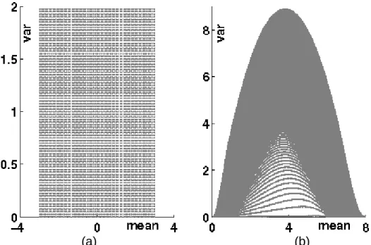
(a) (b)

Figure 2-2. Scatter plot of pairs (mean, variance) for (a) Gaussian distributions and (b) corresponding local distributions generated by DSS-HR algorithm

A table of conditional distributions was generated for this test according to the DSS-HR algorithm. Figure 2-2 illustrates the link between the space of the Gaussian distributions and the space of the distributions constructed for the test. The example provided on Figure 2-1(a-b) shows that the applicability of DSS-HR should be tested in every particular problem and that it is unlikely that the proposed constructive algorithm could be used as a change of support model in the general case, especially for random fields with a non smooth CDF. In addition to this, DSS-HR is limited by the sequential simulation principle and suffers from the weakness of all the sequential simulation algorithms – necessity of using a limited neighborhood in the simulation. As it is demonstrated in Chapter 3, using local neighborhoods in the sequential simulation leads to underestimation of the theoretical covariance between the blocks.

(21)

19

Chapter 3: Discrete Gaussian model for

Unstructured Grids

Résumé

Une nouvelle méthode de simulation sur les maillages non-structurés est présentée – la simulation avec le modèle Gaussien discret. Deux versions théoriques de ce modèle sont décrites – DGM 1 et DGM 2, la différence entre ces deux versions étant démontrée de façon analytique et avec un exemple synthétique de gisement. Une solution au problème de conditionnement des simulations est proposée, les aspects avancés des simulations géostatistiques sont discutés – à savoir le traitement des variables non-additives et des variables co-régionalisées.

3.1 Introduction

The Discrete Gaussian Model was originally proposed by Matheron (1976a) as a solution for approximate computation of transfer functions (conditional laws of blocks within a panel). The problem considered by Matheron (1976a) was of practical importance for the mining industry – each block within a panel is dispatched either to waste or to the mill. In order to predict the future production, It is important to assess the number and the average grade of the blocks within a panel whose grade is higher than the selected cut-off grade value. Emery (2007) investigates the properties of the DGM along with other change of support models (Hermitian, Laguerrian) and provides a simplified method for deriving the change of support coefficient and covariance between the transformed variables.

The application of DGM to geostatistical simulations is due to (Emery 2009; Emery & Ortiz 2011). In their papers authors apply DGM in the form stated in (Emery 2007) to the problem of geostatistical simulations on regular grids. As demonstrated by authors, DGM enables reducing the problem of geostatistical simulation of a continuous parameter on a regular grid with change of support effect to a problem of simulating a multivariate Gaussian random field and applying appropriate transformation functions. The main difference in application of DGM in (Emery 2009) and (Emery & Ortiz 2011) consists in using either turning bands or spectral simulation for generating the multivariate Gaussian random vectors. In this thesis we separate the theoretical model for geostatistical simulations on unstructured grids from the implementation of the simulation algorithm. The theoretical models developed in this thesis rely on the multivariate Gaussian random fields and thus the simulation algorithm requires simulating realizations of multivariate Gaussian random vectors. As it is demonstrated further in this chapter, various methods can be used as subroutines for simulating multivariate Gaussian random vectors which leads to different accuracy for the reproduction of the desired statistics.

(22)

20 A generalization of DGM for samples of different sizes was given in Brown et al. (2008), which presents a theoretical framework for incorporating multiple scale samples data on a regular grid. In Brown et al. (2008), an approach based on graphical models representation for grid blocks and samples and on the DGM variant from Emery (2007) is proposed. An extended version of the conditional independence assumption is then used to derive the covariance matrix between the block-transformed variables. This approach is deemed to be applicable in the mining industry, whereas this thesis proposes an approach for incorporating point-support distribution and spatial variation information on geological models with varying block size which is a common problem in petroleum reservoir engineering.

This thesis presents a generalization for unstructured grids of the classical DGM in the form given in (Chilès & Delfiner 2012). The random field 𝑍(𝑥) = 𝜑(𝑌(𝑥)) with covariance function 𝐶(𝑥, 𝑥′) is considered to be an anamorphosis (i.e., a strictly monotonic transform) of a Gaussian random field 𝑌(𝑥) with covariance function 𝜌(𝑥, 𝑥′). Let {𝜑𝑖, 𝑖 = 0 … ∞} denote the coefficients of decomposition of 𝜑(𝑦) in the

basis of normalized Hermite polynomials {𝜒_𝑖(𝑦), 𝑖 = 0 … ∞} 𝜑(𝑦) = � 𝜑𝑖𝜒𝑖(𝑦)

∞

𝑖=0 , (3.1)

The covariance functions 𝐶(𝑥, 𝑥′) and 𝜌(𝑥, 𝑥′) are related through Eqn.(3.2), see (Chilès & Delfiner 2012)

𝐶(𝑥, 𝑥′) = � 𝜑𝑖2𝜌(𝑥, 𝑥′)𝑖 ∞

𝑖=1

(3.2)

A subscript 𝑥 will further denote a uniformly distributed randomized location of a point in the block 𝑣 containing this point. For 𝑥 belonging to a specific block 𝑣_𝑝, the random variable 𝑌(𝑥) is denoted 𝑌_𝑝.

The key assumption of the generalized DGM is that the average values of the blocks �𝑍�𝑣_𝑝�, 𝑝 = 1 … 𝑁_𝑏� are block-dependent transforms of random variables with standard Gaussian distribution

𝑍�𝑣𝑝� = 𝜑𝑣𝑝(𝑌𝑣𝑝), 𝑝 = 1 … 𝑁. (3.3) A positive real number 𝑟_𝑝 called the block change of support coefficient is associated with each block 𝑣_𝑝. By definition 𝑟_𝑝 is the correlation coefficient between 𝑌𝑣𝑝 and 𝑌𝑝

𝑟𝑝 = 𝑐𝑜𝑣(𝑌𝑣𝑝, 𝑌𝑝). (3.4)

The success of applying the DGM to the problem of geostatistical simulations on unstructured grids is due to the high quality of reproduction of the true marginal

(23)

21 distributions of the block values 𝑍(𝑣) = 1

|𝑣|∫ 𝑍(𝑥)𝑑𝑥𝑣 . As demonstrated analytically by

Matheron (1985), DGM provides a second order accurate approximation of the density of the average value 𝑍(𝑣) in the case of a multigaussian diffusion-type random fields, when the support 𝑣 is constant throughout the domain.

The advantage of DGM relative to DSS algorithms is the compatibility with the central limit theorem (CLT). Indeed, when the change of support coefficient 𝑟_𝑣 for a block 𝑣 is small, the block transformation function 𝜑_𝑣(𝑦) can be written in the following form (Chilès & Delfiner 2012)

𝜑𝑣(𝑦) = 𝜑0+ 𝜑1𝑟𝑣𝑦 + ∆(𝑟𝑣), (3.5)

where ∆(𝑟_𝑣) is small relative to 𝑟_𝑣. And thus for small values of 𝑟_𝑣

𝑍(𝑣) ≈ 𝜑0+ 𝜑1𝑟𝑣𝑌𝑣. (3.6)

We start presentation of two generalizations (DGM 1 and DGM 2) of DGM from considering unconditional simulations. The additional assumptions required for conditioning will be considered after.

(24)

22

3.2 Discrete Gaussian model 1

In order to derive the theoretical model for the unconditional simulation �𝑍�𝑣𝑝�, 𝑝 = 1 … 𝑁𝑏� of a random field 𝑍(𝑥) with marginal distribution 𝐹(𝑧) and

covariance function 𝐶(𝑥, 𝑥′) on an unstructured grid �𝑣_𝑝, 𝑝 = 1 … 𝑁_𝑏�, assumption about existence of underlying Gaussian random vector �𝑌_𝑣_𝑝, 𝑝 = 1 … 𝑁_𝑏� is done as on Eqn. (3.3). The first generalized Discrete Gaussian Model (DGM 1) requires two main hypotheses, which are sufficient to produce unconditional simulations on unstructured grids that respect marginal and bivariate distributions:

i. The vector (𝑌_𝑣₁, … 𝑌_𝑣

𝑁𝑏) is stationary multivariate Gaussian;

ii. For every block 𝑣_𝑝 the joint distribution of 𝑌_𝑣_𝑝 and the value at the random point within the block 𝑌_𝑝 is bivariate Gaussian with correlation coefficient 𝑟_𝑝. It is shown below, that the above assumptions are sufficient to convert the initial problem to a problem of generating unconditional Gaussian fields and deriving all the unknown parameters. Using Cartier’s relation (Chilès & Delfiner 2012) p. 441

𝐸�𝑍�𝑥��𝑍(𝑣)] = 𝑍(𝑣) (3.7)

assumption (ii) enables the derivation of the block-specific transform functions 𝜑_𝑣_𝑝(𝑦) for every block 𝑣_𝑝

𝜑𝑣𝑝(𝑦) = � 𝜑𝑖𝑟𝑣𝑖𝑝𝜒𝑖(𝑦)

∞

𝑖=0 , (3.8)

where {𝜒_𝑖(𝑦), 𝑖 = 0 … ∞} is the basis of normalized Hermite polynomials. This decomposition of 𝜑_𝑣_𝑝(𝑦) in the Hilbertian basis allows deriving the change of support coefficients for blocks. Indeed, since {𝜒_𝑖(𝑦), 𝑖 = 0 … ∞} are orthogonal with respect to the scalar product induced by the density of the normal distribution 𝑔(𝑦), one can derive it using the point-support covariance 𝐶(𝑥, 𝑥′) of 𝑍(𝑥) and properties of isofactorial models (Chilès & Delfiner 2012; Rivoirard 1994)

𝑉𝑎𝑟 �𝑍𝑣𝑝� = 1 |𝑣|2� � 𝐶(𝑥, 𝑥′)𝑑𝑥𝑑𝑥′= � 𝜑𝑖2𝑟𝑝2𝑖 ∞ 𝑖=0 𝑣 𝑣 , (3.9)

which leads to a polynomial equation on 𝑟_𝑝.

Assumption (i) permits to derive the covariance matrix for the random vector (𝑌𝑣1, … 𝑌𝑣𝑁). Indeed, the covariance 𝑅𝑝𝑞 between any two variables 𝑌𝑣𝑝 and 𝑌𝑣𝑞 can be determined through the following identity in the same manner as in Eqn. (3.9)

𝑐𝑜𝑣 �𝑍𝑣𝑝, 𝑍𝑣𝑞� = 1 |𝑣𝑝||𝑣𝑞| � � 𝐶(𝑥, 𝑥 ′_{)𝑑𝑥𝑑𝑥}′ 𝑣𝑞 𝑣𝑝 = � 𝜑𝑖2𝑟𝑝𝑖𝑟𝑞𝑖𝑅𝑝𝑞𝑖 ∞ 𝑖=1 . (3.10)

(25)

23 The equations above enable the determination of the change of support coefficients �𝑟_𝑝, 𝑝 = 1 … 𝑁_𝑏� and of the correlation coefficients �𝑅_𝑝𝑞, 𝑝 = 1 … 𝑁_𝑏, 𝑞 = 1 … 𝑁𝑏}. This converts the problem of generating a non-stationary random vector

{𝑍(𝑣𝑖), 𝑖 = 1 … 𝑁𝑏} to a classical problem of generating a multivariate Gaussian

random vector {𝑌_𝑣_𝑝, 𝑝 = 1. . 𝑁_𝑏} with a given covariance matrix which can be solved by classical methods for simulating multivariate Gaussian random vectors (e.g. SGS). Application of block-specific transformation functions 𝜑_𝑣_𝑝(𝑦) provides a realization of {𝑍�𝑣𝑝�, 𝑝 = 1 … 𝑁𝑏}.

The accuracy of reproduction of the correct marginal distribution was demonstrated analytically for small change of support (Matheron 1985). For practical applications, results of numerous Monte Carlo simulations are available (Chilès 2014; Chilès & Delfiner 2012). The advantage of DGM 1 is the correct reproduction of the covariance between different blocks. Indeed, using the block-specific transformation functions and covariance between the components of the Gaussian vector derived above leads to the theoretically correct block to block covariance defined by the covariance function 𝐶(𝑥, 𝑥′) 𝑐𝑜𝑣 �𝑍𝑣𝑝, 𝑍𝑣𝑞� = 1 |𝑣𝑝||𝑣𝑞| � � 𝐶(𝑥, 𝑥 ′_{)𝑑𝑥𝑑𝑥}′ 𝑣𝑞 𝑣𝑝 , (3.11)

(26)

24

3.3 Discrete Gaussian model 2

This model is a generalization of another version of the DGM presented in (Emery 2007; Rivoirard 1994). At the cost of a third, more restrictive, assumption which will be detailed below, it provides a simpler approach for computing the change of support coefficients and covariance relations as compared to DGM 1. Since adding a more restrictive assumption implies that the model is less likely to fit the data, the price to pay is in some cases less accuracy in reproducing the histogram of the simulated property (Chilès 2014; Chilès & Delfiner 2012). There are also some theoretical consistency drawbacks that will be discussed. The additional assumption characterizing DGM 2 is:

iii. for any block 𝑣 and two independent randomized locations 𝑥 and 𝑥′ within 𝑣, the joint distribution of 𝑌(𝑥) and 𝑌(𝑥′) is bivariate Gaussian.

One can derive from assumption (iii) the following relation for 𝑌_𝑣 and 𝑌(𝑣) =

1

|𝑣|∫ 𝑌(𝑥)𝑑𝑥𝑣 for every block (Chilès & Delfiner 2012; Emery 2007)

𝑌(𝑣) = 𝑟𝑣𝑌𝑣, (3.12)

which provides a simple formula for computing the change-of-support coefficient 𝑟_𝑣 for every block 𝑣 (Emery 2007)

𝑉𝑎𝑟�𝑌(𝑣)� = _{|𝑣||𝑣| � �𝜌}1 (𝑥, 𝑥′_{)𝑑𝑥𝑑𝑥}′ 𝑣

𝑣 = 𝑟𝑣

2_. _(3.13)

In an analogous manner, for any blocks 𝑣_𝑝 and 𝑣_𝑞, the covariance 𝑅_𝑝𝑞 between 𝑌_𝑣_𝑝 and 𝑌_𝑣_𝑞 is 𝑅𝑝𝑞 = _𝑟1 𝑝𝑟𝑞𝑐𝑜𝑣 �𝑌�𝑣𝑝�, 𝑌�𝑣𝑞�� = 1 𝑟𝑝𝑟𝑞 1 �𝑣𝑝��𝑣𝑞�� 𝜌(𝑥, 𝑥′)𝑑𝑥𝑑𝑥 ′ 𝑣𝑞 𝑣𝑝 . (3.14)

Using covariance matrix {𝑅_𝑝𝑞, 𝑝 = 1 … 𝑁_𝑏, 𝑞 = 1 … 𝑁_𝑏} an unconditional realization of vector (𝑌_𝑣₁, … 𝑌_𝑣

𝑁𝑏) can be generated.

The theoretical cost of the additional assumption of DGM 2 is relatively high. It is not obvious, whether there exists a random field 𝑌(𝑥) for which the joint distribution of the values at two random locations �𝑌�𝑥�, 𝑌�𝑥′�� is bivariate Gaussian. Even in the case of a multivariate Gaussian 𝑌(𝑥), the joint distribution of the vector �𝑌�𝑥�, 𝑌�𝑥′_{�� is a mixture of bivariate Gaussian distributions with different correlation}

coefficients, which is known to be non-Gaussian, but Hermitian bivariate distribution. Indeed, suppose 𝑥 and 𝑥′ belong to the same block 𝑣. Due to the uniform distribution and to the independence of the randomized locations, it follows

(27)

25 𝑃�𝑌�𝑥� ≤ 𝑦1, 𝑌�𝑥′� ≤ 𝑦2� =_|𝑣|1₂� �𝑃(𝑌(𝑥) ≤ 𝑦1, 𝑌(𝑥′) ≤ 𝑦2)𝑑𝑥𝑑𝑥′ 𝑣 𝑣 = ∫ 𝐺𝜌(𝑦1, 𝑦2)𝜔(𝑑𝜌), (3.15)

where 𝐺_𝜌denotes the bivariate standard Gaussian distribution with correlation coefficient 𝜌 and 𝜔(𝑑𝜌) denotes the density of 𝜌. This formula proves that the joint distribution of �𝑌�𝑥�, 𝑌�𝑥′�� is a mixture of standard Gaussian distributions with different correlation coefficients, which, according to (Matheron 1976b) is a Hermitian law with coefficients �𝑇_𝑖 = ∫ 𝜌𝑖𝜔 �𝑑𝜌� , 𝑖 = 0 … + ∞ �. In DGM 2 these coefficients are approximated as �𝑇_𝑖 ≈ 𝑟_𝑣2𝑖, 𝑖 = 0 … + ∞� with the block change of support coefficient 𝑟𝑣.

Moreover, for every block 𝑣 DGM 2 provides two different methods for computing the change of support coefficient 𝑟_𝑣, using Eq. (3.9) and Eq. (3.13), which in general provide different results (Chilès 2014). Whether the simpler approach for determining the model parameters of DGM 2 leads to a correct reproduction of the correlation between blocks was theoretically investigated. The following result was obtained.

Proposition 1

The covariance between the block average values 𝑍(𝑣_𝑝) and 𝑍�𝑣_𝑞� computed with DGM 2 is biased relative to the theoretical covariance 1

|𝑣𝑝||𝑣𝑞|∫ ∫ 𝐶(𝑥, 𝑥

′_{)𝑑𝑥𝑑𝑥}′ 𝑣𝑞

𝑣𝑝 between blocks 𝑣_𝑝 and 𝑣_𝑞.

The proof of this proposition is provided in Appendix A. The bias is introduced due to the additional theoretical assumptions of DGM 2. In Emery (2009), the author presents an algorithm for geostatistical simulations on regular grids using DGM 2. The result provided in Appendix A evaluates the bias in covariance implied by this algorithm in the particular case of two identical blocks on a regular grid. The above-mentioned bias is illustrated in the following section. However, in the practical applications of petroleum industry, the range of the covariance function is usually significantly larger than the grid block size along different dimensions (in the area of main interest at least). Hence, the accuracy of DGM 2 can be considered as sufficient.

(28)

26

3.4 Model testing

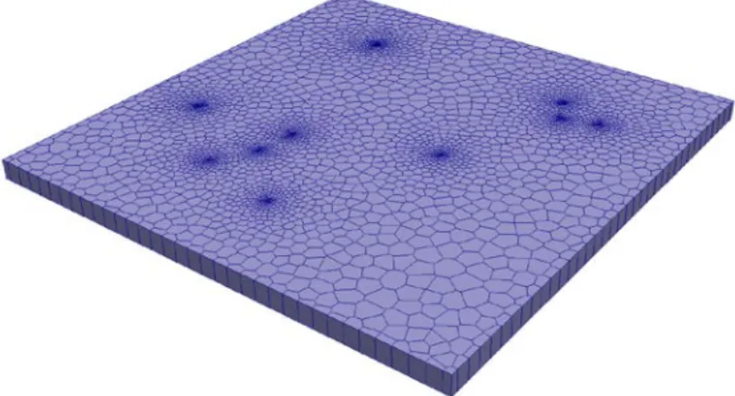
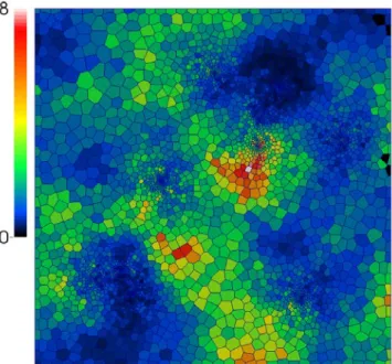
In order to demonstrate the application of DGM 1 and DGM 2 to geostatistical simulations on unstructured grids, a two-dimensional Voronoï polygon grid of 20x20 km2 is studied. The grid consists of 3,546 Voronoï polygon cells and includes 10 local grid refinement regions (LGR) in the areas of potential wells placement locations, the bounding box size for the smallest and the biggest blocks sizes are 36x42 and 1,035x1,052 m respectively. Figure 3-1 illustrates the studied grid highlighting the volumetric differences between the blocks.

Figure 3-1. The volume distribution of the studied grid. 4 blocks near the right border were excluded from computations; their volume is set to 0. White points indicate the

wells locations.

A simulation of a lognormal variable 𝑍(𝑥) = 𝜑(𝑌(𝑥)) with logarithmic parameters (0, 1) on the block support is considered using DGM 1, DGM 2 as well as conventional simulation on a fine regular grid with upscaling approaches. The covariance 𝜌(ℎ�) of the normal score transform variable 𝑌(𝑥) is considered to be known. For this test the isotropic spherical covariance with a small range of 250 m was used in order to test the accuracy of DGM 1 and DGM 2 for a variety of ratios between covariance range and block size. The covariance 𝐶(ℎ�) of 𝑍(𝑥) is computed numerically through formula (3.2).

Realization both of a conventional simulation and of a simulation with a DGM are illustrated on Figure 3-2(a-b). SGS was used for simulating the multivariate Gaussian random vectors. The results for DGM 1 and DGM 2 are visually similar, only the result for DGM 2 is provided. Based on 50,000 unconditional simulations, the observed distributions of the block values as well as the descriptive statistics of the simulated values were analyzed. The results obtained demonstrate satisfactory accuracy in approximating the real distribution of the average block values with DGM

(29)

27 1 and DGM 2 predicted densities. For small blocks the densities provided by DGM 1 and DGM 2 are undistinguishable on the plot. For the largest block in the model the comparison is given on Figure 3-3.

a)

b)

Figure 3-2. Simulation of a lognormal variable on a Voronoï polygon grid for spherical 𝜌(ℎ) with range 250m. a) using fine scale regular grid and upscaling. b) using DGM 2

(30)

28 Figure 3-3. Observed density for the value of the largest block in the grid, compared

to theoretical predictions of DGM 1 and DGM 2, based on 50,000 simulations Investigating the descriptive statistics of the block values enables to highlight the practical difference between application of DGM 1 and DGM 2. The variance of every block in the model was estimated from the sample and compared to the theoretical value of the block variance. Figure 3-4 demonstrates the mismatch �𝐶(𝑣, 𝑣) − 𝐶̂(𝑣, 𝑣)� of the estimated variance from the theoretical variance depending on the block volume.

As can be seen on Figure 3-4, the difference between the estimated and theoretical variance for the realizations produced by DGM 1 approach oscillates around 0, whereas DGM 2 approach demonstrates a bias in the variance which is derived analytically in Appendix A. It should be noted that the relative value of the bias does not exceed 5% of the a priori variance of 𝑍(𝑥). When the covariance range exceeds significantly the block dimensions, which is often encountered in practical applications, the difference between DGM 1 and DGM 2 can be neglected. A realization of the previous test with a covariance function range of 8 km is given on Figure 3-5(a-b).

(31)

29 Figure 3-4. Mismatch of the estimated variance from the theoretical variance of the

block defined by 𝐶(ℎ�) a)

(32)

30 b)

Figure 3-5. Simulation with a spherical covariance 𝜌(ℎ) with range 8 km using a) fine scale regular grid and upscaling b) DGM 2

Let us consider a more rigorous test for unconditional simulations on unstructured grids with DGM. Let us consider that the grid on Figure 3-1 is a 3D grid with the thickness of 40 meters (in order to introduce complexity into covariance computations), see Figure 3-6.

Figure 3-6. 3D grid with 10 local refinement zones. Vertical zoom factor 20. The reproduction of all block to block theoretical covariances 𝐶�𝑣_𝑝, 𝑣_𝑞� can be tested. We use 3 different input covariance models 𝜌�ℎ�� in 3D for the Gaussian variable 𝑌(𝑥) which is a normal score transform of 𝑍(𝑥):

1) Short range 𝜌₁(ℎ�) - spherical covariance with ranges (250m, 250m, 10m);

(33)

31 2) Long range 𝜌₂(ℎ�) - spherical covariance with ranges (5km, 5km, 0.2km); 3) Double structure 𝜌₃(ℎ�) – 0.75 Sph (250m, 250m, 10m) + 0.25 Sph(5km,

5km, 0.2km).

Case 3 represents a mixture of cases 1 and 2. The normalized to unit covariance functions 𝜌₁(ℎ) and 𝜌₃(ℎ) as well as the corresponding 𝐶₁(ℎ) and 𝐶₃(ℎ) are depicted on Figure 3-7.

Figure 3-7. Normalized covariance functions 𝜌₁(ℎ�), 𝜌₃(ℎ�) (left axis) and 𝐶₁(ℎ),𝐶₃(ℎ) (right axis) used for the test..

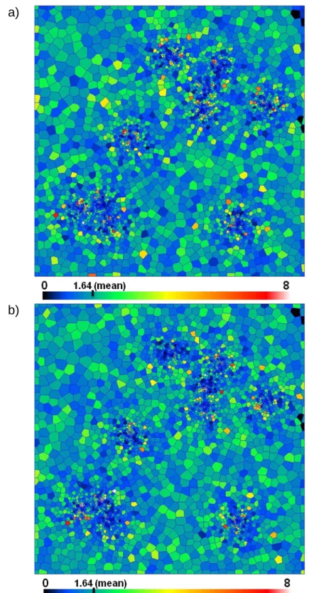
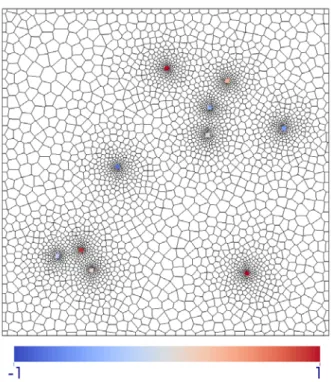
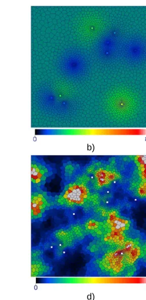
For each input covariance 𝜌_𝑖�ℎ��, 𝑖 = 1,2,3 of 𝑌(𝑥), the corresponding covariance 𝐶_𝑖(ℎ) of 𝑍(𝑥) is computed. Given 𝐶_𝑖(ℎ) the full matrix of the block to block covariance 𝐶�𝑣_𝑝, 𝑣_𝑞�, 𝑝 = 1 … 𝑁_𝑏, 𝑞 = 1 … 𝑁_𝑏 is computed and stored (since the matrix is symmetric and sparse, only pertinent values are stored). Multiple simulations are produced with DGM 1 and the covariance between each pair of blocks is estimated. The Gaussian random vector �𝑌_𝑝, 𝑝 = 1 … 𝑁_𝑏� is produced with SGS, taking 50 closest neighbors for the small range covariance 𝐶₁(𝑥, 𝑥′) and 200 neighbors for the other two cases. For case 1 – small range covariance 50000 simulations were produced, for cases 2 and 3, due to use of a significantly larger simulation neighborhood the number of produced realizations was reduced to 20000. Three different realizations produced with DGM 1 for small range, long range and double structure input covariance model are demonstrated on Figure 3-8.

The expected spatial behavior of the model is visually reproduced on Figure 3-8(a-c). Figure 3-8a,c demonstrate more spatial variation in refinement zones and less variation in the zones of large blocks. Spatial features of the expected size (5 × 5

(34)

32 km) are visible on Figure 3-8b,c. Figure 3-8c reproduces both the fine scale variations in the refinement zones and the large scale heterogeneities.

a) b)

c)

Figure 3-8. Simulations on an unstructured 3D grid for a) covariance with small range 𝐶1(ℎ) b) covariance with long range 𝐶2(ℎ) and c) double structure covariance 𝐶3(ℎ)

The scatter plots of the estimated covariance values versus the theoretical are demonstrated on Figure 3-9a-c (zero theoretical covariances are ignored). It is visible that the DGM 1 – based simulation method reproduces the block to block covariance for all 3 types of input covariance functions. For the purpose of this test, all block to block covariances were computed through approximating each block of the cell with 50 Sobol’ quasi-random points (see Chapter 5). Figure 3-9b,c shows that the dispersion covariance of the estimates increases with the increase of the theoretical covariance value. This behavior is in line with the theoretical model used – the most correlated blocks on the grid are the smallest ones, for which the simulated values are more dispersed.

The different neighborhood sizes (20 for small range and 200 for other cases) for this test were chosen by a trial method. It was observed that for a small range

(35)

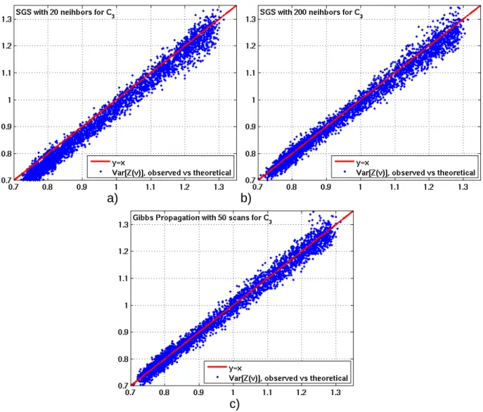
33 covariance 𝐶₁(ℎ�) using 20 neighbors is sufficient in order to reproduce block to block covariances, whereas significantly larger neighborhood is required for the long range covariance functions. Figure 3-10 illustrates the scatter plot of the observed block variances versus theoretical block variances for 𝐶₃(ℎ�). The results are obtained from 20,000 unconditional simulations. Figure 3-10a shows that when 20 neighbors are used for the double structure covariance, the block variance is systematically underestimated. Since by construction of the theoretical model DGM 1 respects the block to block covariance, the source of underestimation is the SGS procedure which was used to simulate multivariate Gaussian random vectors. This underestimation can be corrected with increasing the neighborhood size; indeed, Figure 3-10b shows that when 200 neighbors are used the underestimation diminishes. However, it remains noticeable, especially for large values of block variance.

a) b)

c)

Figure 3-9. DGM 1. Scatter plots of observed covariance versus theoretical covariance for a) covariance with small range 𝐶₁(ℎ�)b) covariance with long range

𝐶2(ℎ�) and c) double structure covariance 𝐶3(ℎ�)

This problem arises due to the fact that only a limited number of neighbors were used in SGS. Although the number of neighbors used (200) is relatively large for this type of problems (it is common to use less than 50 neighbors in practical

(36)

34 applications of petroleum industry, and sometimes only the cells which share a common side are used as neighbors), a systematic deviation from the theoretical values can be observed. The destructive effect for the model statistics due to the limited SGS neighborhood was noted in Emery (2004b) for the case of spherical variogram in 2D. As demonstrated in the same paper, increasing the neighborhood size improves the quality of the simulation. Except for special cases, such as simulating with exponential covariance function (Chilès & Delfiner 2012), there does not exist a theoretical relationship between the size of the neighborhood which should be used in SGS and the type of the simulated covariance model. The impact of the limited simulation neighborhood can be assessed as proposed by Emery and Peláez (2011).

a) b)

c)

Figure 3-10. Scatter plots of sample variance versus theoretical for 𝐶₃(ℎ�) for a) SGS with 20 neighbors b) SGS with 200 neighbors c) Gibbs Propagation algorithm with 50

scans.

This deviation from the theoretical values of block variance can be eliminated if a more reliable method for generating Gaussian random vector �𝑌_𝑝, 𝑝 = 1 … 𝑁_𝑏� is used. One of the alternatives of the SGS for simulating multivariate Gaussian random