Fatigue models for life prediction of structures under multiaxial loading with variation in time and space.

(1)

HAL Id: tel-01712901

https://pastel.archives-ouvertes.fr/tel-01712901

Submitted on 19 Feb 2018

HAL is a multi-disciplinary open access archive for the deposit and dissemination of sci-entific research documents, whether they are pub-lished or not. The documents may come from teaching and research institutions in France or abroad, or from public or private research centers.

L’archive ouverte pluridisciplinaire HAL, est destinée au dépôt et à la diffusion de documents scientifiques de niveau recherche, publiés ou non, émanant des établissements d’enseignement et de recherche français ou étrangers, des laboratoires publics ou privés.

Fatigue models for life prediction of structures under

multiaxial loading with variation in time and space.

Zepeng Ma

To cite this version:

Zepeng Ma. Fatigue models for life prediction of structures under multiaxial loading with variation in time and space.. Mechanics of the solides [physics.class-ph]. Université Paris-Saclay, 2017. English. �NNT : 2017SACLX117�. �tel-01712901�

(2)

NNT : 2017SACLX117

THÈSE DE DOCTORAT

DE

L’UNIVERSITÉ PARIS-SACLAY

PRÉPARÉE À

L’ÉCOLE POLYTECHNIQUE

ÉCOLE DOCTORALE N

◦

₅₇₉

Sciences mécaniques et énergétiques, matériaux et géosciences

Spécialité de doctorat : Mécanique des solides

Par

Monsieur Zepeng MA

A New Strategy for Fatigue Analysis in Presence of

General Multiaxial Time Varying Loadings

Thèse présentée et soutenue à Palaiseau, le 18 decembre 2017 Composition du Jury :

M. Georges CAILLETAUD Professeur, Mines ParisTech Président du Jury M. Franck MOREL Professeur, LAMPA ENSAM, Angers Rapporteur M. Nicolas SAINTIER Professeur, Arts et Métiers ParisTech Rapporteur M. Eric CHARKALUK Professeur, École Polytechnique Examinateur Mme Ida RAOULT Ingénieur de recherche, PSA Examinatrice M. Patrick LE TALLEC Professeur, École Polytechnique Directeur de thèse M. Habibou MAITOURNAM Professeur, ENSTA Paristech Co-encadrant

(3)

(4)

“The whole of science is nothing more than a refinement of everyday thinking.”

(5)

(6)

Acknowledgements

My thanks go to Prof. P. Le Tallec, dear supervisor of the thesis. I thank him for having assured the scientiﬁc quality in this work and for having also entrusted to me the responsibilities of my scientiﬁc productions. I will not repeat what was said on the day of the defense, but thanks to him I discovered France and polytechnique, a landscape that I once know little and far away. I could not have imagined having a better advisor and mentor for my Ph.D. studies.

I would like to thank Prof. H. Maitournam for helping me, at the crucial time of my thesis, to analyze the problems presented in this work.

I would then like to thank all the members of the jury for their work.

I take this opportunity to say thanks to Mme.Ida Raoult for her advice on the technical support and experiments issued by CETIM.

This thesis would not have been possible without the generous support from the Chaire PSA and the Laboratoire de Mécanique des Solides of Ecole Polytechnique to whom I express my profound gratitude.

I would like to thank my parents for all their love and encouragement that have overcome the barriers of the time difference and geographical distance for the past three years.

Finally, I would like to thank all those whom I met and whom I did not have a chance to say thank you.

(7)

(8)

List of Figures

2.1 Idealized S-N curve for high cycle fatigue. . . 10 2.2 Elastic adaptation at the two scales (Dang Van [1999]) . . . 14 2.3 Material plane ∆ passing through point O of a body and its associated (n, l, r)

frame(Papadopoulos [1993]). . . 16 2.4 Algorithm of fatigue life determination with use of the energy parameter in the critical

plane under biaxial random tension-compression (Łagoda et al. [1999]). . . 19 2.5 Finding the appropriate state for an afﬁne load path A-B(Koutiri [2011]).. . . 24 2.6 Path of the macroscopic shear stress C acting on a material plane ∆ and the

cor-responding path of the macroscopic resolved shear stress T acting on an easy glide direction (Morel [2000]). . . 26 2.7 (a) Yield limit evolutions and (b) damage evolution in the three behavior phases

(hard-ening, saturation and softening) when a cyclic loading is applied (Morel [2000]). . . 27 2.8 Different paths of loading in the plane and corresponding values of the phase-difference

coefﬁcient H (Morel [2000]). For a proportional loading, H is equal to√π. In the case of a particular circular path, H reaches the maximum value√2π (Figure 2.8). The linear path and the circular one lead to two bounds of the coefﬁcient H. . . 27 2.9 block sequence tests (bending/bending+torsion/torsion) performed on a mild steel

XC18. . . 30

3.1 Constant moment bending fatigue limit data: (a) constant radius R; (b) constant length L (Results of Pogoretskii [1966], represented by Weber [1999]). . . 32 3.2 Schematic representation of the nominal fatigue limit (ellipse arc) for two different

tests: the arc is larger in the case of bending-torsion (presence of stress gradient) than in tension-compression. . . 33 3.3 Material plane ∆ passing through point O of a body and its associated (n, l, r) frame. 37 3.4 4-point bending test (Papadopoulos and Panoskaltsis [1996]) . . . 39 3.5 Cantilever bending test (Papadopoulos and Panoskaltsis [1996]) . . . 41 3.6 Fatigue limits with gradient effect for different radii (Massonnet [1955]).. . . 42 3.7 Fatigue limits with gradient effect for different radii (Moore and Morkovin [1944]). . 42 3.8 Fatigue limits with gradient effect for different radii (Pogoretskii [1966]). . . 43 3.9 Fatigue limits with gradient effect for different radii (Papadopoulos and Panoskaltsis

[1996]). . . 43 3.10 Fully reversed combined bending-twisting fatigue limit data (Findley et al. [1956],

Papadopoulos and Panoskaltsis [1996]) compared with updated values computed with gradient effects using Eq.(3.6.34), Eq.(3.6.35), Eq.(3.6.36), Eq.(3.6.37) and Eq.(3.6.38) with lg = 2.5 mm. In absence of gradient effect, we would get the inner gray ellipse

corresponding to classical Crossland criterion. . . 48

4.1 Linear accumulation of damage with linear evolution . . . 52

(11)

x LIST OF FIGURES

4.2 Damage with nonlinear evolution and linear accumulation, where high then low stress

loading sequence leads to the same fatigue life. . . 53

4.3 Damage with nonlinear evolution and nonlinear accumulation, where high stress and low stress follow different damage evolution curve. This leads to differences into the summation of fatigue life proportion between different loading sequences. . . 54

4.4 Damage accumulation in terms of N in constant loading condition, with D and N are related by the evolution equation (4.1.12) . . . 57

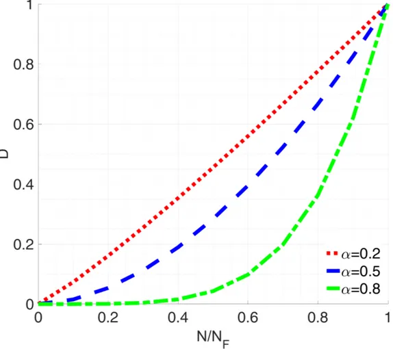
4.5 Inﬂuence of function α in fatigue damage versus fatigue life ratio (γ = 0.1) . . . 58

4.6 Inﬂuence of function γ in a plot of damage versus fatigue life ratio with α = 0.8. . . 59

4.7 AII− NF curve in rotation at r=0.1 . . . 62

4.8 Two-stress level loading in pure rotation at r=0.1. The lower curve displays the rel-ative proportion of cycles in high-low sequence, the upper curve displays the same information in a low-high sequence. . . 63

4.9 AII− NF curve in 4-point bending at y=3. . . 64

4.10 Two-stress level loading in 4-point bending at y=3. The lower curve displays the relative proportion of cycles in high-low sequence, the upper curve displays the same information in a low-high sequence. . . 65

4.11 AII− NF curve in rotative bending at r=3 . . . 65

4.12 Two-stress level loading in rotative bending at r=0.5. The lower curve displays the relative proportion of cycles in high-low sequence, the upper curve displays the same information in a low-high sequence. . . 66

4.13 Complex Cyclic Loading . . . 68

4.14 Reorder to Start from Absolute Maximum (retrieved from “How to Calculate Fatigue Life When The Load History Is Complex”, February 13, 2015, author: Michael Bak, https://caeai.com/blog/how-calculate-fatigue-life-when-load-history-complex) . . . . 69

4.15 Imagine Filling with Water and Extract Stress Range and Mean Stress (retrieved from “How to Calculate Fatigue Life When The Load History Is Complex”, February 13, 2015, author: Michael Bak, https://caeai.com/blog/how-calculate-fatigue-life-when-load-history-complex). . . 69

4.16 Drain Water Starting at Lowest Valley and Repeat Cycle Extraction (retrieved from “How to Calculate Fatigue Life When The Load History Is Complex”, February 13, 2015, author: Michael Bak, https://caeai.com/blog/how-calculate-fatigue-life-when-load-history-complex). . . 69

4.17 Rainﬂow counting method demonstration . . . 70

4.18 One million normally distributed random stresses around -100MPa . . . 70

4.19 Amplitudes distribution extracted from Figure 4.18 . . . 71

4.20 Mean stresses distribution extracted from Figure 4.18 . . . 71

4.21 Rainﬂow matrix extracted from Figure 4.18 . . . 72

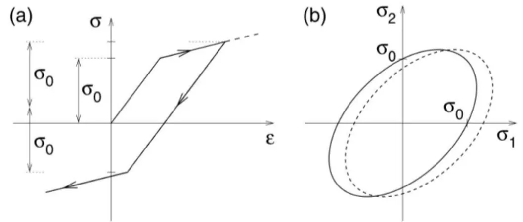
5.1 Kinematic hardening: a) uniaxial stress-strain diagram, b) evolution of the yield sur-face in the biaxial stress plane . . . 75

5.2 Haigh diagram showing test data points for the effect of mean stress, and the Gerber, modiﬁed Goodman and Soderberg relations. . . 78

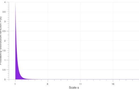
5.3 Weakening scales s probability distribution curve when β = 1.5 . . . 79

5.4 Weakening scales s probability distribution curve when β = 5 . . . 80

(12)

LIST OF FIGURES xi

5.6 Illustration of uniaxial cyclic load with microscopic plastic dissipation at scale s. With Σy = 298MPa, Σa= 190MPa, λ+= 0.9, λ− = 0. There is energy dissipation

when ||S − b||(t) projects on the local yield limit (σy− λΣH) /s(t). . . 82

5.7 The relation between ˜D and D when γ = 2 . . . 84 5.8 High to low and low to high loading sequence comparison in 4-point bending(Flow =

5000N, Fhigh = 30000N, Radius = 0.2m, Σu = 167MPa), with the proposed

dam-age accumulation law (Eq.(5.6.5)) induced equation Eq.(5.6.10) and Chaboche type α (Eq.(5.6.7)) containing Crossland criterion. . . 87 5.9 The evolution of α in bending and torsion with Σy = 1080 MPa, Σbending = Σtorsion=

500 MPa, a = 0.3 and 200 time steps in one cycle . . . 92 5.10 Comparing numerical strategy with optimal time steps in one cycle with the old one,

in this way the number of steps in unit cycle is reduced from 400 to 35, meaning a cost reduction factor of 0.0875 (with ∆α = 0.05, a = 0.4, λ = 0.1, Σy = 230 MPa,

Σbending= 225 MPa) . . . 92

5.11 S-N curve of bending test on 30NCD16 steel using numerical and analytical method (Eq.(5.7.15)) with different time steps. Data are those of table.5.1 . . . 94 5.12 S-N curve using analytical and numerical results with optimal time steps methods

(β = 1.1, a = 0.01, ∆α = 2E −5 in unit cycle), yielding 200 full time steps reduced to 197 optimal time steps . . . 96 5.13 S-N curve using analytical and numerical results with optimal time steps methods

(β = 1.1, a = 0.01, ∆α = 1E −5 in unit cycle), yielding 200 full time steps reduced to 199 optimal time steps . . . 96 5.14 Relative error

(

N Fopt− NFanalytical

N Fanalytical

)

between analytical and numerical results with optimal time steps methods (β = 1.1, a = 0.01, ∆α = 2 × 10−5_{in unit cycle)} _. ₉₇

5.15 Relative error (

N Fopt− NFanalytical

N Fanalytical

)

between analytical and numerical results with optimal time steps methods (β = 1.1, a = 0.01, ∆α = 1 × 10−5_{in unit cycle)} _. ₉₇

5.16 Microscopic(_{S − b})

trialand

(

S_{− b})evolution with time under different weakening scales (s3 = 1.21 and s10= 1.13) in sinusoidal load with zero mean stress. . . 98

5.17 Microscopic(_{S − b})

trialand

(

S_{− b})evolution with time under different weakening scales (s3 = 1.21 and s10= 1.13) in sinusoidal load with mean stress=300 MPa . . . 99

5.18 Validation of dissipated energy in all scales with analytical (method 3) and numerical method (method 1) with β = 1.1,Σ = 0.85σy. The time evolution of α does not

play a role in the dissipation calculation which is normal since α does not enter in the dissipation calculation . . . 99 5.19 Validation of dissipated energy in all scales with analytical and numerical method(enlargement

of Figure 5.18) . . . 100 5.20 Dissipated energy accumulation through time with different methods, there are 100

time steps in unit cycle . . . 100 5.21 Dissipated energy accumulation through time with of 3 methods(enlargement of

Fig-ure 5.20). . . 101 5.22 Relative difference Wanalytical− Wnumerical

Wanalytical

between analytical energy loss and nu-merical one with α varying with time of Figure 5.20. . . 101 5.23 Damage evolution with time under sinusoidal load with different methods, there are

100 time steps in unit cycle(β = 1.1,Σ = 0.85σy) . . . 102

5.24 Damage evolution with time under sinusoidal load with two different methods(enlargement of Figure 5.23) . . . 102

(13)

xii LIST OF FIGURES

5.25 Relative differenceDanalytical− Dnumerical Danalytical

evolution with time of Figure 5.23 . . . 103 5.26 Validation of dissipated energy in all scales with analytical and numerical method

with β = 5, Σ = 0.4σy . . . 103

5.27 Validation of dissipated energy in all scales with analytical and numerical method with β = 5, Σ = 0.8σy . . . 104

5.28 Damage evolution with time under sinusoidal load with β = 5, Σ = 0.4σy. In such

a severe loading and with extreme non-linearity, the simple Chaboche like formula with frozen α departs from the outcome of the full numerical model . . . 104 5.29 Damage evolution with time under sinusoidal load with β = 5, Σ = 0.8σy . . . 105

5.30 Two level sequence effect. By comparing the vertical ﬁgures we can see high stress gives high (1−α) value which causes fast damage accumulation speed. The evolution of (1 − α) is highly nonlinear and follows the value of stress at each time step. . . . 107 5.31 Fatigue life of random loading dispersion on AW-6106 T6 aluminum, test data

pro-vided by CETIM . . . 108 5.32 Major damage effect using different magniﬁcation power of Eq.(5.8.1) on sequence

effect. Here high stress is 1 MPa and low stress is 0.8 MPa. We see that using a large power f in Eq.(5.8.1) induces a stronger sequence effect. . . 109 5.33 (1-α) term which stands for the load intensity evolution, both with and without the

magniﬁcation power f . . . 110 5.34 Back stress with linear and nonlinear backstress evolution. . . 118 5.35 _{S − b} with linear and nonlinear backstress evolution. The sunken part is due to

yield limit reduction in traction. Back stress is small compared to the deviatoric stress. 118

6.1 Complex loading of a car suspension arm (data from PSA tests) . . . 120 6.2 Specimen geometry for fatigue tests of AW-6106 T6 aluminum (sample given by PSA)121 6.3 Random loading history on BATCH_A_06 of AW-6106 T6 aluminum (see Tab.6.2) . 121 6.4 Comparison between experimental and numerical results of 1D cyclic and random

loading on aluminum fatigue tests by CETIM with constant α from the ﬁrst row of Tab.6.7. . . 124 6.5 Comparison between experimental and numerical results of 1D cyclic and random

loading on aluminum fatigue tests by Cetim with load dependent α. Coefﬁcients data are given in the second row of Tab.6.7 . . . 125 6.6 Specimen geometry for fatigue tests of aluminum 6082 T6 (dimension in

millime-ters), from Susmel and Petrone [2003] . . . 126 6.7 The loading path and loading waveform of multiaxial corrosion fatigue (stress

con-trol) (a) loading path of proportional and non-proportional, (b) loading waveform of proportional loading, (c) loading waveform of non-proportion (Huang et al. [2017]) . 129 6.8 The 90◦ _{out-of-phase loading path has been found to produce the largest degree of}

non-proportional hardening (EFA). . . 129 6.9 Calibration on on 6082 T6 aluminum (Susmel and Petrone [2003]). Comparison

between experimental results and our model used with coefﬁcients given in Tab.6.11. We obtain a good correlation in bending and torsion tests. The out of phase test are not satisfactory in these batches: P32BT8, P41BT15, P36BT11. . . 130 6.10 Calibration on 30NCD16 (Dubar [1992]). We can observe that the bending-torsion

(14)

LIST OF FIGURES xiii

6.11 Calibration on 30NCD16 (Dubar [1992]). In ﬁgure (c) test 29 (same NF with test

30 but with smaller σx,m) and test 32 (2-D with large mean stress) from Tab.6.15 are

more dispersed. The numerical tests are carried out using the coefﬁcients of Tab.6.16 133 6.12 Fatigue curves on SM45C steel by Lee [2013] . . . 135 6.13 Calibration on SM45C . . . 138 6.14 Calibration on SM45C. The numerical tests are carried out using the coefﬁcients of

Tab.6.22 . . . 139 6.15 Bending-torsion fatigue tests on cylindrical specimens (Carpinteri et al. [2003]) . . . 141 6.16 Bending-torsion fatigue tests on cylindrical specimens (Carpinteri et al. [2003]) . . . 142 6.17 Multiaxial random loading sequence . . . 143 6.18 Saof bending tests with mean stress on 10HNAP . . . 145

6.19 Hydro₊₋of bending tests with mean stress on 10HNAP . . . 146 6.20 Bending and torsion test on 10HNAP steel(R=-1). Data are presented in Tab.6.30

and 6.31. The torsion best ﬁt and the bending numerical results(optimal time step of method 2 deduced in Chapter 5) are obtained with the coefﬁcients of Tab.6.28 . . . . 147 6.21 Wöhler tensile curves for various mean stress values. Data are presented in Tab.6.25

and results are obtained with the coefﬁcients of Tab.6.28 . . . 148 6.22 Calibration on 10HNAP steel, bending and torsion tests on 10HNAP(R=-1). Data are

presented in Tab.6.30 and 6.31 and results obtained with the coefﬁcients of Tab.6.28. 149 6.23 Calibration on 10HNAP steel, bending tests with various mean stress on 10HNAP,

data from Tab.6.25 and results obtained with the coefﬁcients of Tab.6.28. For the case of σm = 300 MPa, the macroscopic maximum stress is greater than yield limit, which

does not match our assumption that the material stays in elastic regime macroscopi-cally (section 5.4.1).. . . 150 6.24 Random bending-torsion 2D tests on 10HNAP, data from Tab.6.26 and Jabbado [2006].

Results are obtained with the coefﬁcients of Tab.6.29 (αM = π/8 and r = 0.2) . . . . 151

6.25 Random bending-torsion 2D tests on 10HNAP, data from Tab.6.27 and Jabbado [2006]. Results are obtained with the coefﬁcients of Tab.6.29 (αM = π/4 and r = 0.5) . . . . 152

(15)

(16)

List of Tables

3.1 Length scales of different materials. . . 44

4.1 α induced sequence effect parameter η value with different criteria in pure rotation . 63 4.2 α induced sequence effect parameter η value with different criteria in bending . . . . 64

4.3 α induced sequence effect parameter η value with different criteria in rotative bending 64 5.1 Material parameters in a simple cyclic load . . . 98

5.2 Parameters concerned . . . 112

5.3 Example of parameters sensitivity at cyclic loading of BATCH_A_02 on AW-6106 T6 aluminum (table.6.2) . . . 113

6.1 Material parameters of AW-6106 T6 aluminum . . . 120

6.2 Fatigue tests result on AW-6106 T6 aluminum, test data provided by CETIM . . . . 122

6.3 Proportion of stress above different thresholds with Σy=230MPa, test data provided by CETIM on AW-6106 T6 aluminum.. . . 123

6.4 Parameters sensitivity at random loading of ep05 on AW-6106 T6 aluminum . . . 123

6.5 Parameters sensitivity at cyclic loading of ep02 on AW-6106 T6 aluminum. . . 123

6.6 Parameters sensitivity at random loading of ep05 on AW-6106 T6 aluminum . . . 124

6.7 The parameters in 1D cyclic and random loading on AW-6106 T6 aluminum fatigue tests by Cetim . . . 124

6.8 Mechanical and dynamic characteristics of aluminum 6082 T6 (Susmel and Petrone [2003]) . . . 126

6.9 Simple bending and torsion tests (R = -1), data from Susmel and Petrone [2003] . . . 127

6.10 In-phase and out-of-phase bending-torsion tests (R = -1), data from Susmel and Petrone [2003] . . . 128

6.11 Parameter identiﬁcation of AL6082T6 . . . 128

6.12 Mechanical and dynamic characteristics of 30NCD16 steel Dubar [1992] . . . 131

6.13 30NCD16 steel fully reversed bending tests Dubar [1992] . . . 131

6.14 30NCD16 steel fully reversed torsion tests (Dubar [1992]) . . . 132

6.15 30NCD16 steel bending-torsion tests (Dubar [1992]) . . . 132

6.16 Parameter identiﬁcation of 30NCD16 steel . . . 132

6.17 Chemical composition of SM45C steel . . . 134

6.18 Mechanical and dynamic characteristics of SM45C steel . . . 134

6.19 SM45C steel fully reversed bending tests(extracted from Lee [2013]) . . . 136

6.20 SM45 steel fully reversed torsion tests(extracted from Lee [2013]) . . . 136

6.21 Effect of mean bending stress on out-of-phase(90◦_{) fatigue of SM45C steel (Lee [2013])}₁₃₇ 6.22 Parameter identiﬁcation of SM45C steel . . . 137

6.23 Chemical composition of 10 HNAP steel, data from Bedkowski [1994]. . . 140

6.24 Mechanical characteristics of steel 10 HNAP, data from Bedkowski [1994] . . . 140

6.25 Experimental results of tensile tests for various values of σm, data from Vidal . . . . 141

(17)

xvi LIST OF TABLES

6.26 Fatigue results under variable loads for α′ _{= π/8 and r = f (τ}_xy_{)/f (σ}_xx_{) = 0.2}_{. . . 142}

6.27 Fatigue results under variable loads for α′ _{= π/4 and r = f (τ}

xy)/f (σxx) = 0.5. . . 143

6.28 Model parameters for 10HNAP steel (cyclic loading) . . . 143 6.29 Model parameters for 10HNAP steel (random loading) . . . 144 6.30 Constant amplitude bending tests performed on 10HNAP steel, data from Vidal . . . 144 6.31 Constant amplitude torsion tests performed on 10HNAP steel, data from Vidal . . . . 144

(18)

(19)

(20)

Nomenclature

Σmax maximum stress during the loading cycles

Smax maximum deviatoric stress during the loading cycles

σm mean stress

σH hydrostatic stress

σ₋₁ fatigue limit for fully reversed condition s₋₁ _{tensile fatigue limit for R = −1}

b back stress

σy macroscopic yield stress

N current number of cycles

NF number of cycles to failure

˙p accumulated plastic strain rate given as√2₃_{|| ˙ε}p||

D damage variable

σa stress amplitude

σu ultimate tensile stress

⟨ ⟩ Macaulay bracket symbol which keeps

the positive value and set negative value to zero ˙

w energy dissipation rate at a certain scale ˙

W energy dissipation rate at all scales Wcyc dissipated energy per cycle

˙εp rate of effective plastic strain

˙p accumulated plastic strain rate given as√2 3|| ˙εp||

E Young’s modulus

k = 500 ∼ 800MP a hardening parameter

β weakening scales distribution exponent

γ material parameter from Chaboche law

α characterizes non-linearity of damage accumulation

a material parameter from Chaboche law

λ = 0 ∼ 3 hydrostatic pressure sensitivity S = dev ˙Σ deviatoric part of the stress tensor AII = τoct,a =

√ 1

3J2,a the amplitude of octahedral shear stress ˙εp rate of effective plastic strain

W0 reference density of damage energy

J2 The second principal invariant of the stress deviatoric tensor σV M =√3J2 Von Mises stress

(21)

(22)

Résumé en français

La recherche des meilleures performances au meilleur coût en mécanique et dans le domaine des transports conduit à des conditions d’utilisation des composants mécaniques de plus en plus sévères. Les ruptures par fatigue sont largement étudiées car elles représentent 90% de toutes les défaillances en service dues à des causes mécaniques (Sohar[2011]). Les ruptures par fatigue se produisent lorsque un métal est soumis à une contrainte répétitive ou ﬂuctuante et rompt à une contrainte très inférieure à sa résistance à la traction, et le processus se déroule sans aucune déformation plastique (pas d’aver-tissement).

Ces problèmes pratiques peuvent entraîner l’apparition de la fatigue à des niveaux très élevés de gradient de contrainte, à petite échelle ou sur des strucutures à géométrie complexe et pour des trajets de chargement multiaxiaux et non-constants. Pour ces contraintes dites "extrêmes", les mécanismes d’endommagement ainsi que les niveaux de résistance à la fatigue sont pour la plupart inconnus. Ceci pose un problème important lors de la phase de conception puisque, d’une part, les critères d’endurance existants peinent à rendre compte du comportement pour ce type de chargement, et d’autre part, les données de fatigue qui permettraient d’identiﬁer un modèle adapté à ce problème sont presque inexistantes.

D’autre part, les composants mécaniques sont généralement de nature complexe et subissent des chargements complexes. Les fabricants recherchent un modèle pour la durée de vie de leurs com-posants qui soit simple à utiliser, applicable aux matériaux métalliques et qui traite presque tous les cas de chargements possibles. Dans le domaine de l’endurance limitée, très peu de critères sont disponibles. À l’heure actuelle, aucun d’entre eux qui réponde pleinement à la demande d’un outil predictif de durée de vie ne peut être utilisé en bureau d’études. En effet, la plupart des approches existantes s’appuient sur des méthodes de comptage de cycles, dont l’extension au cas de contraintes multiaxiales s’avère difficile voire impossible en raison de la difficulté à extraire et définir des cycles. Des travaux antérieurs réalisés en collaboration avec l’entreprise PSA indiquent que les critères d’endurance multiaxiale utilisés pour les calculs de fatigue (modèle de Papadopoulos et critère de Dang Van) peinent à rendre compte efficacement de ces cas particuliers (Koutiri[2011]). Il apparait donc essentiel de caractériser les mécanismes d’endommagement pour ce type de chargement et de concevoir un modèle capable de rendre compte de ces conditions particulières de fatigue.

Ainsi, le but de cette thèse est d’établir un modèle de durée de vie déterministe pour des structures métalliques travaillant dans le domaine de l’endurance limitée à grand nombre de cycles, et qui soit capable de traiter tous les trajets de chargement (avec des amplitudes constantes et variables) sans recours au comptage de cycles.

Ce travail de thèse s’inscrit dans un projet régional de la "Chaire André Citroën", dont l’un des objectifs est de développer les aspects d’enseignement en encourageant les initiatives dans le secteur automobile et en confrontant les étudiants aux innovations technologiques typiques et aux grands déﬁs scientiﬁques. Le but de ce travail est d’étudier les critères de fatigue à grand nombre de cycles, en tenant compte des effets des changements dans le temps ou l’espace. Trois contributions ont été apportées :

(23)

2 LIST OF TABLES

- Le développement et la mise en oeuvre de méthodes d’accumulation non-linéaire de l’endom-magement.

- La mise en oeuvre d’une stratégie de mesure de la fatigue à travers une analyse multi-échelle de l’énergie dissipée, permettant ainsi de traiter des états de chargement tridimensionnels et complexes en évitant la notion de cycle de chargement.

L’étude présentée dans ce rapport se concentre plus particulièrement sur le dernier point, avec, comme nous le verrons, une attention particulière portée sur l’effet des hétérogénéités microstructu-relles sur la fatigue.

L’approche pour résoudre le problème posé comporte quatre étapes principales :

• La proposition d’une stratégie pour découpler l’effet de gradient de contrainte et l’effet de taille. •Le passage en revue des descriptions existantes des non-linéarités d’accumulation d’endomma-gement et des effets d’histoire du chard’endomma-gement.

•La construction d’un modèle de comportement à la fatigue qui rende compte des effets de la plasticité microscopique ainsi que de l’accumulation de l’endommagement et des effets de l’histoire du chargement.

• La réalisation de simulations numériques avec ce modèle, à la fois sur des conditions de char-gement cycliques et sur des trajets de charchar-gement aléatoires.

L’étude bibliographique menée dans la première partie de cette thèse (Chapitre2) vise à donner un aperçu des critères de fatigue multiaxiaux classiques et des bases physiques de leur origine. Nous comparons les modèles utilisant le concept de “elastic shakedown” avec ceux basés sur la plasticité / l’endommagement à l’échelle mésoscopique ainsi que ceux utilisant l’énergie. Nous montrerons que certains effets de chargement sont correctement représentés, mais pour d’autres, les prédictions sont très différentes d’une approche à l’autre.

La seconde partie (Chapitre3) est consacrée à l’extension de certains critères classiques de fa-tigue à grand nombre de cycle (HCF) afin de prendre en compte une sensibilité des critères aux variations spatiales de contraintes, et de comparer les performances de ces extensions à travers plu-sieurs essais expérimentaux de fatigue. L’effet bénéfique du gradient sur les essais de flexion-torsion par rapport aux essais de tension-compression est présenté. Les mécanismes des différentes approches sont comparés et une expression plus pratique et simple est proposée en tenant compte du gradient de l’amplitude de la contrainte et de la contrainte hydrostatique maximale. La généralisation de l’ap-proche à d’autres critères de fatigue multiaxiale est également proposée. Ces propositions sont ensuite testées et appliquées à différentes situations simples telles que la flexion rotative en porte-à-faux. Les erreurs relatives entre les solutions exactes et les données expérimentales sont estimées. Des essais de flexion-torsion biaxiaux sont également simulés pour démontrer les capacités de l’approche.

La non-linéarité de l’accumulation de l’endommagement est abordée dans la troisième partie (Chapitre4). L’objectif de cette section est de discuter et d’utiliser le modèle de durée de vie qui prend en compte la présence de variations complexes dans le cycle de chargement. Nous nous concentrons sur la loi d’accumulation d’endommagement de Chaboche dans le cas de la fatigue multiaxiale à grand nombre de cycle. Des formulations heuristiques avec des critères de fatigue multiaxiaux différents ont été proposées et seront brièvement passées en revue.

Le Chapitre5 considère ensuite le problème de la gestion des trajets temporels complexes en chargement multiaxial. La méthode de comptage de cycles pour comparer l’effet des historiques de chargement d’amplitude variable aux données de fatigue et aux courbes obtenues avec des cycles de charge simples à amplitude constante est présentée, ainsi que différentes approches et limitations pour le chargement multiaxial.

De ce contexte, nous développons ensuite notre nouveau modèle. Il est basé sur une description probabiliste a priori et simpliﬁée des points matériels locaux faibles. A chacun de ces points, un mo-dèle de plasticité local à écrouissage cinématique est introduit, avec une distribution donnée p(s) des

(24)

LIST OF TABLES 3

facteurs d’affaiblissement de la limite d’élasticité. Pour prendre en compte une dépendance du com-portement macroscopique en fatigue à la contrainte hydrostatique, la limite d’élasticité à chaque point local est supposée dépendre de cette contrainte hydrostatique macroscopique. Le modèle supposera alors que l’accumulation de la fatigue dépend de l’énergie dissipée par la plasticité de tous ces points au cours de l’histoire du chargement. Cette énergie, à travers toutes les échelles s, sera combinée avec les lois d’accumulation d’endommagement non-linéaires du Chapitre4 pour produire un modèle “ multi-échelles” simpliﬁé de l’évolution de l’endommagement microscopique.

Le sixième chapitre traite de la mise en uvre numérique de notre méthode et de sa validation sur différents résultats expérimentaux. Au lieu de faire l’intégration directement, ce qui peut s’avérer dif-ﬁcile pour un chargement complexe, la règle de quadrature gaussienne avec des points de Legendre est utilisée pour donner la valeur du taux d’énergie dissipée locale. Les essais cycliques et aléatoires sur l’alliage d’aluminium utilisé pour le bras de suspension automobile sont calibrés avec notre mo-dèle. Enﬁn, dans le dernier chapitre, nous faisons une application multidimensionnelle qui montre les capacités de prédiction de la durée de vie en fatigue pour différents matériaux et types de chargement.

(25)

(26)

1

Introduction

Contents

1.1 General introduction . . . 5

1.1.1 Industrial background and motivation . . . 6

1.1.2 Context and background . . . 7

1.1.3 Outline of the work . . . 7

1.1 General introduction

The fatigue of metallic structures subjected to cyclic stresses is a phenomenon which is tradition-ally studied at two levels. The fatigue is respectively qualified “low cycle" or “high cycle" if the load causing the rupture is applied during a relatively small or a large number of cycles. In turn, “high cycle fatigue" is divided in two domains: “limited endurance" where we speak of the finite lifetime regime and "unlimited endurance" where the structure can support a number of cycles theoretically infinite without breaking.

The threshold value dividing low- and high-cycle fatigue is somewhat arbitrary, but is generally based on the raw materials behavior at the micro-structural level in response to the applied stresses. Low cycle failures typically involve significant plastic deformation. An example would be reversed 90◦_{bending of a paper clip. Gross plastic deformation will take place on the first bend, but failure will} not occur until approximately 20 cycles. Plastic deformation does play a role in high cycle fatigue; however, the plastic deformation is very localized and not necessarily discernible by a macroscopic evaluation of the component. Most metals with a body centered cubic crystal structure have a charac-teristic response to cyclic stresses. These materials have a threshold stress limit below which fatigue cracks will not initiate. This threshold stress value is often referred to as the endurance limit. In steels, the life associated with this behavior is generally accepted to be 2×106_{cycles (}_Stone_[₂₀₁₂_{]). In other} words, if a given stress state does not induce a fatigue failure within the first 2 × 106 _{cycles, future} failure of the component is considered unlikely. For spring applications, a more realistic threshold life value would be 2 × 107 _{cycles (}_Stone_[₂₀₁₂_{]). Metals with a face center cubic crystal structure} (e.g. aluminum, austenitic stainless steels, copper, etc.) do not typically have an endurance limit. For

(27)

6 CHAPTER 1. INTRODUCTION

these materials, fatigue life continues to increase as stress levels decrease; however, a threshold limit is not typically reached below which inﬁnite life can be expected.

1.1.1 Industrial background and motivation

The search for the best performance at the best cost in mechanics and transport leads to increas-ingly severe conditions of use of the mechanical components. Fatigue failures are widely studied because it accounts for 90% of all service failures due to mechanical causes (Sohar[2011]). Fatigue failures occur when metal is subjected to a repetitive or ﬂuctuating stress and will fail at a stress much lower than its tensile strength and the process happens without any macroscopic plastic deformation (no warning).

These practical problems can lead to the emergence of fatigue for very high level of stress gradient for small scale or complex geometric structures and non-constant multiaxial loading history . For these so-called "extreme" stresses, the mechanisms of damage as well as fatigue resistance levels are mostly unknown. This poses an important problem during the design phase since, on the one hand, the existing endurance criteria struggle to account for behavior for this type of loading, and on the other hand, the fatigue data that would allow to identify a model adapted to this problem are almost non-existent.

On the other hand, the mechanical components are generally of complex nature undergoing com-plex loads. Manufacturers are looking for a model of lifetime of their components, which is simple to use, great applicability to metallic materials and which treats almost all cases of possible loads. In the domain of limited endurance, very few criteria are available. At present, none of them can be used in design offices, and does fully meet the demand for predictive tool for lifetime. Indeed, most of the existing approaches rely on methods of counting cycles, whose extension to the case of multiaxial stresses turns out to be difficult or even impossible because of the difficulty of extracting and defining cycles.

Previous work carried out in collaboration with the PSA company indicates that the criteria of multi-axial endurance used for fatigue design (Papadopoulos model and Dang Van’s criterion) strug-gle to account effectively for these very speciﬁc cases (Koutiri[2011]). It therefore seems essential to characterize the mechanisms damage of this type of loading and to implement a modeling able to reﬂect these particular fatigue conditions.

The aim of this thesis is thus to establish a deterministic model of lifetime on metal structures working in limited endurance in high cycle fatigue, which handles almost all load cases (with constant and variable amplitudes) without recourse to cycle counting.

This thesis work is part of a regional project of "Chaire André Citroën"; one of whose objectives is to develop teaching by encouraging initiatives in the automotive sector and confronting students with typical technological innovations and major scientiﬁc challenges. The aim of this work is to study the fatigue-related criteria with a large number of cycles, taking into account the effects of variation in time or space. Three contributions were developed:

- Extension of the fatigue criteria to take into account the gradient effect. - Development and testing of nonlinear accumulation methods of damage.

- Implementation of a strategy for measuring fatigue through a multi-scale analysis of the dissi-pated energy, thus enabling three-dimensional and complex states of charge to be treated and avoiding the notion of loading cycle.

The study presented in this report focuses more particularly on the last theme, with, as will be seen, a particular emphasis on the effect of micro-structural heterogeneities on fatigue.

The approach for solving the problem posed has four main stages:

(28)

1.1. GENERAL INTRODUCTION 7

• Review of the existing description of the non-linearity of damage accumulation and history dependent sequence effects.

• Construction of a model of fatigue behavior that accounts for the effects of microscopic plastic-ity as well as damage accumulation and history sequencing effects.

• Numerical simulation with such a model both on cyclic loading conditions and on random loading history.

1.1.2 Context and background

The fatigue of materials with many cycles is one of the phenomena that can lead to rupture of machine parts or structures in operation. Its progressive character masked until sudden breakage does not allow easy prediction of the durability of the structure.

The main factors influencing the fatigue resistance of materials are numerous (loading mode, temperature, micro-structural heterogeneities, residual stresses ...), making it a complex phenomenon to study. A lot of work has been done in the goal of better understanding the influence of these different factors. One of the main parameters influential, repeatedly studied, is the damage mechanism of the time varying stress.

Numerous experimental observations made on metallic materials have shown that the damage mechanisms operating in fatigue with large number of cycles and leading to breakup are of two cat-egories. In a first step known as the priming step, micro-plasticity mechanisms, generally operating around heterogeneities specific to the material (inclusions, porosities, etc.), are the origin of the ap-pearance of micro-cracks. If the load level is high enough, these cracks increase and cross a number of micro-structural barriers (e.g. grain boundaries). When the crack has reached a size sufficiently large in relation to the plasticized zone, a second phase intervenes where it propagates according to, the laws of fracture mechanics.

Two types of very distinct approaches are often used to model these mechanisms. The ﬁrst con-cerns initiation and mainly uses the framework of the mechanics of the micro-plasticity considered to be the main cause of onset of a crack. The second uses the fracture mechanics framework to estimate the number of cycles necessary for the propagation of a pre-existing crack (Koutiri[2011]).

In our work we concentrate on the ﬁrst phase and consider the mechanisms related to the stochas-tic distribution of pre-existing micro-cracks at different scales which undergo strong plasstochas-tic yielding in cyclic load history. The number of cycles to failure is determined from the plastic shakedown cycle occurring at these microscales.

1.1.3 Outline of the work

The bibliographical study conducted in the ﬁrst part of this thesis (Chapter2) aims to overview the basic multiaxial fatigue criteria and the physical basis of their origin. Models using the elastic shakedown concept, plasticity / damage on the mesoscopic scale as well as energy are compared. We will show that some loading effects are correctly reﬂected, however for others, the predictions are very different from one approach to another.

The second part (Chapter3) is devoted to the extension of some classic high cycle fatigue (HCF) criteria in order to take into account a sensitivity of the criteria to stress spatial variations, and sec-ond to compare the performances of the extensions through several experimental fatigue tests. The gradient beneﬁcial effect on bending-torsion in comparison with tension-compression is presented. Different approaches are compared and a more practical and simple expression is proposed taking into account the gradient of the stress amplitude and the maximum hydrostatic stress. The general-ization of the approach to other multiaxial fatigue criteria is also proposed. The proposition is then tested and applied to different simple situations such as cantilever rotative bending. The relative errors

(29)

8 CHAPTER 1. INTRODUCTION

between the exact solutions and the experimental data are estimated. Biaxial bending-torsion tests are also simulated to demonstrate the capabilities of the approach.

The non-linearity of damage accumulation in fatigue is discussed in the third part (Chapter4). The objective of this section is to review and use the developed life model that takes into account the presence of complex variations of the load cycle. We focus on Chaboche damage accumulation law in case of multiaxial high cycle fatigue. Heuristic formulations with different multiaxial fatigue criteria have been proposed and will be brieﬂy reviewed.

Chapter5then considers the problem of handling complex time histories in multiaxial loading. Cycle counting method to compare the effect of variable amplitude load histories to fatigue data and curves obtained with simple constant amplitude load cycles is presented, together with different approaches and limitations for handling multiaxial loading.

From this context, we then develop our new model. It is based on a probabilistic description of local material weak points. At each such point, a local plastic model with kinematic hardening is introduced, with a given distribution p(s) of yield weakening factors. To take into account a depen-dence of the macroscopic fatigue behavior to the hydrostatic stress, the yield limit at each local point is supposed to depend on this macroscopic hydrostatic stress. The model will then suppose that the fatigue accumulation depends on the energy which is dissipated by plasticity of all these points dur-ing the loaddur-ing history. This energy through all scales s will be combined with the nonlinear damage accumulation laws of chapter4to produce a simpliﬁed “multiscale” model of microscopic damage evolution.

The sixth chapter of the document deals with the numerical implementation of our method and its validation on different experimental results. Instead of doing the integration directly which can be difﬁcult for complex loading, the Gaussian Quadrature rule with Legendre points is used to give the value of local dissipated energy rate. Cyclic and random tests on aluminum alloy used for automobile suspension arm is calibrated with our model. Then in the last chapter a multidimensional application is performed showing the capability of prediction on fatigue life of different material and loading patterns.

(30)

2

Fatigue life calculation methods

Contents

2.1 Basquin curve . . . 9

2.2 Basic fatigue criteria . . . 11

2.2.1 Criteria based on stress . . . 12

2.2.2 Criteria based on energy . . . 17

2.2.3 Criteria based on plasticity-damage coupling . . . 22

2.3 Calculation method without cycle counting . . . 25

2.3.1 Morel’s method . . . 25

To obtain a better knowledge of the impact of different types of stresses and mechanism of en-ergy dissipation in high cycle fatigue(HCF), many researchers have carried out tests often difﬁcult to implement and to control. From the data obtained and sometimes from the observations of the associ-ated mechanisms, they have developed models that account more or less faithfully for the experiment. The approaches used are quite varied, but since the ﬁeld of fatigue that interests us (HCF) is often governed by crack initiation, we make the choice in this chapter to treat only models established in the framework of continuum mechanics. It will therefore be a question of the state of the art of the most successful existing models but above all we will try to compare the predictions obtained when dealing with the equivalent stress and energy dissipation. This study will make it possible to reveal the great variety of the predictions obtained and to direct our work towards a better understanding of the behavior for the loads appearing the most problematic.

2.1 Basquin curve

Stress-Life Diagram (S-N Diagram)

The basis of the Stress-Life method is the Wohler S-N diagram. The S-N diagram plots nominal stress amplitude S versus cycles to failure N. There are numerous testing procedures to generate the required data for a proper S-N diagram. S-N test data are usually displayed on a log-log plot, with the actual S-N line representing the mean of the data from several tests.

(31)

10 CHAPTER 2. FATIGUE LIFE CALCULATION METHODS

Figure 2.1 – Idealized S-N curve for high cycle fatigue.

Certain materials have a fatigue limit or endurance limit which represents a stress level below which the material does not fail and can be cycled inﬁnitely. If the applied stress level is below the endurance limit of the material, the structure is said to have an inﬁnite life. This is characteristic of steel and titanium in benign environmental conditions. A typical S-N curve corresponding to this type of material is shown in Figure2.1.

Many non-ferrous metals and alloys, such as aluminum, magnesium, and copper alloys, do not exhibit well-defined endurance limits. These materials instead display a continuously decreasing S-N response. In such cases a fatigue strength Sf for a given number of cycles must be specified. An effective endurance limit for these materials is sometimes defined as the stress that causes failure at 1 × 108or 5 × 108_{loading cycles.}

The concept of an endurance limit is then used in infinite-life or safe stress designs. The possi-bility of infinite cycling is due to interstitial elements (such as carbon or nitrogen in iron) that pin dislocations, thus preventing the slip mechanism that leads to the formation of microcracks. Care must be taken when using an endurance limit in design applications because infinite cycling poten-tiality can disappear due to:

• Periodic overloads (unpin dislocations)

• Corrosive environments (due to fatigue corrosion interaction) • High temperatures (mobilize dislocations)

The endurance limit by itself is not a true property of a material, since other significant influences such as surface finish cannot be entirely eliminated. However, a test values (S′

e) obtained from pol-ished specimens provide a baseline to which other factors can be applied. Inﬂuences that can then affect the endurance limit include:

• Surface Finish • Temperature • Stress Concentration • Notch Sensitivity • Size • Environment Power Relationship

(32)

2.2. BASIC FATIGUE CRITERIA 11

in Figure2.1. Basquin’s equation is a power law relationship as Eq.(2.1.1) which describes the linear relationship between the applied stress cycles (S) in the y-axis and the number of cycles to failure in the x-axis plotted on a log-log scale.

N = BS1b (2.1.1)

To calculate the slope of the Basquin equation from two signiﬁcant curve points, we need to solve the system of equations: N1= N2 ( S1 S2 )1 b , yielding b = logS1− logS2 logN1− logN2 ,

where b is the slope of the line. Then the coefﬁcient B in Eq.(2.1.1) is given by B = N1S− 1 b 1 = N2S− 1 b 2 , with S1denoting the stress range value of the considered test.

For the constant B, in industry the stress range value (from the maximum cyclic stress to the minimum cyclic stress) is often considered. If the stress values of the S-N curve are given as alter-nating stresses (which is the common practice), multiply these stresses by 2 to calculate the constant B (stress range = 2* alternating stress, assuming a zero mean stress and full reversal of the cyclic load). If the S-N curve data are given in stress range values, apply them directly in the equation for estimating the constant B.

The power relationship is only valid for fatigue lives that are on the design line. For ferrous metals this range is from 1 × 103 _{to 1 × 10}6 _{cycles. For non-ferrous metals, this range is from 1 × 10}3 _to 5 × 108cycles.

Basquin curves are quite simple but how can we apply them to more complex loadings?

This limitation is at the origin of the development of more detailed criteria to be described in the next section.

2.2 Basic fatigue criteria

This bibliographic chapter reviews different methods to calculate the lifetime of multiaxial high cycle fatigue. In fact, the difﬁculty of deﬁning the equivalent stress in situations with multiaxial loading and variable amplitude loading reveals the necessity of study these methods. These criteria allows to determine whether the stress trajectory in the stress space leads to the failure of the points concerned.

Papadopoulos suggested, in particular, to group families of fatigue criteria into four categories: • Criteria based on strain

• Criteria based on stress • Criteria based on energy

• Criteria based on plasticity-damage coupling.

Generally, the criteria developed in strain and sometimes in energy are adapted to the oligocyclic fatigue where the tests are often carried out with imposed strain. Approaches in stress and sometimes in energy, as well as those based on the coupling of plasticity and damage which have begun to emerge in recent years are being applied in the domain of endurance. Therefore, we will focus on the last three categories and analyze the different approaches.

(33)

2.2.1 Criteria based on stress

Three types of approach can be distinguished: • Critical plan approaches

• Approaches based on stress invariants

• The criteria based on mean stress in an elementary volume

For simplicity and to avoid too costly identification procedures of fatigue data, criteria are often expressed using two parameters to characterize the local load. The first relates generally to a shear stress (on a plane or on average over an elementary volume) while the second reflects the normal stress effects (mean and amplitude) through the hydrostatic stress or the normal stress. The criteria using the hydrostatic stress are the most numerous (Crossland[1956],Sines [1959],Morel [1998], Thu[2008]). The micro-macro approach applied to the field of endurance was born with the work of (Dang Van[1973]), and since it has been used many times, including by (Papadopoulos[1993]) to take better account of loading path effects.

Many fatigue limit criteria can thus be written as:

f (τ ) + g(σ) ⩽ 0 (2.2.1)

where f and g are given functions of the shear stress τ and of the normal stress σ respectively, as applied to different interfaces within the material.

The normal and shear stress acting on the material planes and used in Eq.(2.2.1) are sometimes deﬁned from a critical plane (Findley[1959a]), or through integration at every plane of an elementary volume (Liu and Zenner[1993]). Thu[2008] proposes, in particular, a probabilistic approach based on this type of integration.

Crossland Criterion

Using traditional fatigue criteria, a near hyperbolic relationship between stress and fatigue life is assumed, with an asymptotic limit deﬁned as the endurance stress. To predict this asymptotic limit, the Crossland Criterion is probably the most widely known. Crossland proposed that the second invariant of the deviatoric stress tensor and the hydrostatic pressure are the variables governing the endurance limit.

The classical Crossland criterion deﬁnes the fatigue limit of metallic specimens subjected to multi-axial in-phase cyclic stress (Crossland[1956]) :

f (√J2,a, Pmax) = τeq+ aPmax− b ⩽ 0 (2.2.2) where τeq = √J2,a measures the amplitude of variation of the second invariant of the de-viatoric stress and Pmax is the maximum hydrostatic stress observed during a loading cycle. If f (√J2,a, Pmax) is negative or null, there is no damage. If f (√J2,a, Pmax) is positive, there is likely to be damage and hence limited endurance. The physical constants a and b are material constants that needs to be determined experimentally. The amplitude of the square root of the second invariant of the stress deviator can be deﬁned, in general case, as the radius of the smallest hypersphere of the deviatoric stress path (Papadopoulos et al.[1997]):

√ J2,a= 1 √ 2minS1 { max t ( (S(t) − S1) : (S(t) − S1) )} . (2.2.3)

Recall that the deviatoric stress S associated to a stress tensor σ is deﬁned by

(34)

The maximum value that the hydrostatic stress reaches during the loading cycle is on the other hand:

Pmax = max t {

1

3tr(σ(t))}. (2.2.5)

For a proportional cyclic loading, if one introduces the two extreme stress tensors σA _{and σ}B observed during the loading path, together with the stress amplitude

∆σ = σB_{− σ}A (2.2.6)

and its deviatoric part ∆s, the variation of the second invariant of the stress deviator reduces to √ J2,a= 1 2√2maxt √ ∆s : ∆s = 1 2√2maxt √ (∆s2 11+ ∆s222+ ∆s233+ 2∆s212+ 2∆s213+ 2∆s223). (2.2.7)

The physical constants a and b can be related to the limit τ₋₁of endurance in alternate pure shear with Pmax = 0, ∆s =    0 2t 0 2t 0 0 0 0 0   

and to the limit f₋₁of endurance in alternate pure traction and compression where there is Pmax= 1 3f, ∆s =    4 3f 0 0 0 ₋2₃f 0 0 0 ₋2₃f    by a = (τ−1− f_√−1 3) f−1 3 , b = τ₋₁. (2.2.8)

Thus the classical Crossland criterion can be written as: √

J2,a+ aPmax− b ⩽ 0. (2.2.9)

with a and b given by Eq.(2.2.8). Dang Van Criterion

In multiaxial fatigue with large number of cycles, the important role of local plasticity on the appearance of a fatigue limit is widely accepted and fully justifies the use of a multi-scale approach. Among the existing approaches, one of the most known and used is that ofDang Van[1999]. This criterion is used in particular in the design of certain automotive structures at PSA and Renault. The criterion (Dang Van et al.[1986]) belongs to the family of critical plane type approaches. The main physical basis of this criterion focuses on the theory of elastic shakedown at two scales, mesoscopic and macroscopic. The macroscopic behavior of the material often remains elastic, only a grain ori-ented unfavorably undergoes plastic deformation. The author states the following hypothesis: “ The multiscale approach is settled on the assumption that under high cycle fatigue loading, a structure will not be fractured by fatigue if an elastic shakedown is reached at the macroscopic scale as well as at mesoscopic scale." (Dang Van[1999]). The approach developed first is to describe the plasticity across the grain, assuming a yield criterion. The yield criterion is the law of Schmid with a linear isotropic hardening. The author then search the elastic adaptation formula and defines a fatigue test locally as shown in Figure2.2(∆ represents the tensor defining the orientation of the sliding system,

(35)

Figure 2.2 – Elastic adaptation at the two scales (Dang Van[1999])

γ is the plastic slip and τ is the amplitude of shear stress on the deﬁned plan). Finally, a micro to macro upscaling strategy is applied to determine the criteria on the macroscopic scale. The local-ization law which is used is Lin-Taylor model that assumes equality of deformations at two scales. Using empirical relationships, the harmful role of the mean stress on the fatigue strength of the ma-terial is shown for type of uniaxial tensile stress. Dang Van shows the effect of the mean stress with hydrostatic stress term in the criteria expressed as a linear combination of mesoscopic shear stress on the maximum shear plane τaand the hydrostatic stress ΣH.

The resulting Dang Van criterion presented inBallard et al.[1995] is expressed as:

max n { max t {τa(n, t) + aDΣH(t)} } ⩽bD. (2.2.10)

where τadenotes the mesoscopic shear stress amplitude and is obtained from a mesoscopic stress tensor ˆσdeﬁned by:

ˆ

σ(t) = (σ(t)_{− s}⋆).

Here s⋆_{is the center of the smallest hypersphere circumscribed to the loading path in deviatoric stress} space. It is obtained by solving a “min-max" problem as follows:

s⋆ = arg min s₁ { max t ∥ s(t) − s1 ∥ } .

In the case of fully reversed loading, the values s⋆ _{= 0 can be directly deduced without solving the} “min-max problem" as in general case.

The principal stress values of stress tensor ˆσ being denoted by ˆσIII(t) ⩽ ˆσII(t) ⩽ ˆσI(t), one gets the amplitude of shear stress by:

max

n τa(t) = 1

(36)

Here ΣH(t)is the hydrostatic stress as a function of the time, given by: ΣH(t) =

σkk(t) 3 . The Dang Van criterion then writes

1

2(ˆσI(t) − ˆσIII(t)) + aD tr(σ)

3 ⩽bD. (2.2.11)

The material characteristic parameters aD and bD of the Dang Van criterion, can be related to the fully reversed bending or tension- compression fatigue limit because of the same stress state between them, denoted by f₋₁(or s₋₁), and to the torsion fatigue limit, denoted by τ₋₁,

aD = 3τ₋₁ s₋₁ − 3 2; bD = τ−1.

In the particular case of the uniaxial tension with average load Σxx,m and amplitude Σxx,a, the criterion is written as:

Σxx,a ( 1 2+ aD 3 ) + Σxx,m (aD 3 ) = bD. Papadopoulos Criterion

The approach proposed byPapadopoulos[1993] also uses the concept of elastic adaptation and even the localization law. According to him, “the observations at the mesoscopic scale show that the initiation of a fatigue crack is deﬁned as the occurrence of micro-cracks corresponding to the rupture of the most deformed crystal grains in an aggregate. Thus, a fatigue limit criterion can be modeled by a limit value of the accumulated plastic strain in the most distorted grain."

γcum⩽γ∞.

He proposes to opt for a mean value of the accumulated plastic strain on all possible slip systems of representative elementary volume (REV). So he chose to use a average value of accumulated plastic deformation rather than looking at failure of a single crystal. A spherical coordinate system is shown in Figure2.3 to guide the normal vector in the material plane, and the unit direction vector r linked to a sliding direction of this plan is used to conduct the integration over all possible orientations.

More precisely, at any point O of a body, a material plane ∆ can be deﬁned by its unit normal vector n. This vector n makes an angle θ with the z-axis of a Oxyz frame attached to the body, and its projection on the xy plane makes an angle φ with axis x. For each plane ∆ a new quantity is introduced called generalised shear stress amplitude and denoted as Ta.This shear stress quantity was ﬁrst introduced inPapadopoulos [2001] and was subsequently used by other researchers.The critical plane according to our proposal is that onto which Ta(φ, θ) achieves its maximum value. The fatigue limit criterion is written as:

maxTa+ α_∞Σh,max ⩽γ∞ (2.2.12)

where α_∞and γ_∞ are material parameters to be determined (Papadopoulos[2001]), and where we take Σh,max = max t { 1 3tr(σ(t)) }

(37)

Figure 2.3 – Material plane ∆ passing through point O of a body and its associated (n, l, r) frame(Papadopoulos[1993]).

To deﬁne Ta, he introduced the resolved shear stress τ:

τ =[sinθcosφσxx+ sinθsinφσxy+ cosθσxz](−sinφcosχ − cosθcosφsinχ)+ [sinθcosφσxy+ sinθsinφσyy+ cosθσyz](cosφcosχ − cosθsinφsinχ)+ [sinθcosφσxz+ sinθsinφσyz+ cosθσzz]sinθsinχ.

(2.2.13)

It is clear that the resolved shear stress is a function of φ, θ, χ and of time t in the case of variable loading, i.e. τ = τ(φ, θ, χ, t). Upon ﬁxing a couple (φ, θ) (i.e. a plane ∆) and an angle χ (i.e. a line ξ on ∆), one can deﬁne the amplitude of the resolved shear stress τa, acting on ∆ along ξ by the formula: τa(φ, θ, χ) = 1 2 [ max t∈P τa(φ, θ, χ, t) − mint∈P τa(φ, θ, χ, t) ] . (2.2.14)

Finally, for a given plane ∆, i.e. for a ﬁxed couple (φ, θ), the generalized shear stress amplitude Ta is deﬁned as: Ta(φ, θ) = √ 1 π ∫ 2π χ=0 τ2 a(φ, θ, χ)dχ (2.2.15)

We note the fatigue limit in fully reversed torsion τ₋₁ and the fatigue limit in fully reversed bending f₋₁. From these two tests we get the parameters:

γ_∞= τ₋₁, α_∞= 3 ( τ₋₁ f₋₁ − 1 2 ) .

The Papadopoulos fatigue limit criterion achieves the form (Papadopoulos[2001]):

maxTa+ 3 ( τ₋₁ f₋₁ − 1 2 ) Σh,max⩽τ−1. (2.2.16)

(38)

In the particular case of the fully reversed uniaxial tension, the criterion is written as (Papadopoulos [2001]):

Σxx,a 2 + α∞

Σxx,m 3 ⩽γ∞

In conclusion of this part in stress based criteria, we need to observe that these criteria are all based on the notion of cyclic loading, which can be a limitation in general case.

2.2.2 Criteria based on energy

Depending on the type of density of deformation energy considered per cycle, the Energy criteria are divided into three groups (Macha and Sonsino[1999]):

• criteria based on elastic energy • criteria based on plastic energy

• criteria based on the sum of elastic and plastic energies.

The criteria based on the elastic deformation energy can be used in fatigue with a large number of cycles, whereas those based on the plastic deformation energy are more suitable for oligocyclic fatigue.

Ellyin[1974] is one of the ﬁrst to propose a fatigue criterion based on cyclic shear deformation energy. This approach was taken up and complemented byLefebvre[1981] andEllyin et al.[1991] for the case of multiaxial loadings. In France, this approach is reﬂected in the work ofFroustey et al. [1992] and then inPalin-Luc[1996] andBanvillet[2001].

Energy dissipation based on strain energy density

In their fatigue criterion,Froustey et al.[1992] have considered a complete cycle of stresses. They use the mean value on one cycle of the volumic density of the elastic strain energy, Wa, whatever the point M in the mechanical part.

Wa(M ) = 1 T ∫ T 0 1 2σij(M, t)ε e ij(M, t)dt

where σij(M, t) and εeij(M, t) are respectively the tensor of stresses and the tensor of elastic strains at the considered point M function of time t. Thus, in low cycle fatigue Wacan be considered as the mean value on one cycle of the total strain energy density at the considered point. However, in high cycle fatigue usually the endurance limit is low enough to consider that the material remains elastic at the macroscopic scale (Chaboche and Lesne[1988a]).

In 1998 Thierry PALIN-LUC and Serge LASSERRE (Palin-Luc and Lasserre[1998]) proposed a failure criterion based on Wa. Their studies show that another limit, called σ∗, can be deﬁned below the usual endurance limit of the material, σD. At a considered point a stress amplitude below this new limit does not initiate observable damage at the microscopic scale (no micro-cracks). Two static characteristics of the material are necessary: E and ν. Three experimental endurance limits under fully reversed loadings are needed: the endurance limit in traction,σD

T rac,−1, the endurance limit in rotative bending, σD

RotBend,−1, and the endurance limit in torsion, τT o,−1D .

This stress limit σ∗ _{can be estimated from fatigue test results in fully reversed tension and in} rotating bending

σ∗ ₌√_2(σD

(39)

From σ∗_{and by analogy with a sinusoidal traction load the corresponding mean value of the strain} energy volumetric density, Wa∗, can be calculated , where E is the Young modulus of the material.

Wa∗=

σ∗2 4E.

Around each point it is always possible to deﬁne the volume V∗_(C_i_{) by the set of points M where} Wa(M ) is higher than Wa∗(C_i) . They postulate that the part of W_a(M ) exceeding W_a∗(C_i) is the

damaging part of the strain energy volumetric density. They thus calculate ωa(Ci) the volumetric mean value of the strain energy around the critical point Ci

V∗_(C

i) = {points M(x, y, z) around Ci such that Wa(M ) ⩾ Wa∗(C_i)}

ωa(Ci) = 1 V∗_(C_i₎ ∫ ∫ ∫ V∗_(C_i₎ [Wa(x, y, z) − Wa∗(C_i)]dν

At the endurance limit and at the critical point Ci, this new quantity ωa(Ci) is supposed to be constant, whatever the uniaxial stress state. If we note ωD

a(U niax) its value at the endurance limit for any uniaxial stress state our criterion can be written by Eq.(2.2.17). Failure occurs if this equation is not veriﬁed.

ωa(Ci) ⩽ ωDa(U niax). (2.2.17)

The limitation of this criterion is that it only deals with constant amplitude load case.

A critical plane approach based on energy concepts

Łagoda et al.[1999] proposed that under multiaxial loadings the normal strain energy density in the critical plane (i.e. the plane of the maximum damage) to be the energy parameter and translated into deformation or stress amplitude in a given experimental fatigue curve. The history of strain energy density is schematized with use of the rain-ﬂow algorithm. Fatigue damage is accumulated according to Palmgren-Miner hypothesis and endurance limit uses the standard fatigue characteristic of the material, rescaled with use of the considered energy parameter.

W (t) = 1

2σ(t)ε(t)sgn[σ(t), ε(t)] (2.2.18)

sgn(x, y) = sgn(x) + sgn(y) 2

sgn(x), sgn(y) = 0, 1, −1 for distinguishing positive and negative works in a fatigue cycle. Thus, it allows to distinguish energy (speciﬁc work) for tension and energy (speciﬁc work) for compression. If the stress and strain reach their maximum values, σaand εa, then the maximum energy density value is

Wa= 1

2σaεa (2.2.19)

Taking W (t) as the fatigue damage parameter according to Eq.(2.2.18), we can rescale the stan-dard characteristics of cyclic fatigue (σa− NF) and (εa− NF) and obtain a new one, (Wa− NF ). In the case of high-cycle fatigue, when the characteristic curve (σa− NF) is used in order to predict the number of cycles NF to failure, the axis σashould be replaced by Wa, where Waand σaare related by:

Wa= σ2

a 2E.