Do French Low-Income GPs Choose to Work Less ?

Cahiers de la Chaire Santé

Low-income self-employed GPs: a

preference for leisure?

Auteur : Anne Laure Samson

Low-income self-employed GPs: a preference for

leisure?

Anne-Laure Samson

July 6, 2010

Abstract

In France, each year between 1993 and 2004, 5 to 7% of general practitioners (GPs) earn less than 1.5 times the level of the French minimum wage. This article examines who are those low-income GPs using a representative panel of French self-employed GPs over the years 1993 to 2004. We …nd that experiencing low incomes, even during a short period of time, has a lasting impact on GPs’ incomes over their whole career. Low-income GPs are mainly female or physicians practicing in areas where medical density is high but where the quality of life is also better. To test if low incomes result from a preference for leisure (ie if low-income GPs choose to work less than all other GPs or if they are constrained to), the econometric analysis consists of measuring GPs’ reaction to a shock of demand. We show that low-income GPs never react to an increase in demand, while it would give them the opportunity to increase their activity and their incomes. They only react to negative shocks of demand, i.e. they decrease their activity when they are constrained to. Conversely, all other GPs always react to

I thank, for their useful comments and suggestions, Brigitte Dormont, Eve Caroli, Pierre-Yves Geo¤ard, Agnes Gramain, Alain Trannoy, participants at the Paris Dauphine and Paris 1 seminars and participants at the Journées des économistes de la santé and AFSE conference (2009).

y_{LEDA-Legos, Université Paris Dauphine, France. Tel : 0033-1-44 05 46 33. E-mail :}

positive and negative shocks of demand : their activity is strongly constrained by the demand they are facing. We conclude that low-income GPs are physicians who choose to work less : to respond to the increasing demand by increasing their activity would reduce their utility. Their low incomes do not re‡ect a downgrading of the GPs’ profession, but rather one of its advantages: as self-employed, GPs can freely choose their number of hours of work. They may choose to work less.

JEL Classi…cation: I12, J22, C23

Keywords: labour supply, labour-leisure trade-o¤, GPs, self-employed, target in-come, longitudinal data

1

Introduction

Standard models of labour supply always make the asumption that workers freely decide the number of hours they want to work (Blundell and MaCurdy, 1999). This asumption is obviously wrong when one analyses labour supply of salaried workers. However, one kind of profession is not subject to this criticism : the self-employed professionals. Litterature about self-employed professionals in general is very scarce. Pioneering work was performed in 1945 by Friedman and Kuznets (1945) who compared physicians’ incomes with other professionals (lawyers, dentists). Lazear and Moore (1984) studied careers of self-employed professionals using cross-sectional data. More recently, Ajayi-Obe and Parker (2005) compared earnings of British self-employed professionals and employees using longitudinal data. The small literature on self-employed workers is mainly due to the lack of reliable data on these professionals.

Recently, some studies have concentrated on the labour supply of self-employed pro-fessionals, focusing on the idea that these workers’ behaviours could be driven by a "target-income". In the US, one profession received particular attention, the cab drivers. Camerer et al. (1997) study the daily hours of New-York City cab drivers. They show that these drivers, who can control their number of hours of work, stop working once they have reached their target daily income but work longer on days when they have few

customers. They …nd a negative elasticity of daily hours of work with respect to income. They conclude that this behaviour is consistent with a target income hypothesis. How-ever, their study is subject to econometric biaises, that are not treated. More recently, Farber (2005), using other data on New-York City cab drivers and another methodol-ogy refutes this conclusion : the probability of stopping work is more in‡uenced by the cumlulative hours worked on a day than by the cumulative income earned.

The target-income hypothesis has been widely criticized in health economics, as shown by Folland et al. (1997). In particular, McGuire and Pauly (1991) raise several criticism towards this hypothesis : why would doctors stop their activity as soon as they reach a certain level of activity? How are the targets de…ned? How di¤erences in targets between physicians can be explained? All these questions are still unanswered. Very few empirical studies have been able to prove the existence of a target-income among physicians. The most recent studies are from Rizzo and Zeckhauser (2003, 2007) who use US data relative to young physicians in which they observe a "reference income" (a declared income: the income physicians consider as adequate given their career stage). Rizzo and Zeckhauser (2003) show that the reference income has a much smaller impact on the log of annual incomes of physicians who are above there reference income (+0.13) than on those who are below (+0.59). In a more recent article, Rizzo and Zeckhauser (2007) show that male and female respond di¤erently to their reference income : male respond strongly when their incomes fall below their reference income (by reducing the lenght accorded to each encounter), but female activity is insensitive to this reference income.

In this paper, I focus on one kind of self-employed professionals: General Practitioners (GPs). This study reopens the debate on the existence of a target income for self-employed professionals by revealing high income disparities among French GPs. In France, most GPs are self-employed and are paid through a fee-for-services scheme. Reference fees are …xed for each service by a bargaining between the public health insurance and medical associations. GPs’incomes are therefore closely related to their

level of activity and the number of hours they work.

While average GP’s incomes are high (5 000e in 2004), there is a huge heterogeneity in incomes between GPs, especially at the bottom of the distribution. Each year between 1993 and 2004, 5 to 7% of GPs earn less than 1.5 net SMIC (the French minimum wage). The purpose of this paper is to characterize those low-income GPs: do they choose to work less than all other GPs or are they constrained to? In other words, do they have a lower optimal level of activity and a higher preference for leisure than all other GPs? We use a representative panel of more than 4,000 self-employed GPs practicing in France between 1993 and 2004. It is drawn from an administrative …le on self-employed physicians collected by the public health insurance.

This paper proceeds as follows. Section 2 describes the data, the French regulation of ambulatory care and its impact on GPs’ incomes. Section 3 describes the main characteristics of low-income GPs. Section 4 presents the microeconometric test used to check if low-income GPs choose to work less than all other GPs and gives the main empirical results. Finally, section 5 discusses the results and concludes.

2

The French regulation of ambulatory care and

GPs’earnings

2.1

The French market for ambulatory care

In France, physicians providing ambulatory care are general practitioners (GPs) or specialists, both of them being either self-employed or salaried physicians. GPs account for 45% of all physicians. 84% of them are self-employed and paid through a fee-for-services scheme. The other are salaried doctors. For self-employed GPs, reference fees are …xed for each service by a bargaining between the public health insurance and medical associations. More precisely, self-employed GPs can belong to two sectors: the

"sector 1" in which overbilling is forbidden and the "sector 2" in which it is authorized. Currently, 87% of them belong to the sector 1 and are paid the reference fees. 90% of GPs are exclusively self-employed GPs, i.e they have no salaried or hospital activity besides their self-employed activity.

As fees are …xed, GPs’incomes are closely related to their level of activity (their number or o¢ ce visits, home visits, surgery or radiology acts). Compared to other existing kinds of payment systems (capitation, salary or mixed), this system creates great incentives for a GP to increase his level of activity in order to increase his income. To increase his income, a GP can work longer or shorten the duration of visits.

2.2

The dispersion of GPs’net earnings

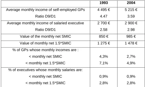
Overall, GPs’ net incomes are high (around 5,000e per month in 2004) which make them lie at the top of the distribution of incomes of all French workers. If we compare GPs’ remuneration to the remuneration of salaried top executives, we …nd that GPs’ incomes are much higher than executives’1 _{(table 1). However, income disparities are} also much pronounced among GPs. As an example, in 2004, the inter-decile ratio D9/D1 was 3.6 for GPs but only 3 for executives. This higher dispersion for GPs comes from a higher variation in incomes at the bottom of the distribution of GPs’incomes. Indeed, each year between 1993 and 2004, 5 to 7% of GPs earn less than 1.5 times the level of the legal minimum wage in France. The legal minimum wage, called the "SMIC", concerns only salaried workers and it is the hourly wage under which employers cannot legally pay salaried workers. In 1993, 4.3% of self-employed GPs earned less than the level of the minimum wage, ie. 850e per month (in euros 2004) and 7% earned less than 1:5 SM IC, i.e 1275e. They were 5% in 2004. Comparatively, only 2.8% of executives workers earned less than 1:5 SM IC in 1993 and in 2004. Therefore, a GP has twice

1_{Those salaried workers have the closest characteristics to GPs, both in terms of the lenght of}

their studies and their number of hours of work per week. As constructed, GPs’incomes are directly comparable to salaries earned by salaried executives (see next section in the description of the data). Data for salaried executives come from another dataset than the one used in this paper : the panel of annual declarations of social data (panel DADS), collected by the French National Institute of Statistics and Economic Surveys.

a chance to experience low incomes than an executive.

This result is strongly linked to the payment system of doctors that prevails in France. Given their fee-for-service payment scheme, if GPs choose to work only a few hours or if they are constrained to (if they face a low demand for health care), their incomes can reach very low levels.

Table 1: Statistics on GPs’and salaried executives’incomes in 1993 and 2004

1993 2004

Average monthly income of self-employed GPs Ratio D9/D1

4 495 € 4.47

5 215 € 3.59 Average monthly income of salaried executive

Ratio D9/D1

2 700 € 2.58

2 900 € 2.98 Value of the monthly net SMIC 850 € 985 € Value of monthly net 1.5*SMIC 1 275 € 1 478 € % of GPs whose monthly incomes are :

< monthly net SMIC < monthly net 1.5*SMIC

4,3% 7,1%

2,7% 4,9% % of executives whose monthly salaries are:

< monthly net SMIC < monthly net 1.5*SMIC

0,9% 2,8%

0,9% 2,8%

2.3

The data set: a representative panel of French GPs over

the 1993-2004 period

We use a 10% random sample of self-employed GPs practising in France between 1993 and 2004. It is drawn from an administrative …le collected by the public health insurance scheme (Caisse Nationale d’Assurance Maladie des Travailleurs Salariés, CNAMTS). Given that public health insurance is mandatory and universal in France, this sample is drawn from an exhaustive source of information about self-employed physicians. This panel is unbalanced : each physician i is observed for a period Ti, which can begin after 1993 (for a physician who goes into practice after 1993) or end before 2004 (for a physician who retires or quits the profession before 2004). For each physician i, we have

information about age, gender, year of the beginning of practice, year of PhD, level and composition of activity (mostly home and o¢ ce visits), location (95 départements in 22 régions) and practice earnings2_.

These earnings are calculated on the basis of the total fees received by the GP during the year. But as fees are …xed, earnings are mainly a measure of GPs’activity (i.e. an indication of the number of encounters and the amount of services provided during each encounter). To compare GPs’remuneration to the remuneration of other professionals (such as salaried executives) or to evaluate their remuneration towards the level of the French minimum wage, one needs to use GPs’net income. By matching our database with …scal records, we were able to compute earnings net of expenses (rent for the o¢ ce, payments of the secretary, etc.)3 _{at the individual level for years 1993-2004.}

For the purpose of the study, we focus on sector 1 GPs, for whom fees are …xed. Moreover, as we only observe in our dataset income generated by the self-employed activity, we concentrate on exclusive self-employed GPs, i.e. GPs who have no salaried or hospital activity besides their self-employed activity. They represent about 90% of all self-employed GPs. Finally, observations relative to GPs beginning their activity or ending it are excluded from the analysis as these years are incomplete years of practice. The …nal sample consists of 5; 056 GPs with a total of 45; 604 individual-year obser-vations from 1993 to 2004. This sample is used for the descriptive analysis performed in section 3. For the econometric analysis in section 4, this sample is splitted into two sub-samples : a sub-sample of low-income GPs and a sub-sample of all other GPs. The sub-sample of low-income GPs consists of 678 GPs (5; 471 observations) who experi-enced low-incomes (incomes lower than 1; 5 times the French minimum wage) at least once between 1993 and 2004.

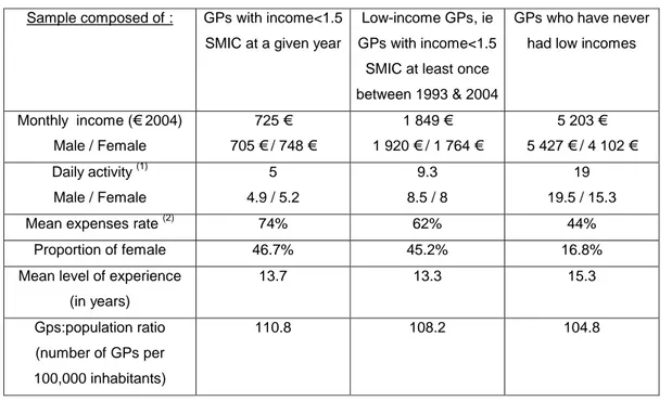
Basic features of the data are displayed in table 2. If we suppose that GPs work about

2_{Reliable data on the earnings of self-employed workers in general are rare. French ambulatory care}

administration produces reliable data on physicians’ earnings : the public health insurance scheme observes GPs’earnings because it reimburses patients for their payments to doctors.

3_{Depending on the GP’s location and level of activity, these expenses represent between 35% and}

300 days a year4_{, they see about 19 patients per day which ensures them a monthly} income of about 5,000e (third column). Female GPs work less than their male counter-parts: they only see around 15 patients per day. Indeed, descriptive studies have shown that they work less hours per day, less days per week and their visit duration is longer (Fivaz and Le Laidier, 2001). GPs who have low incomes at a given year (ie income lower than 1.5 net SMIC) only have about 5 patients a day, for a monthly income of 800 e (…rst column). While female GPs represent only 17% of all practicing GPs between 1993 and 2004, they are over-represented among those GPs with low incomes. One can see no signi…cant di¤erence in the average experience level of low-income GPs and other GPs. The second column displays average …gures calculated over the whole career of GPs who experienced low-income at least once between 1993 and 2004, ie on GPs who compose our sample of "low-income GPs". As they earn on avearge 1,850e a month, their incomes are not lower than 1.5 SMIC over their whole career. But they have a much lower activity than all GPs. Section 3 characterizes more precisely who are these "low-income GPs".

Table 2: Basic features of the data

Sample composed of : GPs with income<1.5 SMIC at a given year

Low-income GPs, ie GPs with income<1.5

SMIC at least once between 1993 & 2004

GPs who have never had low incomes

Monthly income (€ 2004) Male / Female 725 € 705 € / 748 € 1 849 € 1 920 € / 1 764 € 5 203 € 5 427 € / 4 102 € Daily activity(1) Male / Female 5 4.9 / 5.2 9.3 8.5 / 8 19 19.5 / 15.3

Mean expenses rate(2) 74% 62% 44%

Proportion of female 46.7% 45.2% 16.8%

Mean level of experience (in years) 13.7 13.3 15.3 Gps:population ratio (number of GPs per 100,000 inhabitants) 110.8 108.2 104.8 Notes :

(1) Activity is composed of o¢ ce visits, home visits, surgery and radiology acts; (2) The expenses rate is the proportion of charges (rent for the o¢ ce, payments of the secretary, etc.) in GP’s total earnings. The amount of charges is then deducted from earnings to compute earnings net of expenses, ie what we call in this paper GPs’net income.

3

Is there a kind of low-income GPs?

Considering the sample of GPs who experienced a period of low incomes at least once between 1993 and 2004, one can observe that the period during which GPs have low incomes lasts on average 5.7 years.5 _{But for more than 50% of them, this period lasts} less than 2 years. This situation seems to be transitory.

However, …gure 1 shows that having low incomes even during a short period of time has a lasting impact on GPs’ incomes over their whole career. For example, 5 years after the …rst year of low incomes, 30% of GPs have quitted the self-employed GP profession (probably for becoming salaried doctors6_{) and for 55% of GPs, incomes remain below}

5_{GPs are observed during a maximum period of 12 years in the panel.} 6_{The reasons why GPs leave the sample are not observed.}

the …rst two deciles of the distribution of incomes of all GPs. Mobility is rare: only 15% of GPs experience a small rise in their income, but their income do not exceed the …rst quartile of the distribution of income of all GPs. Despite these lasting low incomes, one can …nd surprising that the vast majority of low-income GPs chooses to remain self-employed.

Figure 1: Mobility in incomes after the …rst year of low-incomes

0 10 20 30 40 50 60 70 80 90 100 t+1 t+2 t+3 t+4 t+5 t+6 t+7 t+8 t+9 t+10 t+11 Number of years after the first year of low incomes

In %

Exit D1-D2 D3-D6 D7 and +

To understand if low-income GPs have di¤erent characteristics than all other GPs, we use the sample composed of all GPs and run a probit model where the dependent variable Yit equals 1 if the GP has low incomes (incomes lower than 1.5 SMIC) at a given year t. This binary variable is determined by the sign of an unobserved latent variable Yit, whose expectation is a linear combinaison of the characteristics of GP i at

year t: The speci…cation is the following: Y_it = X_it0 + uit (1) Yit = 8 < : 1 if Y_it 0 0 if Y_it < 0

Vector Xit0 comprises the following (qualitative) variables :

Dummies relative to the geographic location of GPs: région of practice, type of location (rural area, small town, big town, city), the number of GPs per 100,000 inhabitants and the number of specialists per 100,000 inhabitants in the départe-ment where GP i works.

Dummies relative to the GP and his activity: experience, gender and time dum-mies.

Dummies caracterizing the beginning of practice of the GP: the lenght between year of PhD and …rst year of practice, the age he obtained his PhD, dummies relative to the year of beginning of practice.

This model is estimated using two di¤erent methods: i) a pooled probit model; ii) a probit random e¤ects model. Model i) does not take into account that the error term is likely to be correlated over time for a given GP : uit ! N(0; 1). Model ii) allows us to capture unobserved individual heterogeneity. We suppose that uit = i + "it, where i is an individual speci…c unobservable e¤ect that is supposed to be distributed independently of the regressors. We have:

0 @ i "it 1 A N 0 @ 0 @ 0 0 1 A ; 0 @ 2 0 0 1 1 A 1 A The composite error is equicorrelated :

corr(uit; uis) = = 2 2 ₊ 2

"

In order to deal with the potential correlation of the individual speci…c e¤ect with the regressors, one could alternatively estimate a …xed e¤ects logit model. Such estimation is impossible given the structure of our sample. GPs whose status remains constant over time (low incomes or not) do not contribute to the likelihood so that only 9% of our observations could be used. The sample would be too small to carry out a robust econometric analysis. In our model, potential endogeneous variables are mainly variables relative to the location of GPs, such as the physician:population ratio, the regional …xed e¤ects and the type of location. Indeed, Bolduc et al. (1996) have shown that doctor’s location choices are in‡uenced by expected earnings in each location. If i is correlated to the region of pratice for example, coe¢ cients related to this variable will re‡ect the in‡uence of the region of practice on the probability of having low incomes, biaised by the the in‡uence of the unobserved individual e¤ects. However, given the small number of available instruments, we cannot resolve this endogeneity problem7_.

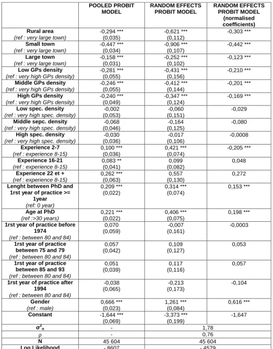
Results of the estimation of model (1) are presented in table 3. Table 4 presents the estimations carried out separately on male and female GPs.

The estimation of the probit random e¤ects model shows that the individual speci…c e¤ect explains 76% of the total variation of the disturbance (75% for male and 81% for female GPs). The proportion of behaviours not explained by the model is therefore due to di¤erences between GPs more than accidental reasons. This result con…rms the persistence of low-incomes: compared to inter-individual di¤erences, there is a large temporal inertia.

7_{We are limited by the small number of available instruments to check and correct for the potential}

endogeneity of variables linked to the location of doctors. However, we were able to check for exogeneity of the GP:population ratio, following Rivers and Vuong procedure (1988) described by Wooldridge (2002) : i) In a …rst step, we regress the density variables on the exogenous variables of the model and the excluded instruments. We used as instruments variables explaining demand for care services in each département : the proportion of women, the proportion of inhabitants aged 60 and more as well as the logarithm of average household income in the département. The specialists:population ratio, which is not signi…cant in the regression, was also added to the list of instruments; ii) in the second step, we re-estimate model (1) including residuals obtained from the …rst step. The test of joint signi…cance of the estimated residuals lead to non-rejection of the asumption that the GP:population ratio is exogeneous (p=0.531). However, our tests are limited by the small number of instruments. We were not able to carry out an exogeneity test for regional dummies, which are also related to location choice.

There is not much di¤erences between the pooled probit and the random e¤ects models8_. Discrepancies (between experience, density or regional e¤ects) seem lower when using the random e¤ects speci…cation, probably because the model is better speci…ed. We only comment results obtained from the pooled probit model, as predicited probabilities are easier to compute with this model. We measure how the probability of having low incomes for a reference GP changes when we change his characteristics. The reference GP is a men, living in Paris, praticing in 1993, who has between 8 and 15 years of experience and who began his career in the 1980s. He obtained his PhD thesis at the age of 30 and started praticing immediately after. He has a 5% chance of having low incomes.

The …rst striking result is the very small impact of experience on the probability of having low incomes. The probability of having low-incomes is 6.1% at the beginning of the career (less than 7 years of experience), 5.9% between 16 and 21 years of experience and 8.4% after 22 years. Di¤erences in these probabilities are small9_{. We would expect} low income GPs to be GPs beginning their career, experiencing di¢ culties in the process of patient recruitment. This is not the case.

Secondly, while female GPs represent only 1/5 of GPs practicing between 1993 and 2004, the probability of experiencing low incomes rises from 5% for a man to 16.4% for a woman. Moreover, while the probability of having low incomes decreases to 2.6% for a man practicing in rural areas, women are as likely to have low incomes in rural as in urban areas (16.4%). These results bring several interpretations. Do they mean that some female doctors su¤er discrimination from some kinds of patients? (for example, old patients or patients living in rural areas who are less used to see a female doctor). Or do they mean that some female GPs have a preference for leisure leading to a lower number of hours of work and a higher probability of having low-incomes? Unfortunately,

8_{Coe¢ cients associated to the random e¤ects probit model are normalised and are therefore}

com-parable to those obtained from the pooled probit model.

9_{Estimates of the random e¤ect probit model even show that the probability of having low incomes}

our database does not provide any information on doctors’ household composition or hours of work. These informations would enable us to go further in exploring the two possible explanations. Separate regressions on male and female (table 4) however show that, contrary to men, very few observable variables explain the probability for a woman to have low incomes, which could con…rm the preference hypothesis.

Thirdly, variables related to the geographic location of GPs have a strong impact on the probability of having low incomes. This probability decreases from 5% to 2.7% when the reference GP practices in a small densely populated area instead of in Paris (an area where the density is high). As the GP:population ratio provides a measure of the competition intensity between physicians within each département, this result is intuitive: it is easier for a GP to recruit patients in areas where there is less competition. Surprisingly, the specialists:population ratio is non signi…cant. GPs do not seem to compete with specialists.

The in‡uence of GP density comes on top of regional …xed e¤ects. These regional …xed e¤ects capture the time-invariant impact of certain characteristics of regions on the probability of having low incomes : amenities, average GPs:population ratio and determinants of demand for care services. Estimates of these regional …xed e¤ects are presented on …gure 2. The probability of having low-incomes is much stronger for a GP who practices in the south of France than in the Paris area (the reference category). Conversely, this probability is signi…cantly smaller in the north of France. On the demand side, these di¤erences come from the fact that more GPs share a given number of potential patients in the souh of France, where medical density is high, increasing the probability of having low incomes. But medical density is still high in the north of France and yet the probability of having low incomes is rather small. Another interpretation than competition between GPs therefore explains the discrepancies between regions : the importance given to the quality of life. At the end of their studies, medical students can freely choose the area where they want to practice. 75% of them choose to locate in areas close to the medical school they attended. This

is not speci…c to french doctors, as shown by Eisenberg and Cantwell (1976) for the United States. Most of the remaining 25% choose to locate in the sunniest regions of France, where quality of life is reputed to be better, i.e. in the South or South-West of France10_{. Two di¤erent interpretations can therefore explain the over representation} of low income GPs in the south of France : i) more intense competition increases the probability of having low incomes; ii) GPs who want to work less settle in regions where the quality of life is better (when leisure is important, quality of life matters more). All these results lead to one important question: are low-income GPs constrained by a lower demand (discrimination from some patients, high level of medical density) or do they choose to work less and have a preference for leisure? In other words, do they have a di¤erent optimal level of activity than all other GPs?

Table 3: Estimation of the probability of having low incomes. Results of the pooled probit model (column 1) and the random-e¤ects probit model (columns 2 and 3)

POOLED PROBIT MODEL RANDOM EFFECTS PROBIT MODEL RANDOM EFFECTS PROBIT MODEL (normalised coefficients) Rural area

(ref : very large town)

-0,294 *** (0,035) -0,621 *** (0,112) -0,303 *** Small town

(ref : very large town)

-0,447 *** (0,034) -0,906 *** (0,107) -0,442 *** Large town

(ref : very large town)

-0,158 *** (0,031) -0,252 *** (0,102) -0,123 *** Low GPs density

(ref : very high GPs density)

-0,281 *** (0,055) -0,431 *** (0,156) -0,210 *** Middle GPs density

(ref : very high GPs density)

-0,246 *** (0,055) -0,412 *** (0,144) -0,201 *** High GPs density

(ref : very high GPs density)

-0,240 *** (0,049)

-0,347 *** (0,124)

-0,169 ***

Low spec. density

(ref : very high spec. density)

-0,002 (0,053)

-0,060 (0,151)

-0,029

Middle sepc. density

(ref : very high spec. density)

-0,068 (0,046)

-0,164 (0,125)

-0,080

High spec. density

(ref : very high spec. density)

-0,030 (0,036) -0,017 (0,106) -0,0008 Experience 2-7 (ref : experience 8-15) 0,100 *** (0,036) 0,421 *** (0,074) -0,205 *** Experience 16-21 (ref : experience 8-15) 0,083 ** (0,041) 0,099 (0,082) 0,048 Experience 22 et + (ref : experience 8-15) 0,262 *** (0,063) 0,557 (0,130) 0,272

Lenght between PhD and 1rst year of practice >= 1year (ref: 0 year) 0,209 *** (0,022) 0,314 *** (0,074) 0,153 *** Age at PhD (ref :>30 years) 0,221 *** (0,022) 0,406 *** (0,075) 0,198 ***

1rst year of practice before 1974

(ref : between 80 and 84)

0,070 (0,059) -0,007 (0,161) -0,0003 1rst year of practice between 75 and 79

(ref : between 80 and 84)

0,057 (0,042) 0,109 (0,127) 0,053 1rst year of practice between 85 and 93

(ref : between 80 and 84)

0,051 (0,039)

0,117 (0,116)

0,057

1rst year of practice after 1994

(ref : between 80 and 84)

-0,038 (0,065) -0,213 (0,173) -0,104 Gender (ref : male) 0,666 *** (0,023) 1,261 *** (0,084) 0,616 *** Constant -1,644 *** (0,069) -3,373 *** (0,199) -1,647 σ2 α - 1,78 ρ - 0,76 N 45 604 45 604 Log Likelihood - 8607 - 4579 Notes :

*** coe¢ cients are statistically signi…cant at the 1% level; ** statistically signi…cant at the 5% level; * statistically signi…cant at the 10% level; Standard errors are reported in parentheses. In the third column, coe¢ cients of the random e¤ects probit model are normalised to be comparable to those obtained from the pooled probit model : they are divided byp(1 + 2_).

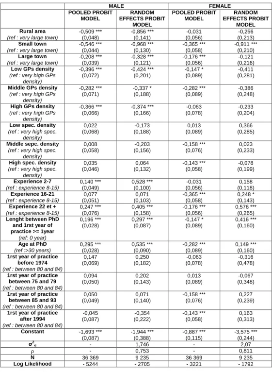
Table 4: Estimation of the probability of having low incomes, separately for male and female. Results of the pooled probit model (columns 1 and 3) and the random-e¤ects probit model (columns 3 and 4)

MALE FEMALE POOLED PROBIT MODEL RANDOM EFFECTS PROBIT MODEL POOLED PROBIT MODEL RANDOM EFFECTS PROBIT MODEL Rural area

(ref : very large town)

-0,509 *** (0,048) -0,856 *** (0,141) -0,031 (0,056) -0,256 (0,213) Small town

(ref : very large town)

-0,546 *** (0,044) -0,968 *** (0,130) -0,365 *** (0,058) -0,911 *** (0,210) Large town

(ref : very large town)

-0,208 *** (0,039) -0,328 *** (0,121) -0,176 *** (0,056) -0,121 (0,216) Low GPs density

(ref : very high GPs density) -0,396 *** (0,072) -0,424 *** (0,201) -0,147 * (0,089) -0,411 (0,281) Middle GPs density

(ref : very high GPs density) -0,282 *** (0,071) -0,337 * (0,188) -0,282 *** (0,089) -0,386 (0,248) High GPs density

(ref : very high GPs density) -0,366 *** (0,066) -0,374 *** (0,166) -0,063 (0,078) -0,233 (0,204)

Low spec. density

(ref : very high spec. density) 0,022 (0,068) -0,173 (0,188) 0,013 (0,089) 0,366 (0,285)

Middle sepc. density

(ref : very high spec. density) 0,008 (0,058) -0,203 (0,156) -0,158 *** (0,076) 0,023 (0,233)

High spec. density

(ref : very high spec. density) 0,035 (0,046) 0,064 (0,132) -0,143 *** (0,058) -0,078 (0,199) Experience 2-7 (ref : experience 8-15) 0,140 *** (0,049) 0,528 *** (0,100) -0,031 (0,056) 0,158 (0,118) Experience 16-21 (ref : experience 8-15) 0,077 (0,051) 0,071 (0,103) -0,365 *** (0,058) 0,248 * (0,143) Experience 22 et + (ref : experience 8-15) 0,247 *** (0,076) 0,405 *** (0,158) -0,176 *** (0,056) 0,576 *** (0,265) Lenght between PhD and 1rst year of practice >= 1year (ref: 0 year) 0,196 *** (0,028) 0,297 *** (0,087) -0,147 * (0,089) 0,416 *** (0,160) Age at PhD (ref :>30 years) 0,295 *** (0,028) 0,535 *** (0,090) -0,282 *** (0,089) 0,149 *** (0,160) 1rst year of practice before 1974

(ref : between 80 and 84)

0,147 (0,069) 0,250 (0,182) -0,063 (0,078) -0,316 (0,478) 1rst year of practice between 75 and 79

(ref : between 80 and 84)

0,094 (0,050) 0,202 (0,143) 0,013 (0,089) -0,067 (0,348) 1rst year of practice between 85 and 93

(ref : between 80 and 84)

0,050 (0,049) 0,071 (0,140) -0,158 *** (0,076) 0,227 (0,239) 1rst year of practice after 1994

(ref : between 80 and 84)

-0,045 (0,087) -0,354 (0,222) -0,143 *** (0,058) 0,163 (0,313) Constant -1,693 *** (0,087) -1,944 *** (0,388) -0,887 *** (0,115) -3,575 *** (0,244) σ2 α - 1,746 - 2,07 ρ - 0,753 - 0,811 N 36 369 9 235 36 369 9 235 Log Likelihood - 5244 - 2705 - 3221 - 1792 Notes :

*** coe¢ cients are statistically signi…cant at the 1% level; ** statistically signi…cant at the 5% level; * statistically signi…cant at the 10% level; Standard errors are reported in parentheses.

Figure 2: Geographic location of low income GPs in France - Results obtained from the pooled probit model.

4

Do low-income GPs choose to work less?

4.1

Theoretical framework

As fees are …xed, we adopt a …xed price equilibrium approach. We use a model built by Bolduc et al (1996) to study doctors’ location choices and we suppose that GPs maximize their utility U (l; c; x) to set their level of activity. l represents hours in leisure activity, c the level of consumption and x individual attributes that can be observed or not. Utility is assumed to be quasi-concave.

Results from the previous section lead us to test whether low income GPs have di¤erent preferences than all other GPs. We suppose that there are two kinds of utility functions :

where j = 1 for a GP i who does not have low incomes and j = 2 for a low-income GP i.

Keep in mind that low-income GPs are GPs who have had, at least once between 1993 and 2004, incomes lower than 1.5 times the French minimum wage.

Each physician is supposed to maximize his utility to de…ne his optimal level of activity, denoted A_i, subject to a double constraint : the production function and the demand function he faces.

The budget constraint for GP i of type j is :

pc cij = p Aij; i = 1::::N and j = 1; 2: (3)

where Aij is the level of activity of GP i of type j (mostly home and o¢ ce visits). Aij = T lij where T is the total …xed amount of time that can be allocated between labour and leisure.

pis the price for an encounter, the reference fee, …xed by agreement between physicians and the health insurance administration. This price is therefore exogeneous and it is the same for all GPs belonging to sector 1.

As fees are …xed, fee levels have no in‡uence on demand for services from a particular physician. The demand faced by each GP depend on the population health status, measured at the département level (hd), the number of GPs operating in the same area (the potential level of demand faced by the physician), denoted dd and a GP speci…c variable vij11. Demand is therefore de…ned as:

d_ij;(i2d) = Dd+ ij where Dd = f (hd; dd)

The variable vij allows us to introduce heterogeneity in the demand faced by GPs

11_{The demand faced by a GP could also depend on the number of specialists. But a previous study}

(Dormont and Samson, 2008) has shown that the specialists:population ratio does not a¤ect GPs’level of activity.

within each département. It represents the market share of the GP, linked to his ability to recruit and keep patients. It can also measure potential discrimination towards some GPs, for example female GPs.

Because prices are …xed in sector 1, the price of an encounter cannot be used to adjust the supply and the demand faced by the GP (as it would be the case if we had adopted a market for ambulatory care characterized by a monopolistically competitive structure, as in McGuire (2000)). Therefore :

Aij dij (4)

Moreover, we do not suppose that the equilibrium is obtained by adjustments in care quality. Indeed, this would imply that the minimum level of care quality provided during an encounter can be very low, which seems unrealistic. It would also mean that care quality provided by a low-income GP is rather low, which is not proved.

In this speci…cation, low income GPs only di¤er from the other GPs by their preferences in the labour-leisure trade-o¤. The optimal level of activity of GP i of type j, denoted A_ij(p)is obtained by maximising the utility function (2) under constraints (3) and (4).

4.2

A microeconometric test of low-income GPs’ preference

for leisure

To test if low-income GPs choose to work less than all other GPs or if they are con-strained to, we measure their reaction to a shock of demand.

Let consider a low income GP i (i 2 j = 2);whose optimal level of activity is denoted A_i. He faces the demand di = Dd + i: Theoretically, a shock of demand di can in‡uence his level of activity in two di¤erent ways :

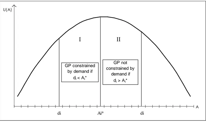
If low-income GPs are constrained to work less than all other GPs, their optimal level of activity A_i is higher than the demand di that they face. Constraint (4) is saturated. Their e¤ective level of activity is Ai = di < Ai. They are located in

the area I of …gure 3. A positive shock of demand di > 0 will lead to an increase in their activity : it allows them to move closer to their optimal level of activity. A negative shock of demand di < 0 will lead to a decrease in their activity:

8 < :

di > 0) Ai > 0 di < 0) Ai < 0

Let us denote + the elasticity of GP’s activity with respect to a positive shock of demand and the elasticity of GP’s activity with respect to a negative shock of demand. If low-income GPs have a low level of activity because they are constrained by the demand they face, we have:

+ _{> 0 and > 0}

If low-income GPs choose to work less hours than all other GPs, they are not constrained by the demand: their optimal level of activity is lower that the de-mand they face. Their e¤ective level of activity is Ai = Ai di. They are located in the area II of …gure 3. These GPs refuse patients. A positive shock of demand di > 0 will have no in‡uence on their activity as they have already reached their optimal level of activity. Respond to the increasing demand by increasing their activity would reduce their utility. A negative shock of demand di < 0 will lead to a decrease in their activity (if the variation of demand is such as they move from area II to area I on …gure 3), or will have no in‡uence on their activity (if we stay in area II) :

8 < :

di > 0) Ai > 0 di < 0) Ai < 0

If low-income GPs have a preference for leisure and choose to work less hours than all other GPs, we have:

+

To sum up, a su¢ cient condition to discriminate between the two intial hypotheses and to conclude that low-income GPs choose to have a lower level of activity than all other GPs is to test their reaction to a positive shock of demand. The econometric speci…cation presented in this section consists therefore of testing the null hypothesis12 :

H0 : += 0

Figure 3: Representation of a Utililty function U (A) for a low-income GP, given his level of activity A di Ai* di U(A) A GP constrained by demand if di< Ai* GP not constrained by demand if di > Ai*

I

II

12_{Given this speci…cation, we can also characterize the behaviour of all other GPs, the only di¤erence}

being that they have a higher optimal level of activity than low-income GPs. They can be, or not, constrained by the demand they face. Results from the econometric speci…cation will also enable us to discriminate between these two hypotheses.

4.3

Empirical speci…cation

Consider actidt the log of activity of physician i practicing in year t in the département d. Our speci…cation is the following :

actidt = + demdt+ Xit0 + t+ d+ i+ "idt (5) with i = 1; :::N ; t = 1; :::T ; d = 1; :::D

Vector X0

itincludes variables relative to GP i (such as experience, gender,...), tare year-speci…c dummies, dare département …xed e¤ects and iare individual unobserved …xed e¤ects. They include GPs’ability to attract and keep patients but also GPs’preference for leisure in the labour-leisure trade-o¤. demdt is the log of demand faced by the physician i in his département d at year t: This demand includes the two variables previously de…ned :

demidt = log

health expendituresdt medical densitydt

Health expenditures are the total amount of health expenditures spent by the inhab-itants of département d at year t (de…ned in 2004 euros and for 100,000 inhabinhab-itants). It includes pharmaceutical expenditures as well as the amount spent for encounters to GPs or specialists13_{. Medical density is the number of GPs per 100,000 inhabitants in} a département d at year t.

First-di¤erencing this equation enables us to carry out our test which is founded on the reaction of GPs to a positive shock of demand. Written in …rst-di¤erences, speci…cation (5) becomes : : actidt = : demdt+ t+ : "it (6)

Variablesact:idt and :

demdt are the …rst di¤erences of the logarithms (i.e. the growth

13_{The annual series of these variables are available in the data base Eco-Santé (2008), available}

rates) of activity and demand of GP i at year t in the département d: measures the elasticity of the GPs’activity with respect to a shock of demand. This speci…cation is inspired by Delattre and Dormont (2003) who test the existence of physician-induced demand by measuring the reaction of GPs (in terms of number of encounters and of volume of care delivered in each encounter) to a variation in the phyisician:population ratio. This speci…cation leads to eliminate the individual and departement unobserved …xed e¤ects d and i as well as variables relative to GP i which are mainly constant over time14_.

The shock of demand :

demdtcombines the e¤ects of a positive and a negative shock of demand, that we need to distinguish in order to carry out our test. Our …nal speci…cation is the following: : actidt = + : dem>0_dt + : dem<0_dt + t+ : "idt (7) +

is the elasticity of GP’s activity with respect to a positive shock of demand (denoted

: dem>0

dt ) and is the elasticity of GP’s activity with respect to a negative shock of demand (denoted

: dem<0_dt ).

To test the reaction of low-income GPs to a shock of demand and to compare their reaction to that of all other GPs, model (7) is estimated separately on low-income GPs (i.e. GPs who have had, at least once between 1993 and 2004, incomes lower than 1.5 SMIC) and all other GPs.

Model (7) is also estimated on GPs who have more than 7 years of experience. We know (Dormont and Samson, 2008) that earnings are a U-shaped function of experience, characterized by a huge increase in earnings at the beginning of the practice (during the …rst seven years) and a rapid decrease after 12 years of practice. This restiction is necessary to avoid coe¢ cients to be in‡uenced by this rapid growth in activity at the beginning of the career15_.

14_{This is not the case for the experience variable, but this variable increases by 1 every year.} 15_{However, our results remain unchanged when estimation are performed on all GPs, whatever their}

The demand variable is not exogenous, as it includes encounters delivered by GPs. Therefore, estimation of model (7) in …rst-di¤erences using ordinary least squares (OLS) gives non consistent estimates. Model (7) is therefore also estimated in …rst-di¤erences using instrumental variables (IV) but also by the generalized method of moments (GMM).

16 instruments are used to instrument the positive and negative shocks of demand for the estimation by IV. We have at our disposal the number of cases of ‡u and of gastro-enteritis by région over the years 1993-2004 (Réseau Sentinelles, INSERM, 2008). These variables are not signi…cant when they are used as explanatory variables in model (7) but they are good explanatory variables of demand for health care and therefore good potential instruments. We use the log of these variables in t, t 1 and t 2. We also use as instruments the log of the proportion of inhabitants aged 60 or more, the log of average household income and the log of the GPs:population ratio. These three variables are de…ned at the département level and are used in t, t 1and t 2:We also include the log of activity of GP i in t 2. These instruments must be exogeneous (Sargan test), su¢ ciently correlated to

: dem>0

dt and : dem<0

dt (not weak instruments) and must be unsigni…cant in model (7). The exogeneity of variables

:

dem>0_dt and :

dem<0_dt is tested using the Hausman test. Results of these tests are presented in the appendix.

Model (7) is also estimated by GMM, as presented by Arellano and Bond (1991) for panel data sets. This method enables us to get consistent and e¢ cient estimates, as long as instrument validity is con…rmed by the Sargan test. This method usually uses lagged observations of endogeneous variables as instruments. But these instruments were not validated by the Sargan test. We therefore use as instruments the lags zit sof the instruments used for the IV estimation. We use lags s 0 for all variables, except the log of GPs’ activity (s 2). Standard errors are corrected using Windmeijer’s correction (2005).

Both methods provide consistent estimations, but if the Sargan test validates the ex-ogeneity of instruments, the GMM estimation is more e¢ cient as it uses more

ments16 _{and a more important part of the available information by taking the structure} of the covariance matrix of the disturbance into account.

4.4

Results

4.4.1 Main results

Estimates of model (7) are presented in table 5. Columns 1 to 3 concern GPs who have never had low incomes during their career (observed between 1993 and 2004) and columns 4 to 6 concern low-income GPs.

Concerning GPs without low incomes, the OLS estimates (column 1) show that a positive shock of demand has a positive impact on the level of their activity ( + = 0; 366) and that a negative shock of demand reduces their activity ( = 0; 403). These two reactions are not signi…cantly di¤erent. As these results are not consistent, the model is also estimated by IV:

: dem>0

dt et dem <0

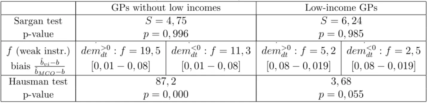
dt ;that are not exogenous are instrumented using the 16 instruments previously described. The value of + is close to the one obtained using OLS ( + = 0; 303) but GPs react more heavily to a negative shock of demand ( = 1; 101). Moreover, standard errors are four times higher than in column 117_{. But coe¢ cients are still signi…cant. The hypothesis of instruments exogeneity is} validated by the Sargan test (table A in the apendix) (p = 0; 99): Moreover, instruments are su¢ ciently correlated to the explanatory variables. The Fisher statistics is 19.5 when instrumenting

:

dem>0_dt and 11.3 for :

dem<0_dt . In accordance with Bound, Jaeger et Baker (1995), the biais induced by the use of instrumental variables is comprised between 1 and 8% of the biais linked to the use of OLS. Instruments are not weak instruments. The Hausman test rejects exogeneity of variabes

: dem>0

dt and dem <0

dt (p = 0; 000).

16_{To improve the e¢ ciency of the instrumental variable estimator, we could add more instruments}

or more lags to the instruments used. This last solution would however reduce the size of our sample.

17_{This small e¢ ciency is due to the loss of variability induced by the projection of} :

dem<0_dt and

:

dem>0

dt on the instruments. The R2obtained in the …rst-step regression shows that we lose 80% of the

variability of

:

dem<0_dt(only 15% for

:

dem>0_dt): To improve e¢ ciency, one should use more instruments, that we do not have.

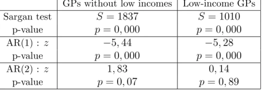
Estimations provided by GMM lead to comparable estimates ( + = 0; 285 et = 0; 768). The test of non autocorrelation at order 2 of ":dt is validated: this justi…es the use of the lags t s of the log of GPs’ activity from s 2 (as E(actit 2;

:

"dt) = 0). But the Sargan test does not validate exogeneity of the instruments (table B in the appendix)18_.

Low income GPs never react to a positive shock of demand, while it would give them the opportunity to increase their activity and their incomes. Whatever estimation is considered, we …nd that + = 0: They only react to a negative shock of demand: they reduce their activity when they are constrained to (because of a decrease in demand for health care or an increse in the GPs:population ratio). Their reaction to a negative shock of demand is non signi…cantly di¤erent from the one obtained for all other GPs. Therefore, the two kinds of GPs only di¤er by their reaction to a positive shock of demand. Our …nding that low-income GPs never react to a positive shock of demand suggests that they have already reached their optimal level of activity. Our hypothesis seems to be validated : low-income GPs work less than all other GPs because they choose to have a low level of activity. The cost of e¤ort needed to increase their activity when demand is increasing is too high. They have a strong preference for leisure. However, this result is more a clue than a proof that low-income GPs choose to work less. Indeed, the Sargan test does not validate the exogeneity of the instruments in the estimation by GMM. Moreover, coe¢ cients obtained with the IV estimation can be biaised: although the instruments are exogenous, the Fisher statistic (5.2 when instrumenting : dem>0 dt and 2.5 for : dem<0

dt ;table A in the appendix) shows that they are probably weak instruments. The biais induced by the use of IV is comprised between 8 and 19% of the biais associated to the use of OLS.

Note that our results are maintained when model (7) is estimated separately on male and female physicians.

18_{Reducing the number of lags included in the estimations (by taking, for example, s 6) reduces}

the Sargan value, but the Sargan test still leads to reject instrument validity. Values taken by +and are not much a¤ected by the number of lags used.

Table 5: Estimates of model (7) in …rst-di¤erences by OLS (columns 1 and 4), in …rst-di¤erences by IV method (columns 2 and 5) and by GMM (columns 3 and 6).

GPs without low incomes Low-income GPs OLS IV GMM OLS IV GMM : dem>0_it 0.366 *** 0.303 *** 0.285 *** -0.022 -0.269 -0.077 (0.041) (0.181) (0.057) (0.217) (0.649) (0.426) : dem<0_it 0.403 *** 1.101 *** 0.768 *** 0.455 * 1.178 *** 0.757 ** (0.144) (0.664) (0.215) (0.271) (0.527) (0.395) Notes :

(i) Estimation on sector 1 GPs, who have more than seven years of experience. Estimation period: 1993-2004;

(ii) All estimations include time dummies (t95:::t04)that are signi…cant at the 5% level;

(iii) Standard errors are reported in parentheses. For the estimation by OLS and by IV, we use cluster-robust standard errors that cluster on the individual (and therefore control for the correlation over time of the error term, for a given individual). For the estimation by GMM, they are two-step estimates of standard errors, corrected by Windmeijer’s correction (2005) ; (iv) *** coe¢ cients are statistically signi…cant at the 1% level; ** statistically signi…cant at the 5% level; * statistically signi…cant at the 10% level;

(v) Estimation by GMM is performed using the STATA "xtbond2" command (Roodman, 2006) ;

(vi) Both variables

:

dem>0_it and

:

dem<0_it are instrumented. 16 instruments are used for the esti-mation by IV: lags int; t 1ett 2of the log of cases of ‡u, log of cases of gastro-enteritis, log of the proportion of inhabitants aged 60 or more, log of average household income and log of the GPs:population ratio, as well as lag int 2 of the log of GPs’activity.

(vii) Estimation by GMM uses lags int s of these instruments, with s 2 for the log of activity ands 0 for the other variables -Total number of instruments: 438 ;

(viii) For the estimation in …rst-di¤erences by IV, results of the Hausman test, weak instru-ments and Sargan test are presented in table A of the appendix. For the estimation by GMM, results of the Sargan tests and tests of autocorrelation of ":dt at order 1 and 2 are presented

in table B of the appendix.

4.4.2 Robustness check : selection biais

The estimates of model (7) for low-income GPs may be a¤ected by a selection biais. Figure 1 shows that …ve years after the …rst year of low incomes, 30% of GPs have quitted the self-employed GP profession, probably to increase their level of income. This proportion di¤ers greatly between male and female doctors : 33% of male GPs made this choice against only 17% of low-income female GPs. The reasons why doctors leave the

sample are not observed, but most of them probably become salaried doctors or doctors working in schools or within …rms. One can think that GPs who choose to remain self-employed, despite their low incomes, are GPs who are satis…ed with their level of income. Consequently, our estimates can be biaised. Unobservables characteristics of low-income GPs who choose to remain self-employed (their preference for leisure for example) can in‡uence their response to the di¤erent shocks of demand.

To check for the existence of an attrition biais and correct it, if necessary, we use the procedure described in Wooldridge (2002), based on the Heckman’s sample selection model. The participation equation estimates the probability for a low-income GP to remain self-employed …ve years after his …rst year of low incomes. We use the following explanatory variables : gender, région of practice, GPs:population ratio in the départe-ment of the GP, the level of experience when the GP …rst experienced low incomes, the age he got his PhD and the number of years between year of PhD and …rst year of practice. We want to approximate the probability for the GP to be satis…ed with the relatively low level of his incomes. The second step is the estimation of model (7) on low-income GPs who remain self-employed at least 5 years after their …rst year of low incomes. The inverse of the mills ratio is introduced as an additional explanatory variable. The model is also estimated separately on male and female.

Estimates of the participation equation19 _{show that the probability of remaining} self-employed despite low incomes is higher for women than men, for GPs who …rst expe-rience low incomes in the …rst …ve years of their career, for GPs who work in rural areas and for GPs who delay their beginning of career after the obtention of their PhD. The Mills ratio included in model (7) is not signi…cant (t = 0:62), which validates the estimates presented in table 5.

When we distinguish women from men, one …nds that the mill ratio is still not signif-icant for men (t = 0:77) but becomes signi…cant for women (t = 3:04). Coe¢ cients of model (7) for low-income female GPs are therefore potentially biaised. However, estimates of model (7) on women who choose to remain self-employed, with or without

the introduction of the mills ratio , always lead to the same conclusion. We …nd that + _{= 0; which con…rms the preference for a low level of activity and therefore low} incomes.

5

Discussion and conclusion

In this paper, we use a longitudinal data set that covers more than 4,000 French self-employed GPs observed over the 1993-2004 period. We …nd high disparities in French GPs’incomes : each year between 1993 and 2004, 5 to 7% of GPs earn less than 1.5 times the level of the French minimum wage. The purpose of this paper is to study those "low-income GPs", i.e. GPs who have had, at least once between 1993 and 2004, incomes lower than this limit. The descriptive analysis shows four main patterns : i) For these low-income GPs, experiencing low incomes, even during a short period of time, has a lasting impact on their incomes over their whole career; ii) Surprisingly, low-income GPs are not young physicians who begin their activity and who have di¢ culties in recruiting patients; iii) low-income GPs are mainly female doctors; iv) but also physicians practicing in the south of France, i.e. in areas where the medical density is very high but where the quality of life is also better. As self-employed workers, French GPs are free to choose the number of hours they want to work. These …ndings therefore lead to one question : do low-income GPs choose to work less than all other GPs or are they constrained to? In other words, do they have more preference for leisure than the other french self-employed GPs? The econometric analysis consists of measuring GPs’ reaction to an exogeneous shock of demand. It shows that low-income GPs never react to an increase in demand, while it would give them the opportunity to increase their activity and their incomes. They only react to negative shocks of demand, i.e. they decrease their activity when they are constrained to. Conversely, all other GPs always react to positive and negative shocks of demand : their activity is strongly constrained by the demand they are facing. We conclude that those low-income GPs are physicians who choose to work less : to respond to the increasing demand by increasing their

activity would reduce their utility. Their low incomes do not re‡ect a downgrading of the GPs’profession, but rather one of its advantages: as self-employed, GPs can freely choose their number of hours of work. They may choose to work less.

This result is consistent with two observations in our data set :

Some low-income GPs quits the self-employed GP profession prematurely, but not all. Those who remain self-employed may be GPs who are satis…ed with their level of income.

Experiencing low incomes is strongly linked to the geographic location of the physician. To increase their activity and their incomes, GPs could move to another location where the level of the GPs:population ratio is lower (a rural area for example). But none of the low-income GPs belonging to our sample makes this decision.

These results show that the behaviour of low-income GPs could be motivated by the existence of a target-income. Those GPs refuse patients as soon as they have reached their wanted level of activity. But our study su¤ers from a lack of additional information that would be needed to con…rm their preference for leisure and the target-income hypothesis. Indeed, we have no information on low-income GPs’ number of hours of work and its repartition during the week. Moreover, how is the target decided? We have no information on the GPs’s household composition, on the number of children or on the incomes earned by the GPs’spouse. Placing GP labour supply in a familiy context is essential to fully understand GPs’ decisions towards their level of activity. Finally, we have interpreted the lack of reaction of low-income GPs to a positive shock of demand as the result of a preference for leisure. But another interpretation could be that this additional demand for health care is not directed at low-income GPs. Having a low level of activity can act as a "signal" for patients that the GP is incompetent. This additional demand could be only directed at other GPs that are known to respond to demand.

One way to fully con…rm our hypothesis would be to measure GPs’ reaction to the increases in reference fees observed over the 1993-2004 period. If our preference hy-pothesis is con…rmed, one should …nd a decrease in low-income GPs’level of activity when fees increase : the target income can be reached more easily.

This study has numerous implications. The existence of GPs who choose to have a low level of activity is strongly linked to the French payment system of doctors (fee for service). It leads to reconsider the properties of the di¤erent payment schemes (capitation, salary, fee-for-service) and their impact on care provision. This is all the more so important as the existence of such GPs can create serious di¢ culties for the regulation of ambulatory care. Indeed, France is currently experiencing, for the …rst time since 1970, a decrease in the number of practicing GPs. This induces inequalities in access to care, which will be accentuated if about 7% of practicing GPs choose a very low of activity. This is not so much a problem as low-income GPs are mainly concentrated in regions where the medical density is high. However, 50% of low-income GPs are female and ambulatory care is also currently characterized by a large feminization of the GP profession. This can contributes to accentuate inequalities in access to care.

6

References

- Arellano M, Bond S. 1991. Some tests of speci…cation for panel data: Monte-Carlo evidence and an application to employment equations. Review of Economic Studies 58: 277 297

- Blundell R, MaCurdy T. 1999. Labor Supply: A Review of Alternative Approaches. In Handbook of Labor Economics. Elsevier Science: Amsterdam. 3A: 1559 1695: - Bolduc D, Fortin B, Fournier MA. 1996. The E¤ect of Incentive Policies on the Practice Location of Doctors: A Multinomial Probit Analysis. Journal of Labour Economics 14: 703 732.

Estima-tion When the CorrelaEstima-tion Between the Instruments and the Endogenous Explanatory Variables is Weak. Journal of the American Statistical Association 90: 443 450 - Camerer C, Babcock L, Loewenstein G, Thaler R. 1997. Labor Supply of New-York City Cabdrivers: One day at a Time. The Quarterly Journal of Economics 112: 407 441:

- Cameron AC, Trivedi PK. 2005. Microeconomics: Theory and Applications. Cam-bridge Univesity Press. New-York.

- Delattre E, Dormont B. 2000. Induction de la demande de soins par les médecins libéraux français. Économie et Prévision 142: 137 161:

- Delattre E, Dormont B. 2003. Fixed Fees and Physician-Induced Demand : a Panel Data Study on French Physicians. Health Economics 12: 741 754:

- Dormont B, Samson AL. 2008. Medical Demography and Intergenerational inequali-ties in GPs’earnings. Health Economics 17: 1037 1055:

- Eco-sante. 2008. http://www.ecosante.fr/.

- Eisenberg B, Cantwell J. 1976. Policies to In‡uence the Spatial Distribution of Physi-cians: A conceptual Review of Selected Programs and Empirical Evidence. Medical Care 14: 455 476:

- Farber HS. 2005. Is Tomorrow Another Day? The Labor Supply of New York City Cabdrivers. The Journal of Political Economy 113: 46 82.

- Fivaz C., Le Laidier S. 2001. Une semaine d’activité des généralistes libéraux. Point Stat 33.

- Folland S, Goodman AC, Stano M. 1997. The Economics of Health and Health Care. Prentice Hall (2nd _edition).

- HCAAM - Haut conseil pour l’avenir de l’assurance maladie. 2007. Avis sur les con-ditions d’exercice et de revenu des médecins libéraux. 24 mai 2007.

[Disponible sur : http://www.sante.gouv.fr/htm/dossiers/hcaam/avis_240507.pdf]. - Heckman J. 1979: Sample Selection Bias as a Speci…cation Error. Econometrica 47: 153 161:

Journal of Health Economics 10: 385 410:

- McGuire TG. 2000. Physician Agency. In Handbook of Health Economics. Elsevier Science: Amsterdam. 1A: 461 536:

- Réseau Sentinelles - Inserm. 2008. http://www.sentiweb.org/

- Rivers D, Vuong Q. 1988. Limited Information Estimators and Exogeneity Tests for Simultaneous Probit Models. Journal of Econometrics 39: 347 366:

- Rizzo JA, Zeckhauser RJ. 2003. Reference incomes, Loss Aversion, and Physician Behaviour. Review of Economics and Statistics 85: 902 922:

- Rizzo J, Zeckhauser R. 2007. Pushing incomes to reference points : Why do male doctors earn more ?. Journal of Economic Behavior and Organization 63: 514 536: - Roodman D. 2006. How to do xtabond2: An Introduction to "Di¤erence" and "Sys-tem" GMM in Stata. Working Paper n 103;Center for Global Development.

- Windmeijer F. 2005: A …nite sample correction for the variance of linear e¢ cient two-step GMM estimators. Journal of Econometrics 126: 25 51:

- Wooldridge JM. 2002. Econometric Analysis of Cross Section and Panel Data. MIT Press.

7

Appendix - Validity tests for the estimations

Table A : Estimation of model (7) in …rst-di¤erences by IV method - Results of the Sargan tests of instruments validity, of the Hausman test for exogeneity of demand variables and Fisher statistics f of the test of joint nullity of all exluded instruments

(weak instruments).

GPs without low incomes Low-income GPs Sargan test S = 4; 75 S = 6; 24 p-value p = 0; 996 p = 0; 985 f (weak instr.) : dem>0_dt : f = 19; 5 : dem<0_dt : f = 11; 3 : dem>0_dt : f = 5; 2 : dem<0_dt : f = 2; 5 biais ^bvi b ^ bM CO b [0; 01 0; 08] [0; 01 0; 08] [0; 08 0; 019] [0; 08 0; 019] Hausman test 87; 2 3; 68 p-value p = 0; 000 p = 0; 055

Table B : Estimation of model (7) by GMM - Results of the Sargan tests of instruments validity and test for autocorrelation of"idt: at order 1 and order 2.

GPs without low incomes Low-income GPs Sargan test S = 1837 S = 1010 p-value p = 0; 000 p = 0; 000 AR(1) : z 5; 44 5; 28 p-value p = 0; 000 p = 0; 000 AR(2) : z 1; 83 0; 14 p-value p = 0; 07 p = 0; 89