Game Theory applied to gene expression analysis
Stefano Moretti
Promotor: Prof. Fioravante Patrone
Copromotor: Dr. Stefano Bonassi
University of Genoa
Department of Mathematics
Doctorate in Mathematics and Applications
MAT/09
iii
Acknowledgements
Three years as a Ph.D student involved in a multidisciplinary field at the De-partment of Mathematics and at the Unit of Molecular Epidemiology gave me many opportunities to exchange opinions with a lot of people from completely different research area. Here I would like to take the opportunity to thank some persons that have been very important for the accomplishment of this thesis.
First of all, I want to thank my friend and promotor Fioravante Patrone, for his enthusiastic, conscious and inspired supervision. At the time when I started my doctorate, I had already been co-worker of Fioravante for few enjoyable years, and I am not able to fully express my gratitude to him for his superb guidance in doing research in Game Theory, applied Mathematics and many other topics.
My thanks also to Stefano Bonassi, for his continuing support and for having provided a tangible opportunity to focus my efforts on the application of Game Theory to gene expression analysis.
I am grateful to people of the Unit of Translational Paediatric Oncology of the National Institute for Cancer Research (IST), in particular to Paola Scaruffi and Gian Paolo Tonini for their cooperation and assistance in explaining me many biological aspects on which microarray technology is based.
My sincere appreciation to Franco Fragnelli, Roberto Lucchetti and Stef Tijs, for profitable discussions on game theoretical topics of interest for my work.
Furthermore, I want to express my gratitude to all my colleagues for creating a nice environment for doing research.
I am grateful to my parents for their unceasing support, and to have given me the opportunity to enjoy Science in a loving environment when I was a young student.
Last, but for sure not least, I thank my wife Alessandra - computer scientist v
and mother - for her efforts in giving me all her strength all the time, also in the most difficult moments, successfully fulfilling her difficult job, and never subtracting a carefulness to our daughter Giovanna and me. She is without any doubt the most astonishingly talented person I have ever known.
Stefano Moretti April 2006 Genoa
Contents
Acknowledgements v
1 Introduction 1
1.1 Introduction to Game Theory . . . 2
1.2 Introduction to microarray data analysis . . . 5
1.3 Objectives and overview of the thesis . . . 9
1.3.1 A brief summary of the following chapters . . . 12
1.4 Preliminary notations on cooperative games . . . 13
1.5 Preliminary notations on microarray data analysis . . . 15
2 The class of Microarray games and the relevance index for genes 19 2.1 Introduction . . . 19
2.2 Interaction among genes . . . 20
2.3 An axiomatic characterization of the Shapley value with genetic interpretation . . . 28
2.4 Discussion . . . 34
3 Statistical analysis of the Shapley value for microarray games 37 3.1 Introduction . . . 37
3.2 Preliminary notations . . . 39
3.3 Microarray game as estimation of gene associations . . . 40
3.4 The Shapley value of a microarray game . . . 43
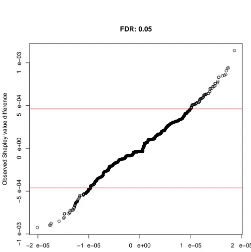
3.5 Test statistics . . . 48
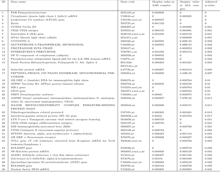
3.6 Analysis of real data . . . 55
3.7 Discussion . . . 57 vii
3.8 Figures and Tables . . . 59
4 Other games on gene expression data 67 4.1 Minimum cost spanning tree and gene expression . . . 67
4.1.1 Preliminary notations . . . 68
4.1.2 MCST situations based on a gene expression data-set . . 69
4.1.3 Future work . . . 76
4.2 Microarray games and the classification problem . . . 77
4.2.1 Future work . . . 80
4.3 Analysis of gene expression data from Real Time PCR . . . 81
4.3.1 Future work . . . 82
A Dichotomization algorithm 85
Chapter 1
Introduction
Nowadays, microarray technology is available for taking ‘pictures’ of gene ex-pressions. Within a single experiment of this sophisticated technology, the level of expression of thousands of genes can be estimated in a sample of cells under a given condition. This monograph deals with the discussion and the application of a methodology based on Game Theory for the analysis of gene expression data. Roughly speaking, the starting point is the observation of a ‘picture’ of gene expressions in a sample of cells under a biological condition of interest, for example a tumor. Then, Game Theory plays a primary role to quantitatively evaluate the relevance of each gene in regulating or provoking the condition of interest, taking into account the observed relationships in all subgroups of genes. To fully understand the methodology introduced in this thesis, some pre-requisites both on Game Theory and on microarray data analysis are required. In order to create a common background for readers who approach for the first time Game Theory or microarray data analysis or both of them, I suggest to look at Sections 1.1 and 1.2, aimed, respectively, to give a basic introduction to cooperative Game Theory and to the statistical analysis of microarray expres-sion data. The contents of those sections are fundamental to understand the objectives of this thesis, which are described in Section 1.3. Finally, in order to understand the theory behind the game theoretical model applied to gene expression data, the preliminary definitions introduced in Section 1.4 and in Section 1.5 are required.
1.1
Introduction to Game Theory
Game Theory is a mathematical theory dealing with models for studying inter-action among decision makers (which are called players). Dealing with decision makers interaction, the reader should be aware that a decision problem that involves only one decision maker is not properly in the domain of application of Game Theory.
Since the seminal book by John von Neumann and Oskar Morgenstern (1944) “Theory of Games and Economic Behavior”, it is usual to divide Game Theory into two main groups of interaction situations (which are called games), non-cooperative and non-cooperative games. Non non-cooperative games deal with conflict situations where non binding agreements among the players can be made. In cooperative games all kinds of agreement among the players are possible.
In non cooperative games, each player will choose to act in his own interest keeping into account that the outcome of the game depends on the actions of all the players involved. Actions by players can be simultaneous (for instance the ‘stone, paper, scissors’ game or the ‘matching pennies’ game) or at several points in time (for instance the game of chess).
Cooperative games deal with situations where groups of players (which are called coalitions) coordinate their actions with the objective to end up in joint profits which often exceed the sum of individual ‘profits’1.
Another important classification in Game Theory about the goals of the analysis performed using its tools. A game, both non-cooperative and cooper-ative, can be analyzed with the objective to indicate what players should do in the game to maximize their profits (usually this goal is referred to as the ‘normative approach’). Another reason for using Game Theory, is to predict the outcome of game, i.e. whether or not players optimize their profits (usually referred to as the ‘predictive approach’).
In this dissertation I focus on the application of cooperative game theory to the analysis of gene expression data from microarray experiments. If it is quite obvious that I do not plan to give advice to genes on how they should behave inside a biological cell, on the other hand it is not so straightforward to figure out how to describe the behavior of genes making them to play a certain game,
1For game theorists, utility value would be more correct than the term profit. As for the
ordinary language, I use for the moment the term profit with reference to something that is in the interest of the decision maker to be maximized.
3 and then use it as a tool to predict which genes obtain the maximum profit.
First, it is not obvious at all what is the meaning of ‘profit’ in this context. In the following sections I will extensively introduce and discuss this topic. However, the possibility to extend the concept of profits, benefits, savings or whatever could be in the interest of each decision maker to be maximized on her/his own count, is a well known feature of Game Theory applications. In Game Theory, the term ‘profit’ usually is more correctly replaced by utility value of a rational player. I do not want to enter here the discussion of how an utility function is defined and why it is a numerical representation of the preferences of a rational decision maker. For introductions to this problem see for instance the books by Kreps (1990) and Osborne and Rubistein (1994).
I will simply note that, sometimes, reasonable considerations bring game theorists to assume that the players preferences are nicely represented just by money, and so money will be the profits to be considered in the game. For example, one can describe a situations using cooperative games in coalitional form where the players are willing to join bigger coalitions in order to have extra monetary benefits or extra monetary savings thanks to the effects of coopera-tion. For instance, consider a cooperative game in coalitional form with three players, 1, 2 and 3, and with a characteristic function v : P({1, 2, 3}) → {0, 1}, where P({1, 2, 3}) is the set of all possible subsets of {1, 2, 3}, and such that each coalition with at least two players get 1 euro, and all the remaining coali-tions get 0 euro (i.e. all the single player coalicoali-tions and the empty coalition get 0). Formally, we are considering the cooperative game in coalitional form ({1, 2, 3}, v) such that v({1, 2, 3}) = v({1, 2}) = v({1, 3}) = v({2, 3}) = 1 and v({1}) = v({2}) = v({3}) = v(∅) = 0 (for this kind of problems see books by Owen (1993), Tijs (2003), Young (1995)).
Other times, preferences of players are not addressed to things that have a monetary counterpart. This is the case, for example, of decisions in a parlia-ment. Assume that there are three parties, A, B and C, which share the seats in parliament by 45%, 40%, and 15%. The preferred outcome for a party or a coalition of parties is intended as the ability to force a decision. In this case, I will say that the coalition is a winning one. Suppose that decisions are made by simple majority. No one of single parties will profit from missing the coopera-tion with others, in the sense that all parties alone are loosing coalicoopera-tions. On the contrary, all coalitions with more than one party inside will be a winning
coalition.
This parliament situation can be properly represented by a cooperative game in coalitional form, where players are the three parties A, B and C and the value of each sub-set of players (coalition) is the label of winning or loosing coalition. Consider 1 as label for winning coalitions, and 0 as label for loosing coalitions. So, only coalitions with at least two players get 1 and the remaining coalitions get 0. We are indeed considering the game ({A, B, C}, w) such that w({A, B, C}) = w({A, B}) = w({A, C}) = w({B, C}) = 1 and w({A}) = w({B}) = w({C}) = w(∅) = 0. Note that this game has precisely the same structure of the game ({1, 2, 3}, v) introduced before. In both cooperative games in coalitional form there are three players (different names, in this case, are not essential), and in both games only coalitions with at least two players get 1, and the others get 0.
What is basically changed, making the ‘same’ game suitable for the de-scription of such completely different situations, is just the definition of the objectives of each coalition in relation to the preferences of its players. In game ({1, 2, 3}, v), it has been assumed that the objective of the players is to maxi-mize their rewards; in terms of preferences it has been assumed that each player prefers 1 euro to nothing. In game ({A, B, C}, w), it has been assumed that the objective of the players is to force a decision in the parliament, so players prefer to have the ability to force a decision than not to have it. Concerning this kind of models, there are many other important aspects that cannot be taken up in a basic introduction on Game Theory. But I think that these very preliminary considerations are already sufficient to give a first insight on the extreme flexibility of the formal definition of cooperative game in coalitional form in representing completely different interaction situations.
Now, some words on what it is possible to predict using cooperative games in coalitional form.
Consider again the example of the parliament. Since the decision rule was the simple majority it seems not very likely that the distribution of power, however defined, coincides with the distribution of seats for parties A, B and C. In order to discuss issues related to the problem of assigning power to the players of similar cooperative games, and understand how the power distribution changes when the number of seats or the decision rule change, classical analytical tools developed in the Game Theory framework are power indices (see for instance
5 Felsenthal and Machover (1998) for a formal discussion of the problem; Owen (1993) for some political applications). The most popular, widely applied to many political institutions (e.g USA President Elections, ONU Council, EU Parliament etc.) are the Shapley-Shubik power index (Shapley and Shubik (1954)) and Banzhaf-Coleman power index (Banzhaf (1965)). Surprisingly, most power indices are nothing else that well known solution concepts for cooperative games in coalitional forms. This means that the same method can be used to allocate among the players the profits of the big coalition in games where the value of each coalition represents, for example, monetary rewards.
Which arguments can support the application of the same solution concept to so different interaction situations and their consequent alternative interpre-tations?
The answer to this question is rooted in the property driven approach2. If the
quantification of power is the goal of the analysis, the property driven approach suggests to postulate discriminating properties which a power measure has to satisfy in order to qualify as an appropriate measure. If the cooperative game concerns monetary profits and the objective is to fairly allocate the total reward of cooperation, of course the basic properties to be postulated can be different and their interpretation must be appropriate to the context. On the strength of the property driven approach, it often happens that a solution concept satisfies sound properties in completely different situations (see for instance the volume by Roth (1988) for different applications of the Shapley value). The strong connection with the property driven approach is in my opinion one of the main reasons of success of applied Game Theory, success which is widely manifested by the several applications of Game Theory to different scientific fields, especially in Economics, Political Science, Social Science and Evolutionary Biology. Next, I will try to convince the reader that it can also be successfully applied to gene expression analysis.
1.2
Introduction to microarray data analysis
Proteins are the structural constituents of cells and tissues and may act as necessary enzymes for biochemical reactions in biological systems. Most genes contain the information for making a specific protein. This information is coded
in genes by means of the deoxyribonucleic acid (DNA). Gene expression occurs when genetic information contained within DNA is transcripted into messenger ribonucleic acid (mRNA) molecules and then translated into the proteins.
Nowadays, a revolutionary technique, i.e., the microarray technology, allows for the collection of huge amount of information concerning the function of human genes. This approach provides a quantitative measure of gene expression (the amount of mRNA in a cell sample) for thousands of genes in the same experiment. The crucial step of this procedure is the hybridization: many DNA regions immobilized on a small glass, plastic or nylon matrix (probes), bind to a complementary sequence from the sample under study (sampled mRNA itself or cDNA obtained by inverse transcription of sampled mRNA), labelled with fluorescent dyes that flag their presence when exposed to a specific wavelength of light. A separate experiment takes place in each of many individual spots arrayed as a regular pattern on the matrix, whence the name array (Parmigiani et al. (2003)).
There are several microarray based technologies, which involve different ex-perimental procedures (see for instance Schena (2003), Parmigiani et al. (2003)). However, a common objective of gene expression microarrays is to consistently generate a matrix of expression data, in which the rows (possibly thousands) index the genes and the columns (usually in the order of units or tens) index the study samples. Numbers in the matrix represent gene expression ratios which quantify the relative expression of genes in one target sample with respect to a given reference sample.
Complex experimental artifacts associated with microarray data collection have been described, emphasizing the need for statistical treatment of data during all stages of the experiment. This includes the design of the slide, the quality assessment, the normalization process (Dudoit et al. (2001); Smith and Speed (2003), Amaratunga and Cabrera (2004)) and other pre-processing data analysis (Amaratunga and Cabrera (2004), Parmigiani et al. (2003)) with the objective of removing systematic variation in microarray experiments. In the following of this paper I will assume to work on a matrix of gene expression values that have been already pre-processed.
Many models for data analysis have been presented in the literature for infer-ring, from a matrix of gene expression data, the role of genes, their interactions and their behavior when changes in condition of the biological system occur
7 (Moler et al. (2000), Su et al. (2003)).
So far, classical statistical techniques used for extracting information from gene expression microarrays can be classified in three main groups: inferential statistical methods used for identifying genes that are regulated by different conditions of interest, e.g., to find single genes or groups of genes which show a statistically significant difference in the expression levels under two or more conditions of interest (Fujarewicz and Wiench (2003), Storey and Tibshirani (2003)); unsupervised analysis techniques, used as a method to identify groups of genes with similar patterns in the expression data (Golub et al. (1999), Alon et al. (1999)); class prediction tools, where selected genes are used to classify samples into known categories of morphology, known biological features, clinical outcomes, or other condition of interests according to gene expression patterns. It is mostly aimed at supporting early diagnosis in new samples (Dudoit and Fridlyand (2003), Golub et al. (1999), Dudoit et al. (2002b)).
In order to give a slightly more accurate idea about how these classical statistical methods have currently been applied to microarray data analysis, I follow the essential outline of the presentation of the methods in what I consider one of the most complete books on microarray analysis at the moment, i.e. the book by Amaratunga and Cabrera (2004).
Concerning the inferential statistical methods, the main task of these meth-ods is usually accomplished by mean of statistical hypothesis testing. The result of an hypothesis testing on a gene expression matrix is its decision among two possible options: to reject the conjecture (null hypothesis) that there is no dif-ferences in terms of gene expression between two conditions of interest or not to reject the null hypothesis and declare that there is insufficient evidence to detect a difference of gene expression between the two conditions. In order to select or develop a good test for a particular microarray data-set, it is necessary to make assumptions about that microarray data-set. Different assumptions for the same situation will generally lead to quite different tests and perhaps even quite different test results. In general it is important to consider assumptions carefully, but this is a very difficult task on microarray analysis where the bio-logical knowledge that could be used as diagnostics to check the assumptions is still vague and strongly dependent from the biological conditions of interest.
Unsupervised analysis techniques, also known as pattern discovery or cluster analysis, has as a main objective to produce evidences for correlated patterns
of gene expression displayed by genes behaving jointly, such as genes perform-ing similar functions or genes operatperform-ing along a genetic pathway. Based on the quantifications of similarity between observations, most of these methods de-pend on either a dissimilarity or similarity measure, which quantifies how far, or how close, two observations (for example vectors of gene expressions across different samples) are from each other. Dissimilarity measures which have been employed in microarray analysis are classical distances like the Euclidean dis-tance (Coco et al. (2005)). It is matter of fact that different definitions of dissimilarity measures bring to different clusters of similar genes. The notion of similarity or dissimilarity used, however, should reflect an a priori selected attribute for joint gene behavior that it is expected to be informative with re-spect to the biological condition under investigation. So far, it is not clear which analytical instruments should be used to evaluate the meaning of a given dissim-ilarity or simdissim-ilarity measure, and the choice of a metric is still almost completely arbitrary.
Finally, few words on supervised analysis, also called class prediction. To better understand the main characteristics of this kind of analysis, I found more explanatory to refer to the biological conditions of interest directly as tumors. In fact, the tumors are known to be of various different classes and a microarray gene expression data-set can be extracted from samples collected from different tumors. Now it is likely that different genes are expressed in the cells of different tumor classes. Therefore it can be conjectured that it ought to be possible to differentiate among the tumors classes by studying and contrasting their gene expression profiles, that is developing a classification rule to discriminate them. The great potential of these methods is that the classification rule could be ex-ploited to predict the class of a new tumor sample of unknown class based on its gene expression profile. Another advantage of these methods is the easy way to evaluate their performance, as the proportion of misclassifications on the gene expression matrix where the original tumor class of samples is known (training set), i.e. the misclassification rate. On the other hand, from the mathematical point of view, the biggest problem in the applications of supervised methods to gene expression data-set is the number of genes much greater than the number of samples. By retaining such a large number of genes, it is incredibly easy for supervised methods to find good-looking but non-reproducible and meaningless classification rules, with low misclassification rate on the training set and very
9 high misclassification rate on the gene expression data where the information on tumor classes is unknown (test set). From this follows the necessity to find a strategy to reduce the number of genes, for example, performing the super-vised procedure only on those genes which result differentially expressed on the basis of the application of inferential statistical methods. Besides the problems concerning the assumptions which affect the statistical inferential methods as I mentioned before, this filtering approach encounters also other disadvantages. Some genes retained could be false positive, and even so produce good perfor-mance as classifiers, perforperfor-mance that of course are not reproducible on other data-set. Even worst, it may exist a set of genes that together acts as a classifier, but each individual gene in the set does not, making them good candidate for being filtered out all together. Moreover, many retained genes could show the same pattern of expression, determining a redundancy in the information.
1.3
Objectives and overview of the thesis
The criterium for the choice of one particular statistical method should be based on the (justified) claim that such method is able to select genes covering the most relevant role in the mechanisms which provoke a biological condition or response of interest (e.g. a tumor). Unfortunately, the big difficulty in taking the decision is that classical statistical methods are not directly related with a biologically sound and operative definition of genes relevance in this context.
Consequently, different sets of genes may be selected depending on the ap-plication of different statistical methods (Jaeger et al. (2003)). Since usually there exists a limit on the number of genes to choose, a researcher might not be able to include all relevant genes in deserving further investigations.
For example, an extremely difficult question to answer is whether a group of genes which are individually differentially expressed between two different conditions are more or less relevant in regulating the mechanisms governing these conditions than another group of genes able to characterize the two con-ditions only jointly. Differently stated, similarly to the considerations done for the classification problem, it may exist a set of genes A that together have a characteristic expression pattern under each condition, but each individual gene in the set has not. On the contrary, it may exist a set of genes B where each individual gene is differentially expressed under the two conditions. So, the
problem is: how to make a quantitative comparison of the roles played by the two respective sets A and B in regulating or provoking the condition of interest? Another very hard practical problem faced when attempting to use a classical statistical method in quantifying genes relevance, is that genes relevance index should take into account the interaction links among genes in the mechanisms which determine the biological condition of interest. This would imply the application of the statistical method to each possible subgroup of thousand of genes, which is often a procedure computationally too costly.
A completely different approach, based on a cooperative game in coalitional form where the players are genes, has been proposed in this thesis.
In my opinion, the novelty of the approach with respect to the classical statistical methods is essentially twofold. First, the class of cooperative games used, called the class of microarray games, provides the effective opportunity to describe the association between the global expression of each coalition of genes and a biological condition of interest and, as a consequence, to incorporate in the successive analysis all possible genes interaction ties related with the biological condition. For example, it is possible to describe the association between the over-expression or the under-expression properties of genes in each coalition and the tumor or the effect of a treatment in samples.
Even considering all possible subsets of genes, which means increasing a lot the level of complexity of the analysis, no strong assumptions on the expression probability distributions have been done. In fact, the characteristic function of a microarray game relays completely on the observed experimental gene expres-sion matrix. The very relevant assumption in this context, is the definition of the causality relation (also called sufficiency principle) which incorporates the criterium used to establish whether the expression levels of genes in a coalition are associated or not with the biological condition of interest.
All the information on genes associations stored in the characteristic function of a microarray game can be successively exploited to quantitatively resume the role of each gene in each possible coalition by means of the application of solution concepts for cooperative games. The second novelty of the approach presented in this thesis is based on this idea of application of solution concepts to microarray games, and on the strong connection between game theory and the property driven approach commonly used for studying the properties of solution concepts. As I pointed out in the general introduction on cooperative game theory, the
11 property driven characterization of solution concepts has abundantly been used in Game Theory, attempting to investigate the real extent of the theory and to contextualize its potential applications.
Usually, the interpretation of the results obtained by classical statistical pro-cedures are strongly dependent from the theoretical model used for the analysis or from strong assumptions about the reference population from which the sam-ples are collected. The property driven approach offers the possibility to over-turn this view: only weak assumptions on the population are needed and what is strongly outlined a priori are the boundaries for a plausible interpretations of the results. In the game theoretical approach, the result is the outcome of a so-lution concept applied to a microarray game built on a gene expression matrix. Its interpretation is contextualized ex-ante by means of sound basic properties, that have to be satisfied by a numerical representation of the role played by each gene in associating the expressions of coalitions with the condition of interest. This view is particular valuable in the genomic field, which is still a relatively young research topic, and the evidences to support strong hypothesis on the reference populations or the application of sophisticated mathematical models are still far from to be clear. These considerations are, in my opinion, effec-tively resumed by the following sentence, in St¨oltzner (2004): if a field is still provisional in its basic concepts, and experience with models is fragmentary, the property driven method is able to act as a controlling instance and steering device for further exploration.
On the other hand, it is not possible to neglect the fact that gene expression is a stochastic, or “noisy”, process (Elowitz (2002), Swain (2002)). Besides the biological noise, microarrays data, as any other experimental process, are subject to random experimental noise. As a consequence, since a microarray game is inferred from gene expression data, a microarray game itself follows a stochastic law. Therefore, I felt the necessity to introduce microarray games in an alternative way, supported by inference arguments, with the objective to assess the effects of the random variability on the observed results of the game theoretical analysis.
Summing up, the class of microarray games and the methods for their anal-ysis, constitute the core of this work. Their intrinsic simple structure was the main reason that convinced me to focus my efforts on their analysis. On the other hand, it is possible that some aspects of the real phenomenon that I was
going to investigate were missed due to the same reason. To catch such aspects, one possibility could be to make the models a bit more sophisticated, and the preliminary study on new classes of gene expression based games is the present direction of my work and the conclusion of my dissertation.
1.3.1
A brief summary of the following chapters
Next sections 1.4 and 1.5 introduce some preliminaries on cooperative games and on microarray data analysis, respectively.
Chapter 2 is based on Moretti et al. (2004), where the class of microarray games has been introduced. Via a dichotomization technique applied to gene expression data, it is constructed a game whose characteristic function takes values on the interval [0, 1]. The objective of such a game is to stress the relevance (‘sufficiency’) of groups of genes in relation to a specific biological condition or response of interest (e.g. a disease of interest). It has been discussed the possibility of applying game-theoretical tools that can take into account the relationships which exist among genes, like the Shapley value. The highest Shapley values of the game should point to the most influential genes, so that it could be useful as a hint for pointing at the genes that mostly deserve further investigation. A property driven characterization of the Shapley value with a genetic interpretation is also provided in order to contextualize and justify the use of the Shapley value as relevance index for genes.
Chapter 3 is based on Moretti (2006). It has been presented a statistical framework aimed at estimating the accuracy of the observed genes relevance index and a procedure to test the null hypothesis of no differences in terms of relevance index for genes studied in samples regulated by different biological conditions. The first goal of Chapter 3 is to answer the question on how accurate are the relevance estimates provided by the Shapley value applied on games introduced in Chapter 2. That question is the prelude for the second subject of this chapter, i.e. comparing the relevance of genes under different biological conditions or responses.
Chapter 4 is still in a germinal form and contains many directions on which I am presently working. In Section 4.1, an alternative model based on minimum cost spanning tree representation of gene expression data has been introduced. One of the main characteristics of this model is the possibility to avoid the dichotomization technique required for microarray games introduced in Chapter
13 2. In Section 4.2, the connections between microarray games and the class prediction problem have been also presented. Finally, in Section 4.3, it has been introduced an overview of analysis performed on gene expression data of neuroblastoma samples that is still in progress and that I am doing using the game theoretical tools presented in the previous chapters.
Finally, note that all the algorithms presented in this dissertation and other procedures used in the analysis of expression data have been implemented using the statistical programming language R (R Development Core Team (2004)), and available on request.
1.4
Preliminary notations on cooperative games
Now, let us introduce some basic game theoretical notations. A cooperative game with transferable utility or TU-game, also known as coalitional game with transferable payoff, is a pair (N, v), where N denotes the finite set of players and v : 2N → IR the characteristic function, with v(∅) = 0. Often we identify
a TU-game (N, v) with the corresponding characteristic function v. A group of players T ⊆ N is called a coalition and v(T ) is called the value of this coalition. A TU-game (N, w) such that w : 2N → [0, 1] is called a [0, 1]-game. We will
denote the class of all [0, 1]-games as W, with W ⊂ G, being G the class of all TU-games (N, v).
Let C ⊆ G be a subclass of TU-games. Given a set of players N , we denote by CN ⊆ G the class of TU-games in C with N as set of players.
The unanimity game (N, uR) based on the unanimity set R ⊆ N is the
game described by uR(T ) = 1 if R ⊆ T and uR(T ) = 0, otherwise. Every
TU-game (N, v) can be written as a linear combination of unanimity games in a unique way, i.e. v =P
S⊆N,S6=∅λS(v)uS (see for instance Owen (1995)). The
coefficients (λS(v))S∈2N\{∅}are called unanimity coefficients or dividends of the
game (N, v).
A TU-game (N, v) is monotonic if for all S, T ⊆ N , S ⊆ T implies that v(S) ≤ v(T ).
Let i ∈ N . For each S ⊆ N \ {i}, the quantity mi(v, S) = v(S ∪ {i}) − v(S)
is the marginal contribution of player i to coalition S. A TU-game (N, v) is convex if for all i ∈ N and all S, T ⊆ N \ {i}, S ⊆ T implies that
An allocation (xi)i∈N of a TU-game (N, v) is a vector in IRN describing the
payoffs of the players, where player i ∈ N receives xi.
An one-point solution for a class C of TU-games is a function ψ that assigns a payoff vector ψ(v) to every TU-game in the class, that is ψ : CN → IRN.
The most famous one-point solution in the theory of cooperative games with transferable utility is the Shapley value, introduced by Shapley (1953). To have a basic idea about the Shapley value, suppose that all the players are arranged in some order, all orderings being equally likely. The Shapley value φiof the game
(N, v) ∈ GN, for each i ∈ N , is defined as the expected marginal contribution,
over all orderings, of player i to the set of players who precede him. Since for each S ⊆ N \ {i} there are precisely (s−1)!(n−s)!n! orderings in which players in S precede player i, than the Shapley value φi applied to game (N, v) ∈ GN can
be calculated by the general formula φi(v) =
X
S⊆N :i∈S
(s − 1)!(n − s)!
n! mi(v, S)) (1.2)
for each i ∈ N , where s = |S| and n = |N | are the cardinality of coalitions S and N , respectively.
An alternative representation of the Shapley value can be given in terms of the unanimity coefficients (λS(v))S∈2N\{∅} of a game (N, v), that is:
φi(v) = X S⊆N :i∈S λS(v) s (1.3) for each i ∈ N .
Another one-point solution for cooperative games with transferable utility is the Banzhaf value, introduced by Banzhaf (1965). The Banzhaf value βi(v)
of a game (N, v) ∈ GN, is defined as follows
βi(v) = X S⊆N :i∈S 1 2n−1mi(v, S), (1.4) for each i ∈ N .
A common characteristics of the Banzhaf value and of the Shapley value of a game (N, v) is that both one-point solutions belong to the class of allocations which can be obtained via the general formula
²i(v) =
X
S⊆N :i∈S
15 where p(S), for each S ∈ 2N \ {∅}, is the probability that a player i ∈ S
joins the other players in S \ {i} to form coalition S. So, ²i(v) is the average
marginal contribution of player i ∈ N with respect to all the possible coalitions in which player i can enter. If p(S) is assumed to be the same for each coalition S ∈ 2N \ {∅}, then p(S) = 1
2n−1, and the definition of the Banzhaf value by
formula (1.4) is obtained. If p(S) is assumed to be dependent from S, one choice could be assume that p(S) = (s−1)!(n−s)!n! , and the definition of the Shapley value by formula (1.2) is obtained. Of course, other probability distributions on the set of all coalitions can be used in order to define different one-point solutions. Finally, a particular set, possibly empty, of allocations of a TU-game (N, v) is the core, which is defined as follows:
core(v) = {x ∈ IRN|X i∈S xi≥ v(S) ∀S ∈ 2N\ {∅}; X i∈N xi= v(N )}.
1.5
Preliminary notations on microarray data
analysis
Let G = {1, 2, . . . , n} be a set of n genes, SR = {1, 2, . . . , r} be a set of r
reference samples, i.e. the set of cells from normal tissues and, finally, let SD=
{1, 2, . . . , d} be the set of d cells from tissues with a biological condition or response of interest (e.g. a disease).
The goal of a microarray experiment is to associate to each sample j ∈ SR∪ SD an expression profile (aij)i∈G, i.e. aij ∈ IR represents the relative
ex-pression value of the gene i in sample j with respect to the reference sample. Globally, such expression values will be indicated as the data set of the microar-ray experiment. In the following we will refer to the data set resulting from the pre-processed method usually called normalization (Dudoit et al.(2001), Smith and Speed (2003)), which allows for comparison among expression intensities of genes from different samples. The data set can be expressed in the form of two expression matrices ASR = (Aj)
j∈SR and A
SD = (Aj)
j∈SD, where the
index here represents a column, i.e. a sample, where the column Aj is the
ex-pression profile on G of sample j. In summary, we will denote as a microarray experimental situation (MES) the tuple E =< G, SR, SD, ASR, ASD >.
As the first step of our analysis, we are interested in understanding whether genes in each sample in SDare abnormally expressed with respect to the
expres-sion values showed in SR according to a certain discriminative criterium. For
example, we could refer to the set of abnormally expressed genes in a sample as the set of over (under) expressed genes in that sample, or the union of over expressed and under expressed genes in that same sample .
We need to introduce useful notation to deal with abnormally expressed genes. Note that gene i ∈ G which results abnormally expressed on a sample j ∈ SDcan be represented setting to 1 the value of a boolean variable bij. We call
abnormal expression profile the vector Bj = (b
ij)i∈G. A discriminant method
can be expressed as a map m assigning to each expression profile from tumor samples a corresponding abnormal expression profile. Hence, all the information on the differences of gene expression of sample in SDfrom the ones of sample in
SR can be represented via an abnormal expression matrix BE,m∈ {0, 1}G×SD.
Since for our purposes the relevant information is contained in the abnormal expression matrix BE,m, in the sequel we identify the MES E and the
discrimi-nant method m with the matrix BE,m. Sometimes, unless otherwise clear from
the context, we will also refer to a boolan matrix B ∈ {0, 1}G×SD as an
abnor-mal expression matrix which has been calculated applying some discriminant method m to some MES E.
Example 1 Consider an MES E =< G, SD, SR, ASD, ASR > such that ASR is
reported in the following table
sample 1 sample 2 sample 3 sample 4
gene 1 0.4 0.2 0.3 0.6
gene 2 12 10 4 5
gene 3 8 13 20 9
gene 4 0 -0.5 1.4 1.1
and ASD is given in the following one
sample 1 sample 2 sample 3
gene 1 0.9 0.4 0.7
gene 2 4.6 15 18
gene 3 7 21 12
17 Note that also negative values are possible. This is due to the fact that, usually, in literature the data set of a microarray experiment is presented in terms of the logarithm of the relative gene expression ratios, i.e, gene expression in the target sample / gene expression in the reference sample. Consequently, a positive number indicates a higher gene expression in the target sample than in the reference one, whereas a negative number indicates a lower expression in the target sample.
Now consider a very naive discriminant method m for the two classes 1 and 0, where 1 labels abnormally expressed genes and 0 labels normally genes and such that (m(Aj, ASR)) i = 1 if Aji ≥ maxj∈{1,...,|SR|}A SR ij or A j i ≤ minj∈{1,...,|SR|}A SR ij 0 otherwise.
Then the corresponding abnormal expression matrix is the following
BE,m= 1 0 1 0 1 1 1 1 0 0 0 1 .
Chapter 2
The class of Microarray
games and the relevance
index for genes
2.1
Introduction
Aim of this chapter is to address the problem of quantifying the relative rel-evance of genes in a complex scenario - such as the pathogenesis of a genetic disease - on the basis of the information provided by microarray experiments, and taking into account the interaction level of each subgroup of genes.
In analyzing gene-gene relationships in microarray data, the main difficulty is the impossibility to obtain, trough pre-processing data analysis, a total elim-ination of the technical and biological bias. For this reason, in our approach we refer to the observed average interaction level of a group of genes, i.e., the aver-age number of tumor samples in which such a group of genes can be considered responsible, according to a pre-defined causality principle, for the onset of the tumor: the higher is the number of samples observed, the lower is the proba-bility that chance could affect the inferences provided by the model. The basic idea of this model comes from the theory of cooperative games with transferable utility (TU-games). In particular we considered the framework of simple games, which have been widely applied to the analysis of the power of players in
tion situations as Councils, Parliament, etc. (Owen (1995), Shapley and Shubik (1954), Banzhaf (1965)). We adopted the same formal language of TU-game for modelling the interaction among genes, considered as players, in relation to the pathogenesis of a genetic disease, e.g., a tumor. The game we considered origins from the comparison of two matrixes of gene expression data; one from tumor samples and the other from normal DNA (referent healthy subjects). We first used a discriminant method on each sample to split the whole set of genes in two sets, i.e., those genes showing an expression ratio largely different from normal samples, and those with expression levels corresponding to normal DNA samples. At this preliminary stage of the model, for each single gene, as in detail explained in Section 1.5, we used the interval boundaries containing most data in the normal distribution of that gene as cut-offs for discrimination (Becquet et al.(2002)). We then introduced a causality relation (also called sufficiency principle) which directly determines the characteristic function of the game. An interpretation of the biological meaning of a relevance index, used for measuring the “power” of each gene in inducing the tumor, has been given and it turned out to coincide with the Shapley value of the game considered.
In Section 2.2 the class of microarray games is introduced starting from the general notion of the sufficiency principle, and some basic properties and exam-ples of such games are reported. In Section 2.3 an axiomatic characterization of the Shapley value is given by means of five properties suitable to genetic interpretation of this index. Section 2.4 concludes with some considerations on related works and future research.
2.2
Interaction among genes
In this phase of the analysis we assume that the abnormal expression profile Bj,
for each sample j ∈ SD, is a sufficient conditions for the onset of the disease (or
another biological condition or response of interest) in individuals from which samples in SD are collected (sufficiency principle for groups of genes). Stated
differently, a group of genes A ⊆ G which are abnormally expressed in a sample of SD(according to a discriminant method m applied to the reference expression
matrix ASR) implies that an individual whose sample has at least all (possibly
21 in G abnormally expressed (again on the basis of m and ASR) should have the
disease.
One could wonder why a microarray experiment can show -as it usually happens- different groups of abnormally expressed genes in different tumor sam-ples.
We attempt to provide an answer to such a question with arguments coming from different directions.
One is dealing with biology: it is in fact likely that early stages of car-cinogenesis involve metabolic paths which are controlled by different groups of genes.
Another reason is technical: a microarray experiment can be affected by many sources of noise (Parmigiani et al.(2003), Smith and Speed (2003)) and this unwanted variability can affect the measurement of expression values. Despite the reduction of variability in microarray experiments has been the objective of several works in the last few years, in practice the likely misclassification of some genes considered as abnormally expressed cannot be avoided, due to technical uncertainty.
The arbitrariness of methods used for the discriminant analysis should also be considered, i.e. the structure of the sufficient groups can be easily biased by a bad choice of the discriminant method.
The aim of this work is to give an answer to the following questions: how much relevant for the onset of a tumor are the genes which are abnormally expressed inside the sample SD? Is it possible to provide a measure of the
power of genes in determining the onset of the tumor in an individual, on the basis of the information collected via samples SD and SR and the discriminant
method m used?
Consider for instance a MES ¯E =< G, SD, SR, ASD, ASR > and a
discrimi-nant method m such that the corresponding abnormal expression matrix is
BE,m¯ = 1 1 1 0 0 0 1 1 1 0 0 0 . (2.1)
On the basis of matrix (2.1) it seems very reasonable to affirm that on the basis of the information collected ASR and the discriminant method used m,
all the genes abnormally expressed have the same power in causing the tumor, assuming the principle of sufficiency for groups of abnormally expressed genes introduced before.
On the other hand, it could be reasonable to expect experimental situations where there are many abnormal expression profiles inside the sample SD, like
in the abnormal expression matrix of Example 1 and Example 2.
Example 2 Consider again the MES E of Example 1 and a more conservative discriminant method ¯m such that
( ¯m(Aj, ASR)) i= 1 if Aji ≤ p25% i or A j i ≥ p 75% i 0 otherwise.
The resulting abnormal expression matrix is the following
BE,m¯ = 1 0 1 1 1 1 1 1 0 0 1 1 .
where p25%i and p75%i are the 25th and the 75th percentiles of the expression distribution of gene i (i.e. the ith row) in the reference expression matrix ASR,
for each i ∈ G.
How to deal with these situations?
Given an MES E =< G, SD, SR, ASD, ASR > and a discriminant method m,
first we determined the average number of individuals with the tumor due to the abnormal expression of a given group of genes. Of course we calculated such average values on the basis of the information provided by the pair < E, m >, that is, for each group A ⊆ G, we looked at the number of groups of abnormal expressed genes in BE,m that are included in A. We formalize such a concept
via the following definitions (in the following BE,m(j) will be the column j,
j ∈ {1, . . . , |SD|}, of the abnormal expression matrix BE,m).
Definition 1 Let v ∈ {0, 1}n, n ∈ {1, 2, . . .}. We define the support of v
denoted by sp(v) the set
23 Example 3 Consider the abnormal expression matrix BE,m of Example 1.
Then sp(BE,m(1)) = {1, 3}, sp(BE,m(2)) = {2, 3} and sp(BE,m(3)) = {1, 2, 4}.
Definition 2 Let E =< G, SD, SR, ASD, ASR > be an MES and let m be a
discriminant method. We define the average number of individuals with tumor determined by the genes in G, for each T ∈ 2G\ {∅} as the value
v(T ) = |Θ(T )| |SD|
(2.2) where |Θ(T )| is the cardinality of the set
Θ(T ) = {k ∈ {1, . . . , |SD|} | sp(BE,m(k)) ⊆ T, sp(BE,m(k)) 6= ∅} (2.3)
and v(∅) = 0.
Now, the definition of the corresponding TU-game should be clear: • the set of players is the set of genes G;
• the characteristic function is the average number of individuals with tumor determined by the genes T , for each T ∈ 2G\ {∅}.
More formally
Definition 3 Let E =< G, SD, SR, ASD, ASR > be an MES and let m be a
discriminant method. We define the corresponding microarray game as the TU-game (G, v), where v is defined as in Definition 2.
Remark 1 Condition sp(BE,m(k) in relation (2.3) is due to practical
consid-erations concerning the interpretation of the sufficiency principle for groups of genes on samples where genes do not show any abnormal expression properties. We are assuming that the contribution of such a sample in increasing the level of association between the abnormal expression of genes in S and the disease (or another condition of interest) is null, for each coalition S ⊆ N .
The class of microarray games will be denoted with the symbol M. Let E =< G, SD, SR, ASD, ASR > be an MES and let m be a discriminant method.
Ac-cording to equality (2.2), an equivalent way to calculate the corresponding mi-croarray game v is as a sum of unanimity games as follows
v = 1 |SD|
X
j∈{1,...,|SD|}
where usp(BE,m(j)) is the unanimity game on sp(BE,m(j)) ⊆ G, for each j ∈
{1, . . . , |SD|}.
Alternatively, it is possible to rewrite equation (2.4) in terms of the unanimity coefficients of a microarray game v. Let ¯λS ∈ {0, 1, 2, . . .} be the number of
occurrences of the coalition S as support in the abnormal expression matrix BE,m. In formula v = 1 |SD| X S⊆N :S6=∅ ¯ λSuS. (2.5)
where ¯λS = |{k ∈ {1, . . . , |SD|} s.t. sp(BE,m(k)) = S, sp(BE,m(k)) = ∅}|.
Example 4 Consider again the abnormal expression matrix BE,mof Example
1 By equation 2.4 the corresponding microarray game ({1, 2, 3, 4}, v) is such that v =1 3¡u{1,3}+ u{2,3}+ u{1,2,4}¢. It follows that v(∅) = v({1}) = v({2}) = v({3}) = v({4}) = v({1, 2}) = v({1, 4}) = v({2, 4}) = v({3, 4}) = 0; v({1, 3}) = v({2, 3}) = v({1, 3, 4}) = v({2, 3, 4}) = v({1, 2, 4}) = 13; v({1, 2, 3}) = 23, v({1, 2, 3, 4}) = 1.
It is easy to check that microarray games are [0, 1]-games.
At this point, the major fundamental question addressed by our work can be formulated in the following terms: is it possible to employ the standard theory of TU-games to measure the expected relevance of each gene in determining the onset of tumor on the basis of the microarray experimental situation and the discriminant method used?
For instance, we can calculate the Shapley value of a microarray game. In the last fifty years, many studies have addressed the goal of evaluating the power of players (e.g. members of councils, voters in an electoral systems, parties in a parliament etc.) (see for instance Owen (1995)), which are TU-games whose characteristic function can only assume values 1 (for winning coalitions, i.e. coalitions which are able to force the endorsement of a motion) or 0 (for loosing coalitions). In such contexts, the idea was to evaluate the amount of power of players according to the role covered by each of them in supporting the goal of each possible coalition. There, the Shapley value (Shapley (1953), Shapley and Shubik (1954)), as well as many other solutions for TU-games, have been interpreted as power index for players (Shapley and Shubik (1954), Banzhaf (1965)).
25 On the other hand, even if the Shapley value has been proved to be very meaningful in political applications, it cannot be taken for granted the same significance in the microarray context.
The next examples show the behavior of the Shapley value on some particular instances of microarray.
Example 5 The Shapley value of the microarray game in Example 4 is ( 5
18, 5 18, 1 3, 1
9). This means that on the basis of the corresponding MES E and the
discriminant method m the Shapley value of the microarray game states that the most important attribute in determining the tumor onset - on the average - is gene 3, followed by genes 1 and 2 with the same score and gene 4.
Example 6 The Shapley value of the microarray game corresponding to the abnormal expression matrix in Example 2 is (29,13,29,29). On the basis of the considerations detailed in Example 5, we obtain that the most important gene in determining the tumor onset, on the average, is gene 2, followed by gene 1, 3 and 4 with the same score.
Example 7 Consider again the abnormal expression matrix (2.1). The Shapley value of the corresponding microarray game is (1
2, 0,
1 2, 0).
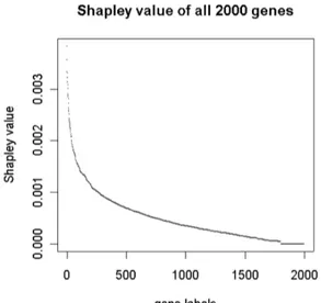
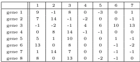
Example 8 We introduce here a preliminary application of our model on a real MES Ec =< G, SD, SR, ASD, ASR > where ASD and ASR represent the
tumor/normal data set (freely obtainable on the web site1) containing
expres-sion levels of a set G of 2000 genes measured using Affymatrix oligonucleotide microarrays for a set SDof 40 tumor samples and a set SRof 22 normal samples
of colon tissues. After the preprocessing stage performed by the Bioconductor specific software for microarray analysis (Gentleman et al.(2004)), we applied the discriminant method m introduced in Example 1 in order to provide the abnormal expression matrix BEc,m, which finally produces the corresponding
microarray game (G, vc).
In the following Table, the first ten genes with highest Shapley value2 on
the microarray game (G, vc) have been indicated.
1http://microarray.princeton.edu/oncology/affydata/index.html 2We computed the Shapley value of the microarray game (G, v
c) by means of the procedure
suggested by equation (1.3), implemented in the programming language R (R Development Core Team (2004)). Also the discriminant methods and other procedures for the manage-ment of data sets used in this application have been implemanage-mented using the language and environment R.
Gene Gene Name Shapley
Number ×(10−3)
Z50753 H.sapiens mRNA for GCAP-II/ 3.83
uroguanylin precursor
H17434 NUCLEOLIN (HUMAN) 3.56
H06524 GELSOLIN PRECURSOR, PLASMA (HUMAN) 3.34
H72234 DNA-(APURINIC OR APYRIMIDINIC SITE) 3.33
LYASE (HUMAN)
M36634 Human vasoactive intestinal peptide (VIP) 3.23 mRNA, complete cds.
U06698 Human neuronal kinesin heavy chain mRNA, 3.21 complete cds.
H61410 PLATELET GLYCOPROTEIN IV (H. sapiens) 3.14
R39209 HUMAN IMMUNODEFICIENCY VIRUS TYPE I 3.13
ENHANCER-BINDING PROTEIN 2 (H. sapiens)
M58050 Human membrane cofactor protein (MCP) 3.09 mRNA, complete cds.
H08393 COLLAGEN ALPHA 2(XI) CHAIN (H. sapiens) 3.01 The complete distribution of the Shapley value on the genes is depicted in Figure 1.
Some of the genes selected were previously observed to be associated with the colon cancer (Fujarewick and Wiench (2003)): the vasoactive intestinal peptide (VIP), has been suggested to promote the growth and proliferation of tumor cells; the membrane cofactor protein (MCP) represents a possible mechanism of the ability of the tumor to evade destruction by the immune system (tumor escape); gelsolin is protein which acts as both a regulator and an effector of apoptosis, i.e. the mechanism responsible for the physiological deletion of cells. DNA-apurinic or apyrimidinic site lyase protein plays an important role in DNA repair and in resistance of cancer cells to radiotherapy (Moler et al.(2000)).
For comparison, we computed on the corresponding microarray game also another very famous solution: the Banzhaf value (Banzhaf (1965)). The com-mon genes in the top ten of Shapley value and Banzhaf value have been indicated in bold.
27
Figure 2.1: Shapley value of genes in a real MES.
The previous examples show a reasonable behavior of the Shapley value in measuring the relevance of each gene in determining the tumor onset. Further-more, to support the idea that the Shapley value is a good estimator of the relevance of each gene, in the next section we provide a new axiomatic charac-terization of this solution satisfying properties which have a nice interpretation in the gene scenario.
We end this section with some properties of microarray games.
Proposition 1 Let < G, SD, SR, ASD, ASR > and m be an MES and a
dis-criminant method, respectively, and let v be the corresponding microarray game in MG. Then v is a super-additive, monotone and convex TU-game.
Proof Super-additivity and monotonicity follow directly from the fact that unanimity games are super-additive and monotone and by equation (2.5) mi-croarray games are positive linear combination of unanimity games.
It is easy to check that Convexity follows analogously from convexity of unanimity games. First, note that for an unanimity game uS, S ⊆ N , the
marginal contribution uS(T ) − uS(T \ {i}) can be 0 or 1, for each i ∈ N and
each T ∈ 2N \ {∅} such that i ∈ T . If i ∈ N \ S, then u
S(T ) − uS(T \ {i}) = 0.
statement:
uS(T ) − uS(T \ {i}) = 1 ⇒ uS(R) − uS(R \ {i}) = 1
holds for each R, T such that T ⊆ R ⊆ N and i ∈ T . Hence, it remains to prove equation (1.1) on game uS.
Again, convexity of v follows immediately by equation 2.5, since for each T ⊆ R ⊆ N \ {i} and each i ∈ N
v(T ∪ {i}) − v(T ) = 1 |SD| P S⊆N :S6=∅λ¯VuV(T ∪ {i}) −|S1D|PS⊆N :S6=∅¯λVuV(T ) = 1 |SD| P S⊆N :S6=∅λ¯V¡uV(T ∪ {i}) − uV(T )¢ ≤ 1 |SD| P S⊆N :S6=∅λ¯V¡uV(R ∪ {i}) − uV(R)¢ = v(R ∪ {i}) − v(R), where ¯λS = |{k ∈ {1, . . . , |SD|} s.t. sp(BE,m(k)) = S}|.
2.3
An axiomatic characterization of the
Shap-ley value with genetic interpretation
In order to characterize the Shapley value by means of properties with genetic interpretation, the definition of partnership of genes takes a basic role.
Definition 4 Let v ∈ MN. A coalition S ∈ 2N\ {∅} such that for each T ( S
and each R ⊆ N \ S
v(R ∪ T ) = v(R) is a partnership of genes in the microarray game v.
The worth v(S) of a partnership of genes S represents the maximum average number of onsets of the tumor that genes in the partnership are able to deter-mine in the population, whatever the interaction of its genes with the others outside the partnership may be. Note that the concept of partnership in TU-games has been introduced in Kalai and Samet (1988) in a general context not involving genes.
29 Remark 2 Let v ∈ MN and let S ∈ 2N\ {∅} be a partnership in v. Then it is
trivial to prove that each T ⊆ S is a partnership itself.
Let v ∈ MN. A maximal partnership S ∈ 2N\ {∅} in v is a maximal subset of
N with the property to be a partnership in v.
We denote by P(v) the set of all the maximal partnerships in v. Note that, by Definition 4, it immediately follows that all one player coalitions are partnerships in v. One easily obtains that the collection of maximal partnerships in v forms a partition of N . For instance, in the microarray game ({1, 2, 3, 4}, v) of Example 4 P(v) = {{1}, {2}, {3}, {4}} and coincides with set of all the partnerships in v; whereas in the microarray game of Example 7 P(v) = {{1, 3}, {2, 4}}.
Some interesting properties for solutions of microarray games, which are related to the concept of partnership of genes, are the following.
Let F : MN → IRN be a solution on the class of microarray games.
Property 1 Let v ∈ MN. The solution F has the Partnership Rationality
(PR) property, if
X
i∈S
Fi(v) ≥ v(S)
for each S ∈ 2N \ {∅} such that S is a partnership of genes in the game v.
The PR properties determines a lower bound of the power of a partnership, i.e. the total relevance of a partnership of genes in determining the onset of the tumor in the individuals should not be lower than the average number of cases of tumor enforced by the partnership itself.
Property 2 Let v ∈ MN. The solution F has the Partnership Feasibility (PF)
property, if
X
i∈S
Fi(v) ≤ v(N )
for each S ∈ 2N \ {∅} such that S is a partnership of genes in the game v.
On the contrary of PR, the PF properties determines an upper bound of the power of a partnerships, i.e. the total relevance of a partnership of genes in determining the tumor onset in the individuals should not be greater than the average number of cases of tumor enforced by the grand coalition, which is always 1.
Property 3 Let v ∈ MN. The solution F has the Partnership Monotonicity
(PM) property, if
Fi(v) ≥ Fj(v)
for each i ∈ S and each j ∈ T , where S, T ∈ 2N\ {∅} are partnerships of genes
in v such that S ∩ T = ∅, v(S) = v(T ), v(S ∪ T ) = v(N ), |S| ≤ |T |.
The PM property is very intuitive: consider two disjoint partnerships of genes enforcing the same average number of cases of tumor in the set of samples. If the genes outside the union of those two partnerships are irrelevant - that is they do not contribute in increasing the average number of tumors - then genes in the smaller partnership should receive a higher relevance index than genes in the bigger one.
The next two properties do not involve the concept of partnership of genes. Property 4 3 Let v
1, . . . , vr ∈ MN. The solution F has the Equal Splitting
(ES) property, if F ( Pr i=1vi r ) = Pr i=1F (vi) r .
Remark 3 Note that
Pr
i=1vi
r ∈ M
N.
Moreover, if BEi,m
1 , . . . , BErr,m are r abnormal expression matrix with the
same number of columns and v1, . . . , vr∈ MN are the corresponding microarray
games, thenPri=1vi
r coincides with the microarray game corresponding to the
ab-normal expression matrix obtained juxtaposing the matrices BEi,m
i , . . . , BErr,m.
To prove these facts a cumbersome notation is needed. So, we prove it in detail only for r = 2.
Let k, l, p ∈N and let ⊕ : IRk×l× IRk×p → IRk×(l+p) be a matrix operator
such that if A ∈ IRk×l and B ∈ IRk×p, then A ⊕ B = C is such that Ci = Ai
for each i ∈ {1, . . . , l} and Cj+l= Bj for each j ∈ {1, . . . , n}.
Let AEA,m∈ {0, 1}k×l and BEB,m∈ {0, 1}k×p be two abnormal expression
matrix arising from the application of a given discriminant method m on two different microarray experimental situations on the same set of genes G and the same set of reference samples SR, with |G| = k, and where l and p are the
cardi-nality of the respective sets of tumor samples. Consider vA, vB∈ MN the two
3Assuming the continuity of F , it can be proved, using functional equation theory, that
the ES property is equivalent to the simpler property of requiring that F satisfies F (v+w 2 ) = F(v)+F (w)
2 for each pair v, w ∈ M N.
31 corresponding microarray games, respectively obtained from AEA,mand BEB,m
by Definition 3. It is easy to check that the game vA+vB
2 is the microarray game
corresponding to the abnormal expression matrixLp
i=1AEA,m⊕
Ll
i=1BEB,m.
Therefore, if l = p, the microarray game vA+vB
2 corresponds to AEA,m⊕BEB,m.
For r > 2 similar arguments hold too.
The ES property underlies a principle of equivalence of reliability levels for microarray games arising from equal splitting of the same MES. Let < G, SD, SR, ASD, ASR> be an MES and let SD1, . . . , SDm form a partition of the
set of samples SD such that |SD1| = |SD2| = · · · = |SDm|. If the ES property
holds, then the relevance index computed on the microarray game correspond-ing to < G, SD, SR, A, ASD, ASR > equals the average of the relevant indices
computed on the microarray games arising from the microarray experimental situations < G, SD1, SR, A
SD1, ASR >, . . . , < G, S
Dm, SR, A
SDm, ASR >,
re-spectively; differently stated, the relevance index is independent from the equal splitting partition {SD1, . . . , SDm} chosen.
The last property involves the definition of null player of a game (N, v), that is a player i ∈ N such that v(S ∪ i) = v(S) for each S ⊆ N \ {i}.
Property 5 Let v, w ∈ MN. The solution F has the Null Player (NP)
prop-erty, if for each null player i ∈ N
Fi(v) = 0.
The interpretation of the NP property is straightforward: if a player does not contribute anything to each coalition S ∈ 2N then he gets null relevance.
Remark 4 It is well known in literature that the Shapley value satisfies the NP property on each class of TU-games CN ⊆ GN. The ES property directly
follows from Remark 3 together with additivity and homogeneity of the Shapley value φ on GN, that is φ(αv + βw) = αφ(v) + βφ(w) for each v, w ∈ GN.
Lemma 1 Let v ∈ MN and let S ∈ 2N \ {∅} be a maximal partnership in v.
Proof Let φ(v) be the Shapley value on the game v. For each U ⊆ N such that i ∈ U the marginal contribution of player i ∈ S is the following
v(U ) − v(U \ {i})
= v([U ∩ S] ∪ [U \ S]) − v([(U ∩ S) \ {i}] ∪ [U \ S]) = v(U \ S) − v(U \ S) if U ∩ S 6= S v(U ) − v(U \ S) if U ∩ S = S = 0 if U ∩ S 6= S v(U ) − v(U \ S) if U ∩ S = S,
where the second equality follows by Definition 4 on partnership S.
Then, the marginal contribution of each player i ∈ S to coalition U is dif-ferent from zero only if S is a subset of U , which means that by equation (1.2) the Shapley value of player i is
P
U⊆N :i∈U (u−1)!(n−u)!n! (v(U ) − v(U \ {i}))
=P
U⊆N :S⊆U
(u−1)!(n−u)!
n! (v(U ) − v(U \ S)),
for each i ∈ S, proving that the Shapley value is the same for each player i ∈ S.
Lemma 2 Let v ∈ MN and let S ∈ 2N \ {∅} be a maximal partnership in v.
Then
v(U ) = 0 for each U( S.
Proof Suppose on the contrary v(U ) 6= 0. Then, by Definition 3, v(R ∪ U ) > v(R) for each R ⊆ N \ U , which yields a contradiction by Definition 4.
Proposition 2 The Shapley value satisfies the properties PM, PR, PF. Proof Let v ∈ MN and let φ(v) be the Shapley value on the game v.
33 i) Let S and T two disjoint partnerships such that v(S) = v(T ) and v(S ∪
T ) = v(N ).
If S and T are subsets of the same maximal partnership, then their Shapley index is the same by Lemma 1, and PM is directly satisfied.
If S and T are subsets of two different maximal partnerships U and V , respectively, then S = U and T = V . In fact, suppose on the contrary that S ⊂ U or T ⊂ V . By condition v(S) = v(T ) and Lemma 2 we have v(S) = v(T ) = 0, and then, by definition 3, it follows v(S ∪ T ) 6= v(N ), which yields a contradiction.
We still have to prove PM when S and T are two maximal partnerships. By condition v(S ∪ T ) = v(N ) and Definition 3, it turns out that v(U ) = v(U ∩ (S ∪ T )) for each U ⊆ N . By Lemma 2 and Definition 4 v(R) = 0 for each R ⊆ S ∪ T , with S, T* R. Hence, it is possible to write the game v in terms of unanimity games in the following way
v = 1 |SD|
¡v(S)(uT + uS) + v(N )uS∪T¢,
where SDis the number of samples in the corresponding MES. Finally, by
equation 1.3, φi=v(S)|S| +|S|+|T |v(N ) for each i ∈ S and φj= v(S)|T | +|S|+|T |v(N ) for
each j ∈ T , which concludes the proof of the PM property of the Shapley value.
ii) The convexity of microarray games by Proposition 1 guarantees that the Shapley value φ(v) is in the core of the microarray game v. The PR property follows directly from intermediate rationality of core allocations. iii) For each S ∈ 2N \ {∅} such that S is a maximal partnership in v, by
monotonicity of v and the fact that φ(v) is in the core of the microarray game v we haveP
i∈Sφi(v) ≥ v(S) ≥ 0. On the other hand, by efficiency
of the Shapley value,P
i∈Nφi(v) = v(N ) and then Pi∈Sφi(v) ≤ v(N ),
which proves that the Shapley value satisfies the PF property.
Theorem 1 Let be given a finite set N . The Shapley value on the class MN
of microarray games is the unique relevance index which satisfies the properties PR, PF, PM, ES and NP.