CARME Conference
(Correspondence Analysis and Related MEthods) Invited talk, Rennes, February 2011
Some Comments on Correspondence Analysis.
P. CAZES
CEREMADE, Université Paris Dauphine I Introduction
II Data analysis as an experimental science
III The Laboratory of Statistics of University Paris 6 in the seventies IV Coding
IV 1 Usual Coding
IV 2 Coding allowing obtaining the equivalence with other analyses IV 2.1 Case of Principal Component Analysis
IV 2.2 Analysis with respect to a model
V Correspondence analysis as a particular case of other methods VI The multiple table analysis ([Caz04])
VI 1 General principles
VI 2 Case where It = I and Jt = J are independent of t (ternary tables kIJT)
VI 2. 1 Classical analysis
VI 2. 2 Deeper analysis: interactions study
VII Ascendant Hierarchic Classification and correspondence analysis VIII Correspondence analysis and classical statistics
IX Correspondence analysis and modelling techniques
IX 1 The reconstitution formula considered as a modelling technique
IX 2 Correspondence analysis and log- linear models in the multiple table case IX 3 Correspondence analysis as an intermediate step in a modelling problem
X Factorial analysis use in the work area XI Bibliography
I Introduction
After having recalled in paragraph II why correspondence analysis (CA) and more generally Data Analysis can be considered as an experimental science, we will analyze in paragraph III the activity of the Laboratory of Statistics of Professor Benzécri at University Pierre et Marie Curie (Paris 6) in the seventies and the eighties, and in particular the Master of Statistics and the publications that have been released. We will then come back in paragraph IV on the importance of coding in CA, and especially fuzzy coding and coding allowing obtaining the equivalence between CA and other analyses. In paragraph V, we recall that CA is a particular case of numerous classical analyses, while in paragraph VI, we will detail the case of multiple tables. In paragraph VII, we will speak about the links between ascending hierarchical classification and CA. Then, we will analyze in paragraph VIII the links between CA and classical statistics. In paragraph IX, we show interest of CA in certain modelling problems whilst paragraph X treats briefly of the use of CA in the working environment. At last, the paragraph XI gives the bibliography.
We didn’t try to be exhaustive in this presentation. We just highlight some important points on CA without quoting all the possible references on a given subject.
II Data analysis as an experimental science
We can consider at a certain level Data Analysis as an experimental science. First, some theoretical results have been discovered and demonstrated after having been observed on the computer listings. Secondly, some indices (inertia rates, contributions, etc) have been set-up to validate the results read at the computer outputs, and we can link with the errors computation in physics. Finally, coding techniques allowing defining the ad-hoc table to be analyzed and the succession of the analyses (descriptive, explicative or decisional analyses) to be done to treat the data and solve a problem is analogous to the setup of an experiment in physics.
I will come back more in details on the theoretical results found experimentally quoting three examples.
B. Escofier demonstrated during his PhD thesis, and after having seen it on the listings, that in the case of the contingence table crossing two sets I and J, the inertia moments of the clouds NI and NJ associated respectively to I and J are equal, result which is now standard. In the
same way, she shown that the factors on I and J coming from the analysis of the cloud NIXJ of
the couples was the same than those obtained in the separated analysis of NI and NJ [Ben 82].
In June 1971, Pr. Benzécri having suggested to Mrs. Bara to do CA of a doubling table of 0 and 1, she discovers with J.P. Pagès that this analysis was equivalent to the Normed Principal Component Analysis of the non doubling table. If this result would not has been observed experimentally (same factorial plans in the two analyses), I doubt someone would have try to demonstrate it.
Identically, in 1971, J.P. Nakache came one day to the Laboratory of Statistics, having analyzed a table of 0 and 1 (in fact a complete disjunctive table) and showed to Professor Benzécri that he obtained interesting and interpretable graphics. Starting from that and also of a note of L. Lebart ([Leb71]), Pr. Benzécri explained in the polycopied Bin. Mult. (published later in the Cahiers de l’Analyse des Données [Ben 77]) why the obtained results were interesting on a practical point of view by showing the equivalence between CA of the complete disjunctive table and CA of the Burt table. This produces an exercise for the exam of the Master of Statistics and then contributed to the development of multiple correspondence analysis (MCA).
I do not insist on the validation problems that in addition to the indices defined to interpret the factorial axes or the classes coming from a classification, have been strongly developed with the improvement of the computer progress, in particular the storing possibilities and the CPU increase (bootstrap, simulation, etc…). I just recall that L.Lebart has deeply contributed to these validation methods and mention only his paper [Leb.06] where bootstrap is in particular used.
Finally, since they are very important, we will speak in paragraph IV about the coding problems.
III The Laboratory of Statistics of University Paris 6 in the seventies
During those years, Professor Benzécri was director of the Laboratory and also responsible of the Master of Statistics. This Master had between 100 and 200 students, which made it the greatest of France, with respect to the number of students. Starting in 1974, about 40 PhD have been defended each year, about 15 being defended in June and at the beginning of July, where there were about three or four defenses each Monday.
Numerous examples of application in various fields were treated: Biology, ecology, economy, geology, linguistics, medicine, physics, psychology, sociology, etc… The diversity of student’s origin was very important: French, of course, but also African, Argentinean, Greek, Egyptian, Iranian, Irish, Libanian, Syrian, Turk, Vietnamese, etc….
This was the source of great discussions and numerous ideas, and results in the exceptional impact of the Laboratory. This has been concretized with the publication, in 1973, of the two famous books on Data Analysis ([Ben73]) which used most of the studies done in the Laboratory between 1968 and 1973, and also the Master’s lectures. The creation, in 1976 of the ‘‘Cahiers de l’Analyse des Données’’ (CAD) allows from one side to complete the books with theoretical article on regression, discriminant analysis, multiple correspondence analysis, and from the other side, to give a synthesis of the PhD thesis defended in the Laboratory. Then, the publication of the books of the collection “Pratique de l’Analyse des Données” begins in 1980, with a book on CA [Ben 80], followed by a book treating of model cases [Bas80] and giving, with a short lecture recall, an important number of exams of the Master of Statistics, with their solutions. The third book [Ben 81] published in 1981 was related to linguistics, while the two last one, talking about medicine [Ben 92b] and economy [Ben 86], where published later. One can notice that those two last books used essentially papers published in CAD and that the first book has been translated in English by Gopalan ([Ben 92a]). I would like finally to quote the book of Pr. Benzécri on the History and Prehistory of Data Analysis published in 1982 after its publication in four articles in CAD.
I would like also to quote the two days colloquiums, usually very friendly and productive, that have been housed by numerous French universities starting in 1970: Besançon, Marseille, Nice, Rennes, l’Arbresle near Lyon, etc…
IV Coding
IV 1 Usual coding
Coding plays a fundamental role in data analysis, and in particular in CA to define the tables to be analyzed.
Among the classical coding, we can quote the doubling of a table of data (case of a table of notes, of ranks, of 0 and 1, etc…), the complete disjunctive coding, and the fuzzy coding. This last coding was the source of many papers in CAD between 1980 and 1990: barycentric coding at 3 or r modalities of a quantitative variable, coding allowing to get rid of the subject
personal equation when the subjects give a certain number of notes, etc… A synthesis of those coding is given in [Caz90].
In the exchange table kIJ where I = J designates for example a group of countries, and where
the general term of the table k(i, j) is equal to the total of the importations from i to j, it is usual to analyze the table (kIJ , kJI), juxtaposition of the table kIJ and its transposed kJI. This
allows to have on one line i all the exchanges of the country i toward the country j (importations and exportations). Yagolnitzer [Yag77] suggested analyzing the following table:
kIJ kJI
kJI kIJ
CA of this table is equivalent to do CA of the mean exchange table (kIJ + kJI)/ 2 and to do the
factorial analysis of the flux table (kIJ - kJI)/ 2 with the ponderations (weights and metric)
given by CA of the array (kIJ + kJI)/ 2.
I would like to emphasize that these coding problems are important in the analysis of multiple tables (see paragraph VI).
We will not detail here the use of the supplementary elements (passive or illustrative elements) that allows to refine the interpretation and that appears in the ternary table analysis and in certain procedures like discriminant analysis or scoring. For this, please, refer to [Caz82].
IV 2 Coding allowing obtaining the equivalence with other analyses IV 2.1 Case of Principal Component Analysis
An adapted coding allows, starting from a Principal Component Analysis ( PCA), to do a correspondence analysis, as shown by B. Escofier [Esc79] in the case of normalized PCA (NPCA). In a general way, if xij is the general term of a table of data X (value for the
individual i (1 ≤ i ≤ n) of the variable j (1 ≤ j ≤ p) ), that we have centered, CA of the doubling table (with respect to any positive quantity A) Y = { [(A + xij ) /2 , (A - xij ) /2 ) ] |
1 ≤ i ≤ n , 1 ≤ j ≤ p} is equivalent to PCA on variance matrix of X. If the data are centered and reduced, we obtain the NPCA. B. Escofier chose for A the value 1 in order to give the same weight to each variable if we analyze a mix of quantitative and qualitative variables, the quantitative variables being coded like above and the qualitative variables being coded following the usual disjunctive coding.
It is important to quote that the doubling table Y can have negative elements without creating problems since the margins, which in this case are uniform, have all their terms positive. But if Y contains negative elements, we can have eigenvalues greater than 1. To have all the eigenvalues lower or equal to 1, we just have to choose the quantity A in order that all the elements of the doubling table are positive. In fact, it is easy to see that if A2 is greater or equal to λ where λ is the mean of eigenvalues in PCA of X (mean equal to 1 in NPCA where X is centered reduced), all the eigenvalues in CA of Y are lower or equal to 1.
IV 2.2 Analysis with respect to a model
When we want to compare a table of frequencies fIJ, of margins fI and fJ with a reference table
mIJ, it is usual to analyze the difference fIJ - mIJ with the ponderations (weights and metrics)
given by CA of the table fIJ, like suggested by B. Escofier ([Esc84]). If fIJ and mIJ have the
same margins, she has shown that the precedent analysis was equivalent to CA of the table fIJ - mIJ + fI ⊗ fJ , fI ⊗ fJ being the table associated to the independence hypothesis.
We are in particular in this case when there is a priori structure known on the table fIJ (natural
partition on the set of lines I or on the set of columns J or on both sets of the table fIJ, and
more generally graph on I or J or both I and J) and if we want to perform an analysis eliminating this structure (intraclass analysis) i.e. looking at the difference between the data and the model associated to this structure. One can in particular read on this subject the reference [Caz91] which treats the case where we have a graph, case that gives usual intraclass analysis when this graph is reduced to one partition.
V Correspondence analysis as a particular case of other methods
By definition CA of a table kIJ crossing two qualitative variables X and Y is a double factorial
analysis: factorial analysis of the cloud of the line profiles of the table kIJ and factorial
analysis of the cloud of the column profiles.
We also know that this analysis is the canonical analysis of the two sub-spaces WX and WY
respectively spanned by the indicator variables of modalities of X and Y respectively. Indeed, this way of thinking corresponds to the research of the optimal coding (in fact the factors) centered and reduced of the variables X and Y having a maximum correlation followed by iterations with the constraint of non correlation of the new coding with the precedents.
As all canonical analysis, CA is equivalent to a double principal component analysis on instrumental variables.
As underlined by L. Lebart, CA can be considered as a double discriminant analysis: In the first analysis, the variable to be explained is the qualitative variable Y and the explicative variables are the indicator variables of X, and the second analysis is the same, exchanging X and Y.
Identically, multiple correspondence analysis (analysis of the complete disjunctive table associated to q qualitative variables X1,…, Xq) is a particular case of the generalized canonic
analysis of Carroll where the associated sub-spaces are respectively spanned by the indicator variables of X1,…, Xq. One can also consider that this analysis is also equivalent (with respect
to a constant 1/√q) to the factorial multiple analysis (FMA, [Esc98]) of the complete disjunctive table, each sub-table corresponding to the modalities of one of the variables Xk
(1≤ k ≤ q), since CA of each sub-table has all its eigenvalues equal to 1 and therefore that the ponderations of each sub-table with the inverse square root of each greater eigenvalue (here 1) do not change anything.
CA corresponds also to the interbattery analysis of Tucker ([Tuc58]) of the tables TX and TY
respectively associated to the indicator variables of X and Y, with the weights diagonal metrics given by the margins of kIJ (or the line margins of TX and TY). Identically, the
corresponding analysis of a sub-table of Burt crossing two sub-sets of questions can be considered in many different ways as multiple co-inertia analysis ([Che93]).
This is this possibility of CA to be a particular case of numerous methods that imply its great importance in theoretical as well as practical point of views.
VI The multiple table analysis ([Caz04]) VI 1 general principles
We consider here a set of tables kItJt (noted also kt) defined on the product of two sets It and Jt
with t ∈{1, 2, …r} = T and we suppose that one of these two sets It or Jt is independent of t.
We can, without loss of generality, suppose that It = I is independent of t and we will therefore
define JT = ∪ {Jt | t ∈ T} while kIxJT = (kIJ1, …, kIJt , …, kIJr) is the juxtaposition of the kIJt.
(kI1, …, kIt , …, kIr) juxtaposition of the kIt. We have often a series of tables at different times
and T corresponds to the different times where these tables are known. Then, we usually do CA of the table kIxJT with the table kIT in supplementary. It results that the representation of
the point t is the barycenter of the elements jt of Jt.
If we want a representation of each element i of I for each time t, one can add to the analyzed table kIxJT the bloc-diagonal table kITxJT (where IT=IxT) where the tth bloc-diagonal is the
table kIJt. One can also represent T as a set of supplementary lines from the bloc-diagonal
table kT xJT where the tth line is null except the bloc associated to Jt that is equal to kJt, margin
on Jt of kIJt. The interest of all the precedent representations is in the barycentric principle
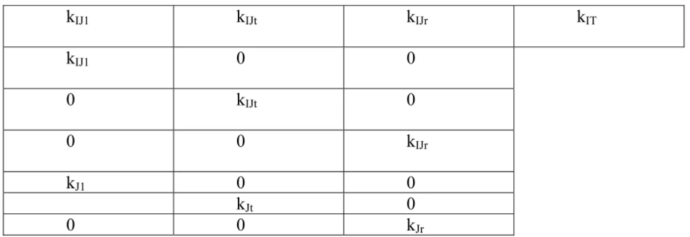
quoted above when T is put in supplementary columns. For instance the point i being an active element is the barycenter of the couples (i, t) for t belonging to T. Identically, the supplementary line point t is the barycenter of passive couples (i, t) for i belonging to I. The precedent set of possibilities is displayed in figure 1 which comes from [Caz04].
kIJ1 kIJt kIJr kIT kIJ1 0 0 0 kIJt 0 0 0 kIJr kJ1 0 0 kJt 0 0 0 kJr
Figure 1: CA of kIxJT with supplementary tables kIT, kITxJT and kTxJT. If in addition Jt =J, we
can also add the supplementary margin table of order 2 kIJ. It is also possible to analyze kIT
with the supplementary table kIxJT (interclass analysis).
With the partition of JT following the Jt, we can also perform the interclass analysis of kIxJT
(which is equivalent to the analysis of the table kIT), or its intra-class analysis. An example of
application is given in [Caz 94] or [Mor00].
We can also do MFA or apply STATIS method to table kIxJT, which are equivalent, when the
margins on I of the tables kIJt are proportional, to perform CA of the table produced by kIxJT
with an ad-hoc ponderation of each table kIJt. More details on these analyses are given in
[Caz04].
Other analyses are possible, in particular if r, the number of elements of T is not too big (r = 2 or 3). Thus, we can do conditional analysis, in doing CA of each table kIJt (the columns of the
table crossing I with JT-Jt being of course passive).
VI 2 Case where It = I and Jt = J are independent of t (ternary table kIJT).
VI 2.1 classical analysis
In this case, we have a table kIJT crossing I, J and T. We call respectively kIJ , kJT and kIT the
binary margin tables and kI, kJ, kT the first order margins of kIJT.
Then, we can perform the analysis of the table kIxJT suggested in paragraph VI 1, adding the
table kIJ, in addition to the supplementary tables already quoted, the representation of j being
Replacing I by J, and then I by T, we can do two other analyses analogous to the one detailed in the paragraph VI 1.
If I, J and T play a symmetric role, it is interesting to perform the analysis of the Burt table BBZZ crossing Z = I ∪ J ∪ T with itself, the non diagonal blocks corresponding to the binary margins of the table kIJT, while the diagonal blocks give the first order margins in their
diagonal and zeros otherwise.
Often I and J play a symmetric role contrary to T. This is in particular the case if T is the time. We can then do an analysis that preserves this symmetry by analyzing kIJ (interclass analysis)
and adding the tables kIxJT, kIT, kITxJ, kTJ as supplementary elements, kITxJ corresponding to the
table kIJT where the tables kIJt = kt are superimposed and kTJ the transposed second order
margin of kJT.
The two precedent analyses (analysis of BZZ and analysis of kIJ) have the disadvantage of
ignoring the interactions of an order above 2. VI 2.2 Deeper analysis: interactions study
When the sets I, J and T play a symmetric role, we can do 6 analyses starting from the considerations developed above:
a) The analysis of the 3 tables of binary margin (with the ad-hoc supplementary tables) that are indeed interclass analysis.
b) The analysis of the 3 tables crossing respectively one of the three sets with the product of the two others (with always ad-hoc supplementary tables including the two binary margin tables crossing the first set with each one of the two others).
To choose between the analyses to perform, Choulakian ([Cho88]) proposes to use the decomposition of the Φ2 of the frequency table fIJT associated to kIJT:
Φ2 (I, J, T) = Φ2 (I, J) + Φ2 (J, T) + Φ2 (I, T) + INT (I, J, T) (1)
Φ2 (I, J) (resp. Φ2 (J, T) ; Φ2 (I, T)) being the Φ2 (i.e. the total inertia in CA) of the binary margin table fIJ (resp. fJT ; fIT) associated to the table fIJT, Φ2 (I, J, T) being written, with
obvious notations:
Φ2 (I, J, T) = Σ {(fijt – fi.. f.j. f..t) 2 / (fi..f .j.f..t)| i∈ I, j ∈ J, t ∈ T} (2)
We recall that Φ2 (I, J) = Σ {(fij. – fi.. f.j.) 2 / (fi..f.j.)| i∈ I, j ∈ J}, Φ2 (J, T) and Φ2 (I, T)
being defined in an analogous way. The interaction term (of order 3) INT (I, J, T) which appears in the decomposition (1) comes from this decomposition and the definition (2) of Φ2(I, J, T). In function of the terms that are negligible in the precedent decomposition, Choulakian proposes the analysis or the analyses to perform.
If no term is negligible, Choulakian proposes a generalization of CA starting from a generalization of the reconstitution formula with an interaction term of third order. We can also use the log-linear model. Given the importance of this last model, and its links with CA, we will talk in more details about it in paragraph IX 2.
Other more specific analyses have been proposed in the literature (see for instance [Abd00], [Den00]) to take into account of the very particular structure of a ternary table: intraclass analysis, analysis bringing out the interactions, etc…
Indeed, for instance in the analysis of a table kIxJT crossing I with JT = JxT, there are two
partitions of JT (the one induced by J and the one induced by T). We have therefore two interclass analyses that correspond to CA of tables kIJ and kIT. We can therefore perform the
associated intraclass analysis, and this gives in total six possible intraclass analyses versus three interclass analyses.
We can also build in the analysis of kIxJT a residual table between kIxJT and the associated
table in absence of interaction between J and T (considering the profile columns table of kIxJT,
we can consider that we have a model of variance analysis of two factors with repetition, and that allows to easily compute the model without interaction and therefore the residual term corresponding to the interaction). The analysis of the residual table is equivalent to CA of the table where the general term is given (with obvious notations) by [Den00]:
kij. k.jt/ k.j. + ki.t k.jt/ k..t - kijt
In a deeper analysis of a table crossing the social origin (set I) with the sex (set J) and the type of study done (set T ={Law, Exact Sciences, Humanities, Medicine, etc.}) Carlier ([Car 01]) proposes a generalization of the TUCKALS3 algorithm due to Kroonenberg ([Kro83]) using diagonal metrics defined from the first order margins of the frequency table fIJT. More
precisely, ifX = xIJT and Y = yIJT are two vectors of RIJT with respectively the components xijt and yijt, the scalar product of these two vectors is defined by :
<X, Y> = ∑{fi..f .j.f..t xijt yijt | i ∈ I, j ∈ J, t ∈ T}
writing :
hijt = (fijt – fi.. f.j. f..t) / (fi..f .j.f..t) ,
the decomposition of order (P, Q, R) hijt* of hijt given by TUCKALS3 (decomposition that
Carlier calls 3 way correspondence analysis) is defined by: hijt = hijt* + eijt
with : hijt* = ∑{gpqr aip bjq ckr| p=1, P ; q=1, Q ; r =1, R}
and we obtain hijt* writing that the norm of the residual vector eIJT of components eijt is minimal under the orthogonally constraints: ∑{fi..aip aip’ | i ∈ I}= δpp’ = 1 if p=p’ and zero
otherwise. Identically: ∑{f.j.bjq bjq’| j ∈ J} = δqq’ and ∑{f..t ctr ctr’ | t ∈ T} = δrr’.
It is easy to see that Φ2(I, J, T) is nothing else than the square of the norm of the vector hIJT of components hijt. We have :
|| hIJT||2 = Φ2(I, J, T) = || hIJT*||2 +|| eIJT||2
In the particular case where fJT = fJ ⊗ fT (independence of the two last variables), Carlier has
shown that with one ad-hoc point at the beginning for the TUCKALS3 algorithm, the 3 way correspondence analysis is equivalent to CA of the table fIxJT.
VII Ascending hierarchical classification and correspondence analysis.
We will not talk here of the usual succession of CA and ascending hierarchical classification (AHC), that can be completed by the k-means method. We will talk about the link between the two methods, in a theoretical and practical point of view.
We first recall that when we have a contingence table kIJ partitioned in blocks (I = ∪ { Ib |
b=1, r }, J = ∪ { Jb | b=1, r }), where only the diagonal blocks are non null, AHC of one of
the two sets, I for instance, with the chi-2 metric and the aggregation criteria of inertia does not allow, except in very particular cases, to find the corresponding partition ([Rou89]). But we can (Corr Hier, [Ben73], tome 2, pp. 262-271) build a model showing a link between CA and AHC, model that has been generalized by Cazes ([Caz84]).
If we want to try to keep the symmetry between the two sets I and J, we can try to do a joint classification of these two sets. This is what has done Govaert ([Gov83]) with the algorithm CROKI2, but the joint classification that is done with a criteria of type dynamic clusters (or
k-means) does not drive to hierarchies of I and J but to partitions. Denimal ([Den07b]) performed an AHC of each set separately, with the chi-2 metric and an aggregation criteria with the same type as the one of VARCLUS, i.e. the minimization of the second (and smallest) eigenvalue of CA of the doubling table crossing the two aggregated classes. Then, he proposes to cut the two hierarchies HI and HJ built on I and J, taking into account of the
links between HI and HJ. Then, he gives some helps for interesting interpretations. In multiple
correspondence analysis, Denimal ([Den11]) proposes a joint classification of the set J of the modalities and of the set I of the observations of a complete disjunctive table kIJ adapting the
joint AHC of the set of the variables and the observations of a measures table ([Den07a]). In this case, we start to do AHC of the set J of the modalities and then AHC of I is built starting from the AHC obtained on J.
VIII Correspondence analysis and classical statistics
CA and more generally Data Analysis use classical statistics to validate results or to help interpretations. In particular, the chi-2 test can be used in CA of a contingence table to detect the number of retained factors. Identically, when we have an illustrative explicative variable x (therefore not having been used in the analysis), we can study its links with the factors coming from CA, and this allows to refine the interpretation. If x is quantitative, we can test if this variable is significatively correlated to a factor in computing the correlation between x and this factor and doing the Student test associated, or doing a non parametric test like the rank correlation test of Spearman. If x is qualitative, we can test if a factor can be considered as an interclass factor (i.e. linked to the partition structure defined by x) using an usual variance analysis test. We can also test for each modality of x if the mean of a factor on the individuals having taken this modality is significatively different of the general mean of this factor which is zero by construction.
The statistics associated to the precedent tests use the normality hypothesis. We can forget this hypothesis considering that these statistics are indicators which allow doing comparisons or classing in simple descriptive point of view.
We can also give up the normal hypothesis by using more general hypothesis ([Ler98]): frequency hypothesis, associated with the notion of ‘‘test value’’ (see for instance [Leb95]), combinatory hypothesis, based on permutation tests, and more generally, Bayesian hypothesis.
We can notice that the ‘‘test value’’ that, in the example of an illustrative modality, gives in a normalized way (going back to a centered reduced normal variable) the difference on a factorial axis between the mean of the absciss of the individuals having taken this modality and the general mean which is zero, is a very useful indicator which is provided by the software SPAD and which is also used to help the interpretation of a classification.
IX Correspondence analysis and modelling technique.
IX 1 The reconstitution formula considered as a modelling technique
The data reconstitution formula that allows the exact reconstruction of a frequency table fIJ
from the margins, the factors and the eigenvalues coming from CA of this table can be considered as a model when we approach the table with the r first factors.
This formula can be written, indicating by fij*the approximation of the general term fij of fIJ
when we keep r factors:
where ϕI
α = {ϕiα | i ∈ I } and ϕJα = {ϕjα | j ∈ J } are the factors on I and J with variance 1
associated to the eigenvalue λα and fI = {fi. | i ∈ I } and fJ = {f.j | j ∈ J } the margins of fIJ.
We can notice that near independence, the previous formula is very near of the log-linear model.
Indeed, (3) can be approximatively written doing a first order limited development: Log (fij*) = Log (fi.) + Log (f.j) + Σ {(λα) 1/2 ϕiα ϕjα | α= 1, r}
This corresponds to the log–linear model
Log (fij*) = μ + αi + βj + γij (4)
with μ = 0, αi = Log (fi.), βj = Log (f.j), and where the interaction term γij is of the form
Σ{(λα)1/2 ϕiα ϕjα | α= 1, r } , term that can be reduced if r = 1 to a multiplicative interaction
term (λ1)1/2 ϕi1 ϕj1. One can notice that the absence of interaction corresponds to the
independence, which makes that the log–linear model presents little interest when we have only 2 variables, except if modelling the interaction term.
We will give two examples of such modelling with only one keeped factor in the first one, and two in the second one.
If only one factor seems sufficient to explain the data and if the modalities of one or two variables that we cross to obtain the table fIJ are ordered, and if this order is respected (or
nearly respected) on the first factorial axis, we can do hypotheses of constant spacing between adjacent modalities on this axis. We can also suppose equal value for two near modalities on this axis (and therefore in space), which is equivalent to pool these modalities and therefore to cumulate the two lines or columns associated. Thus, one obtains a more sophisticated model (than the initial model of CA) where the parameters are estimated from CA under constraint, which is equivalent to a fit using the least squares method.
An example of such approach is given by Goodman [Goo85] to study the link between the mental state (4 modalities) and the socio-economical status of the parents (6 modalities), these two variables being measured on a sample of 1600 individuals. In the previous modelling, Goodman uses to estimate the parameters either the least squares method (which corresponds to CA), either the maximum likelihood method, and he proposes some tests to validate the proposed model. The data reconstitution formula corresponds to the RC association model of Goodman.
The second modelling example where two factors are used is given by Worsley ([Wor87]). The used table crosses a set J of 9 suicide modes with a set I product of the sex by the age cut in 17 classes, i.e. 34 modalities in total. The first factorial axis (52% of the inertia) opposes men and women, while the second axis (38% of the inertia) seems to show for each sex a linear effect of the age.
The formula (4), deduced from (3) with r = 2, can be put in the following form, by taking into account the precedent observations:
log (fij*) = μ + αi + βj + x1i u1j + x2i u2j
where x1i = 0 for a woman and 1 for a man, while x2i = k if i = 2k -1 or i = 2k, where 2k-1
IX 2 Correspondence analysis and log-linear model in the multiple table case
We only studied in § VI the case of the multiple tables of third order, but in practice, the number of variables is often greater.
The problem is then to detect the significant interactions between the variables. Indeed CA allows only detecting the second order interactions. We can always analyze interactions of greater order, in building the products of variables. Thus in a ternary table fIJT, CA of the table
fIxJT crossing I with T = J x T allows to study the third order interaction. Then, CA is made on
the table crossing the first variable with the product of the two others. There are three possibilities depending of the choice of the variable which is not in the product. The case is more complicated when we have 4 or more variables, the number of analyzable tables using all the variables for study the maximum order interaction, becoming quickly very high (three tables with 3 variables, as seen above, seven with 4, fifteen with 5, thirty-one with 6, etc...). Nevertheless, in the case of 4 variables Choulakian ([Cho88]) gives, like in the 3 variables case, some suggestions to analyze the ad-hoc tables, based on the decomposition of the Φ2 which the definition is analogous to the one given in § VI 2.2 in the 3 variables case.
It is then interesting to use the log-linear model to detect the significant interactions. The simultaneous use of CA and log-linear model can then be useful for the users, either doing CA of one or many tables suggested by the log-linear model, either doing a partial analysis taking into account some results of the log-linear model to eliminate, for instance, a very strong interaction and analyzing more in detail the data once this interaction has been eliminated (see § IV 2.2), or still deducting a log-linear model from results of a previous CA (see end of § IX 1).
The link between log-linear model and CA is studied in [Leb95] who gives a little bibliography on the subject with the book of Van der Heidjen ([Van87]) and the paper with discussion of Goodman ([Gou 91]) and also a certain number of papers published in the Revue de Statistique Appliquée (RSA) with in particular the special issue (number 2 of 1987) comparing French and Anglo-Saxon methodologies for the analysis of qualitative data.
We will just here recall one of the first articles published on this subject in RSA ([Dau80]). This paper studies the link between 6 variables, 5 variables with 2 modalities relative to the workmanship, and the region variable (the 21 French regions). Starting from a survey done on almost 20000 French farms, the authors do CA of the table of dimensions 32 (25) x 21 crossing the product of the binary variables with the region variable. This allows to interpret the axes 1 and 2 that represent the two third of the information but not the following axes. The study by the log-linear model of the interactions of order 2, 3 and 4 has allowed to complete and to refine the results obtained by CA.
To end, we point out the work of Kroonenberg and Anderson ([Kro06]) which compare additive modelling (with link to CA) and multiplicative modelling (with link with log-linear model and its extensions where interactions are bilinear modelling (RC association model)) to study three-way contingency tables.
IX 3 Correspondence analysis as an intermediate step in a modelling problem
Like any factorial analysis technique, CA acts as a data compression method before the modelling phase. Furthermore, the simultaneous use of CA and a model allows having two complementary views of the data, and this can allow refining the modelling.
We will only quote three examples of the common use of CA with other statistical methods in a modelling problem:
If we have the estimation of a probability law, for instance with an histogram, and if this law is a mixture of known probability laws (for instance, some Poisson’s laws with fixed parameters), the estimation of the unknown proportions pi (1 ≤ i ≤ k) can be done starting
from a regression under the constraint that the coefficients pi are positive or equal to zero, and
that their sum is equal to 1. The precedent problem being badly conditioned, the regression can be wrong, and this is why it is interesting to compress the data doing a regression (with constraint) on the first factors of CA of the table of the known probability laws ([Caz78]). A classical example, where CA is very often used, is the scoring, where we try to foreseen the class of an individual (good or bad payer; alive or deceased, etc…) as a function of explicative variables (qualitative and quantitative). After the division in classes of the numerical explicative variables and the construction of the complete disjunctive table kIJ of all
explicative variables, one proceeds to the discriminant factorial analysis on the factors coming from CA of this table, selecting the factors associated to a fixed inertia percentage (80 or 90%) and discriminating (we can test this by a classical variance test analysis). This is the DISQUAL method introduced by Saporta ([Sap77]).
On can also build the table kCJ crossing the set C of the two modalities of the variable to be
explained with the set J of all the explicative modalities, and do CA of this table which gives one single axis opposing the centers of gravity of the two classes to be foreseen. The projection on this axis, in supplementary elements, of the set I of the individuals, characterized by the explicative modalities, gives the score that allows affecting each individual to a class. This is the barycentric discriminant analysis (BDA; [Nak77]) that can easily be generalized, like DISQUAL, to the case where the variable to explain contains more than two modalities.
If, in the DISQUAL method, we keep all the factors, we obtain the same discriminant axis in the space RJ of the explicative modalities that in BDA, i.e. the axis joining the barycenter of
the two modalities to be foreseen. On the other hand, the discriminant scores are different, because in the first case, we project the individuals with the inertia metric, which corresponds to work (with the usual metric) on the factors on J of variance 1, while in the second case, we use the chi-2 metric coming from CA of kCJ (or kIJ), which is equivalent to work (with the
usual metric) on the usual factors, i.e. the factors of eigenvalue variance.
We can finally notice that instead of doing the factorial discriminant analysis, we can also proceed to the logistic regression on the factors coming from CA of the complete disjunctive table kIJ.
In the third example ([Mor94]), the simultaneous use of CA, AHC, PCA and of the Box-Jenkins method has allowed to foreseen the journal sale quantity of a certain number of wholesalers with a better accuracy than the one provided by the experts. The starting data is a table kIT crossing a set I of 1577 wholesalers with a set T of 157 weeks, the general term of
table of the table kIT followed by an AHC allows defining wholesaler classes. For each class,
we then proceed to PCA of the under-table of kIT corresponding, and the data reconstitution
formula allows to express the general term k(i, t) as a function of the average m(t) of the sales in the class and of the factors Fα (i) and Fα (t), the precision being sufficient if we keep the
two first factors. The modelling of m(t), F1 (t) and F2 (t) by a SARIMA process has allowed
to foreseen k (i, t) with a good precision, as said above. X Factorial analysis use in the work environment
In the French public sector, factorial analysis (CA, PCA) is mostly used in university’s laboratories (applied mathematic laboratories, psychology or sociology laboratories, etc...), in the applied mathematic departments of the public research organization (INRIA, INRETS, etc...) and in the engineer schools, in particular the agronomy schools.
If, in the private sector, PCA is the factorial technique that seems the more used, this is mostly multiple correspondence analysis (instead of the binary) that is used, either as an intermediate step in a prevision methodology (for instance the scoring), either to analyze a survey in a marketing or geo-marketing service, for instance.
Among the data analysis techniques the most used during their training course by the students of schools in statistics or of second degree master, we can quote the regression, the discriminant analysis, the logistic regression, the PLS regression and, more generally, the PLS approach (PLS Path Modelling), the PCA, the MFA, the classification methods, the neural networks, and in particular the Kohonen cards, etc… The PLS regression is being developed a lot since 15 years to study for instance data from near infra-red spectroscopy, this type of data appearing often in quality control and becoming numerous with the development of performing spectrometers. We can notice also that some extensions or interesting methodologies based on factorial analysis have been developed in the framework of the sensorial analysis which has taken a great importance since few years.
Nevertheless, it seems that in a general way, Data Analysis, and in particular the factorial methods remain still not enough used in France, while they could provide great help in numerous cases to users having data bases every day more important and complex.
Let me finally highlight the recent connexion between Data Analysis and Statistical Learning communities, connexion that led to the symposium SLDS (Statistical Learning and Data Sciences) 2009 in the Paris-Dauphine University in April 2009. The most important communications of this event have just been published in a special issue (number 42, summer 2010) of the review MODULAD.
XI Bibliography
[Abd00] ABDESSEMED, L., ESCOFIER, B. (2000) : Analyse de l’interaction et de la variabilité inter et intra dans un tableau de fréquence ternaire, in L’analyse des correspondances et les techniques connexes. Approches nouvelles pour l’analyse statistique des données, Eds. J. MOREAU, P.A. DOUDIN, P. CAZES, Springer, pp. 145- 164.
[Bas80] BASTIN, Ch., BENZECRI, J.P., BOURGARIT, Ch., CAZES, P. (1980) : Pratique de l’analyse des données, Tome 2 : Abrégé théorique. Etude de cas modèles, Dunod, 477 pages.
[Ben73] BENZECRI, J.P. (1973): L’analyse des données, Tome 1 : La taxinomie, 627 pages ; Tome 2 : L’analyse des correspondances, Dunod, 619 pages.
[Ben77] BENZECRI, J.P. (1977): Sur l’analyse des tableaux binaires associés à une correspondance multiple, [Bin Mult.], CAD, Vol. 2, n° 1, pp. 55, 71.
[Ben80] BENZECRI, J.P., BENZECRI, F. (1980) : Pratique de l’analyse des données, Tome 1 : Analyse des correspondances. Exposé élémentaire, Dunod, 432 pages.
[Ben81] BENZECRI, J.P. (1981) : Pratique de l’analyse des données, Tome 3 : Linguistique & lexicologie, Dunod, 575 pages.
[Ben82] BENZECRI, J.P. (1982) : Histoire et préhistoire de l’analyse des données, Dunod, 159 pages.
[Ben86] BENZECRI, J.P., BENZECRI, F. (1986) : Pratique de l’analyse des données, Tome 5 : Economie, Dunod, 543 pages.
[Ben92a] BENZECRI, J.P. (1992) : Correspondence Analysis Handbook, Dekker, 678 pages. [Ben92b] BENZECRI, J.P., BENZECRI, F., MAITI, G.D. (1992) : Pratique de l’analyse des données, Tome 4 : Médecine, pharmacologie physiologie clinique, Statmatic, 542 pages. [Car 01] CARLIER, A. (2001): Examples of 3-ways correspondence analysis (not published). [Caz78] CAZES, P. (1978) : Estimation de la statistique de multiplication du premier étage d’un photomultiplicateur à dynodes, [Photomultiplicateur], CAD, Vol.3, n° 4 pp. 393, 417. [Caz82] CAZES, P. (1982) : Note sur les éléments supplémentaires en analyse des correspondances, I : [El Sup.1], Pratique et utilisation, CAD, Vol.7, n° 1, pp. 9-23 ; II : [El Sup.2], Tableaux multiples, CAD, Vol.7, n° 2, pp. 133-154.
[Caz84] CAZES, P. (1984) : Correspondances hiérarchiques et ensembles associés, Cahiers du B.U.R.O., nos 43-44, pp. 43-142
[Caz90] CAZES, P. (1990) : Codage d’une variable continue en vue de l’analyse des correspondances, RSA, Vol. 38, n° 3, pp. 33-51.
[Caz91] CAZES, P., MOREAU, J. (1991): Analysis of a contingency table in which the rows and columns have a graph structure, in Symbolic-Numeric Data Analysis and Learning, Eds. E. DIDAY, Y. LECHEVALLIER, Nova Sciences Publishers, pp. 271-280.
[Caz94] CAZES, P., MOREAU, J., DOUDIN, P.A. (1994) : Etude des variabilités interindividuelles et intraindividuelles dans un questionnaire où toutes les questions ont le même nombre de modalités. Application à une recherche sur le développement de l’intelligence, RSA, Vol. 42, n° 2, pp. 5-25.
[Caz04] CAZES, P. (2004) : Quelques méthodes d’analyse factorielle d’une série de tableaux de données, la revue de MODULAD, n° 31, pp. 1-31.
[Che93] CHESSEL, D., MERCIER, P. (1993) : Couplage de triplets statistiques et liaisons espèces – environnement, Eds. LEBRETON, J.D., ASSELAIN, B., Masson, Paris, pp. 15-44. [Cho88] CHOULAKIAN, V. (1988) : Analyse factorielle des correspondances de tableaux multiples, RSA, Vol. 36, n° 4, pp. 33-42.
[Dau80] DAUDIN, J.J., TRECOURT, P. (1980) : Analyse factorielle des correspondances et modèle log- linéaire : Comparaison des deux méthodes sur un exemple, RSA, Vol.28, n° 1, pp. 5-24.
[Den00] DENIMAL, J.J. (2000) : L’analyse factorielle des interactions, in L’analyse des correspondances et les techniques connexes. Approches nouvelles pour l’analyse statistique des données, Eds. J. MOREAU, P.A. DOUDIN, P. CAZES, Springer, pp. 165- 180.
[Den07a] DENIMAL, J.J. (2007a) : Classification factorielle hiérarchique optimisée d’un tableau de mesures, JSFdS - RSA, Vol. 148 n° 2, pp. 29, 63.
[Den07b] DENIMAL, J.J. (2007b) : Classification factorielle hiérarchique optimisée des lignes et des colonnes d’un tableau de contingence, JSFdS - RSA, Vol. 148 n° 3, pp. 37, 70. [Den11] DENIMAL, J.J. (2011): Extension aux correspondances multiples de la classification hiérarchique optimisée, JSFdS, à paraître.
[Esc79] ESCOFIER, B. (1979) : Traitement simultané de variables qualitatives et quantitatives en analyse factorielle, [Qualitatives et Quantitatives], CAD, Vol. 4 n° 2, pp. 137-146.
[Esc84] ESCOFIER, B. (1984) : Analyse factorielle en référence à un modèle. Application à l’analyse de tableaux d’échanges, RSA, Vol. 32 n° 4, pp. 25-36.
[Esc98] ESCOFIER, B., PAGES, J. (1998) : Analyses factorielles simples et multiples. Objectifs, méthodes et interprétation, 3éme éd., Dunod, 300 pages.
[Goo85] GOODMAN, L.A. (1985) : Correspondence analysis models, log-linear models, and log-bilinear models for the analysis of contingency tables, Proceedings of the 45th session of ISI, Amsterdam.
[Goo91] GOODMAN, L.A. (1991): Measures, models, and graphical displays in the analysis of cross-classified data (with discussion), J. of Amer. Stat. Assoc., vol.86, pp.1085-1138. [Gov83] GOVAERT, G. (1983) : Classification croisée, thèse d’état, Un. Paris 6.
[Kro83] KROONEMBERG, P.M. (1983): Three-mode principal component analysis: Theory and applications, Leiden, DSWO Press.
[Kro06] KROONEMBERG, P.M., ANDERSON, C.A. (2006): Additive and multiplicative models for three-way contingency tables: Darroch (1974) revisited, in Multiple Correspondence Analysis and Related Methods, Ed. M. GREENACRE and J. BLASIUS, Chapman & Hall, Ch. 21, pp. 455, 486.
[Leb71] LEBART, L. (1971) : Note sur l’analyse des correspondances n-aires (not published). [Leb95] LEBART, L., MORINEAU, A., PIRON, M. (1995) : Statistique exploratoire multidimensionnelle, Dunod, 456 pages.
[Leb06] LEBART, L. (2006) : Validation Techniques in Multiple Correspondence Analysis, in Correspondence Analysis and Related Methods, Ed. M. GREENACRE and J. BLASIUS, Chapman & Hall, Ch.7, pp.179, 195.
[Ler98] LEROUX, B. (1998) : Inférence combinatoire en analyse géométrique des données, Math. Inf. Sci. Hum., Vol. 36, numéro 144, pp. 5-14.
[Mor00] MOREAU, J., DOUDIN, P.A., CAZES, P. (2000) : Etude de la variabilité intraindividuelle par l’analyse des correspondances, in L’analyse des correspondances et les techniques connexes. Approches nouvelles pour l’analyse statistique des données, Eds. J. MOREAU, P.A. DOUDIN, P. CAZES, Springer, pp. 106- 119.
[Mor94] MORINEAU, A., SAMMARTINO, A.E., GETTLER-SUMMA, M., PARDOUX, C. (1994) : Analyse des données et modélisation des séries temporelles. Application à la vente de périodiques, RSA, Vol. 42, n° 4, pp. 61-81.
[Nak77] NAKACHE, J.P., LORENTE, P., BENZECRI, J.P., CHASTANG, J.F. (1977) : Aspects pronostiques et thérapeutiques de l’infarctus myocardique aigu compliqué d’une défaillance sévère de la pompe cardiaque. Application des méthodes de discrimination, [Aorte], CAD, Vol.2, n° 4, pp. 415-434.
[Rou89] ROUSSEAU, R. (1989) : Reconnaissance de la structure de blocs d’un tableau de correspondance par la classification hiérarchique (suite), [Rec.Bloc.II], CAD, Vol 14, n° 3, pp. 257-266.
[Sap77] SAPORTA, G. (1977) : Une méthode et un programme d’analyse discriminante sur variables qualitatives, Premières Journées Internationales, Analyse des Données et Informatique, INRIA, Versailles.
[Tuc58] TUCKER, L.R. (1958): An inter-battery method of factor analysis, Psychometrica, Vol. 23, n° 2, pp. 111-136.
[Van 87] VAN DER HEIDJEN, P.G.M. (1987): Correspondence analysis of longitudinal categorical data, DSWO Press, Leiden, 282 pages.
[Wor87] WORSLEY (1987) : Un exemple d’identification d’un modèle log- linéaire grâce à une analyse des correspondances, RSA, Vol. 35, n° 3, pp. 13-20.
[Yag77] YAGOLNITZER (1977) : Comparaison de deux correspondances entre les mêmes ensembles, [Compar. Corr.], CAD, Vol. 2, n° 3, pp. 251, 264.