Red State, Blue State: Examining Federal Transfers to the States, 1983-2004

(1)

Summary:

This report seeks to explain the transfer of United States federal funds to the states by examining the political and economic motivators in certain federal spending categories, including total expenditures, defense expenditures, procurement contracts, grants awarded, loan and insurance spending, and the net tax burden (variable not yet fully calculated). This report updates previous research in federal transfers, using twenty-two years (1983-2004) of electoral, population, spending, taxation and state economic data for the states. Using panel data methodology in STATA, various political and economic variables are examined for their impact on this era of neo-conservative resurgence in the United States, particularly interaction variables that highlight political party alignment between the executive branches of federal and state government, alignment with the majority controlling parties in the legislative branch and various interaction and political party variables.

(2)

Table of Contents

Summary i

Table of Contents ii

List of Graphs and Tables iii

Introduction 1

Section I

- Review of Existing Literature 3

- Modeling Transfers to the States 9

Section II

- Data Selection 11

- Summary of Variables Used in Analysis 12 Section III

- Empirical Results and Analysis 18

- Summary of Empirical Results 43

- Political Analysis 45

Conclusion 51

(3)

List of Graphs, Models and Tables

Table 1: Summary of Relevant Research p.7

Table 2: Summary Definitions of Dependent Variables p.12 Table 3: Statistical Summary of Dependent Variables p.13 Table 4: Summary Definitions of Independent Variables p.13 Table 5: Statistical Summary of Independent Variables p.14

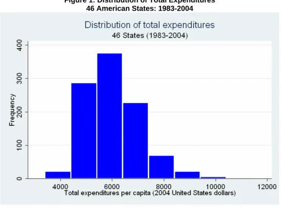
Figure 1: Distribution of Total Expenditures p.16

Figure 2: Distribution of Defense Expenditures p.16

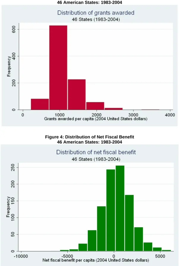
Figure 3: Distribution of Grants Awarded p.17

Figure 4: Distribution of Net Fiscal Benefit p.17

Model 1.1: Total Expenditures (majority alignment) p.18 Model 2.1: Defense Expenditures (majority alignment) p.20

Model 3.1: Grants Awarded (majority alignment) p.22

Model 4.1: Total Procurement (majority alignment) p.23 Model 5.1: Defense Procurement (majority alignment) p.25 Model 6.1: Other Procurement (majority alignment) p.26 Model 7.1: Retirement and Disability (majority alignment) p.27

Model 8.1: Other Payments (majority alignment) p.28

Model 1.2: Total Expenditures (pure party alignment) p.29 Model 2.2: Defense Expenditures (pure party alignment) p.31 Model 3.2: Grants Awarded (pure party alignment) p.32 Model 4.2: Total Procurement (pure party alignment) p.34 Model 5.2: Defense Procurement (pure party alignment) p.35 Model 6.2: Other Procurement (pure party alignment) p.37 Model 7.2: Retirement and Disability (pure party alignment) p.38 Model 8.2: Other Payments (pure party alignment) p.39

Model 9.1: Net Fiscal Benefit p.41

Model 9.2: Net Fiscal Benefit p.42

Table 6: Summary of Majority Alignment Model Results p.43 Table 7: Summary of Political Party Alignment Model Results p.44

(4)

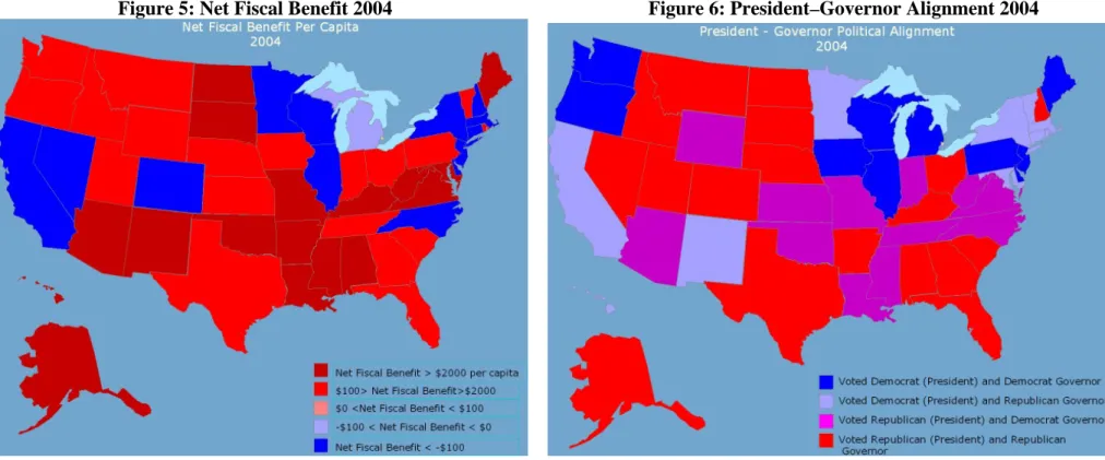
Figure 5: Net Fiscal Benefit 2004 p.48

Figure 6: President-Governor Alignment 2004 p.48

Figure 8: President-Governor Alignment 1994 p.49

(5)

Introduction:

Following the 2004 presidential elections, red and blue colored maps circulated, dividing the United States into two colors by electoral vote allocated to the presidential

candidates—typically red for the Republican electoral votes and blue for Democratic electoral votes. A preponderance of these maps attempted to explain many economic, social and political factors along this red-blue divide.

A graphic of particular interest is one that shows the “blue states”—the states that voted the Democratic ticket in 2004 as the “losers” in federal funding received, while the “red states”—the states that voted the Republican ticket are the “winners,” receiving far more federal aid than the blue states in per capita and net transfer terms. Paradoxically, the “red state" values of self-reliance, free markets, small government and fiscal restraint put the American conservatives in power, and returned George W. Bush and the Republican congressional majority to power in 2004. This paper will take a recent historical perspective in examining federal transfers to the states and its political-economic components

Intergovernmental transfers and equity are a perpetual bone of contention amongst the Canadian provinces and between them and the federal government. Accordingly, there is a wealth of information and scholarly study on fiscal federalism in Canada. In the United States, however, there are few rigorously explained political-economic models that examine federal transfers to the states, taking into account explicit transfers by category, such as block grants and spending programs, as well the net fiscal benefit. The net fiscal benefit (NFB) is defined as the amount of public services received minus the amount of taxes paid. In this paper, the net fiscal benefit will be calculated for each state.

To test whether there is a political-economic rationale for the allocation of federal funds, this report will model the transfers from the federal government to the states in per capita and net transfer terms as dependent variables. Independent variables that will be

(6)

population of the states, Electoral College representation and votes for the past twenty-two years, federal Congressional representation, state gubernatorial representation and state legislative representation.

(7)

Section I: Literature Review and Analytical Framework

Review of Existing Literature:

A partisan theory of federal budget allocation is a far from recent phenomenon and empirical studies abound in the literature. The majority of existing lworks focuses on the powers of the legislative branch of government at the federal level, particularly the impact of committee membership and that of individually powerful members of

Congress. Studies on the impact of the president date back, in large part, to the New Deal presidency of Franklin D. Roosevelt.

However there are a few recent studies on the impact of the president in budget

allocation, as well as annual studies of the federal budget and the States, a joint project between the Taubman Center for State and Local Government at the Kennedy School of Government at Harvard University and Senator Daniel Patrick Moynihan (Democrat of New York, 1976-2000). This report is then descriptive by nature, comparing the different states in the five major areas of expenditure defense, non-defense discretionary, Social Security, Medicare, and assistance programs. Following the death of Senator Moynihan, a similar report has not been published, although there is supposedly a report for 2003 in progress1.

A review of recent literature has both provided inspiration and guidance to our report. Some important literature includes:

Slicing the Federal Government Net Spending Pie: Who Wins, Who Loses and Why Cary Atlas, Thomas Gilligan, Robert Hendershott and Mark Zupan (1995)

The authors examine the distribution of federal net spending, defined as taxes minus expenditures, across the fifty states from 1972 to 1990. The authors limit the scope of their inquiry to the legislative branch, and advance the hypothesis of an

1_{Home page of lead report author, Herman B. “Dutch” Leonard shows the 2003 report as “in progress”:} http://dor.hbs.edu/fi_redirect.jhtml?facInfo=pub&facEmId=hleonard

(8)

“overrepresentation bias” that gives preference to small states. The paper examines the effect of this “overrepresentation bias,” and pays particular attention to the Senate, where a populous state such as California receives the same treatment as the far less populous Delaware. This paper was one of the first to account for this type of bias, and is often cited in subsequent literature.

Allocating the U.S. Federal Budget to the States: The Impact of the President Valentino Larcinese, Leonzio Rizzo and Cecilia Testa (2006)

The paper provides empirical evidence on the determinants of the U.S. federal budget allocation to the states. Expanding and departing from existing literature that gives prominence to Congress and to vote-purchasing behavior with swing states and strongly supportive states, the authors conducted an empirical investigation on the impact of presidents during the period 1982–2000. This study takes the entire federal expenditure budget as the dependent variable. There are several separate hypothesis tested, with respect to presidential politics. States that heavily supported the incumbent president in past presidential elections tend to receive more funds, while marginal and swing states are not rewarded. Party affiliation is examined to the extent that the governor (state level executive branch) party affiliation is the same as the president. Larcinese et al find that states in which the executive branch party (the party of the governor) is aligned with the president’s political party receive more federal funds, while states opposing the

president’s party in Congressional elections are penalized. They posit their results as evidence for presidential engagement in tactical distribution of federal funds and also as support for partisan theories of budget allocation.

There are several weaknesses to this approach, in that allocation of the federal budget is such that there is great flexibility in some categories of spending, whereas other

categories are severely restricted by demographics, such as is the case with Medicare, a federal health-care program universally applied to all Americans over the age of 65 eligible for Social Security payments. Medicare is one of the largest single-category federal transfers to the states, and the transfer is calculated using a universal formula that is functionally immune from major, pork-barrel type politically-biased manipulations.

(9)

Conversely, there are certain spending categories in which different branches of the government have more leeway. For example, the president, as the head of the U.S. Military has some discretionary impact in defense spending.

The Impact of Federal Spending on House Election Outcomes Steven Levitt and James M. Snyder (1997)

The paper examines vote-purchasing behavior in the House of Representatives, to the extent that incumbent members of Congress are rewarded (by re-election) for bringing federal dollars into their district. Using an instrumental variables model, Levitt and Snyder account for the omitted variable bias engendered by the potential variation in effort of representatives up for re-election. Incumbents expecting difficulty are expected to behave differently than those who do not, and thus may perhaps work harder to bring federal dollars to their district. Unfortunately, the time period covered in this paper is limited in scope to the eight years (1983-1990) covered by the Federal Assistance

Awards Data System (FAADS), as this data set contained annual district-level outlays on a programmatic basis, totaling over half of the federal budget. Most importantly, the paper makes the distinction between high and low-variation programs, the high variation programs being more discretionary in nature and thus more amenable to political

manipulation rather than direct entitlement programs, such as social security and

Medicare. Nonetheless, the empirical evidence produced from this paper differs than that from previous studies, in that they find evidence that an increase in federal spending benefits congressional incumbents, “purchasing” as much as 2% of the popular vote with an additional $100 in per capita spending.

The Determinants of Success of Special Interest in Redistributive Politics Avinash Dixit and John Londregan (1996)

Economic redistribution occurs on two levels in the political process, the first on a grand scale reflecting the economic beliefs of a country, and is achieved through taxation and social spending. On a secondary level, economic redistribution can occur more tactically, and can coincide with the grander scheme of redistribution, and can take on a variety of forms including subsidies, tax expenditures, public works projects and other schemes that

(10)

are often labeled as “pork barrel.” This theoretical paper examines the determinants of whether a heterogeneous interest group will receive favors in pork-barrel politics, where there is majority voting in a two-party system. Individuals must choose between party affinity and their own transfer receipts. The results of this model can yield two different outcomes as special cases, which are the competing theories of the “swing voter” and “machine politics.” In the swing voter outcome, both parties are equally effective at delivering transfers and thus attempt to capture the middle, politically centrist ground through economic favors. The machine politics outcome is achieved if each party is more effective in delivering favors to its own support group, thus leading the political parties to reward its core supporters.

These results can be extrapolated on an aggregate level, as these results can be applied to groups of people at the state level, yielding either favors for swing states or rewarding those states that are stalwarts of either party. They suggest that that many economically inefficient policies with unequal allocation across a society fit well within this model of redistributive politics, that is, programs with a high potential for variance and unequal spending are often exploited to favor certain political outcomes in a two-party electoral system.

(11)

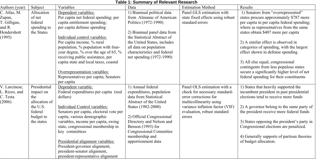
Table 1: Summary of Relevant Research

Authors (year) Subject Variables Data Estimation Method Results

C. Atlas, M. Zupan, T. Gilligan, and R. Hendershott (1995) Allocation of net federal spending to the States Dependent variables:

Per capita net federal spending; per capita entitlement spending; per capita defense spending Individual control variables: Per capita income, % rural

population, % population with four-year degree, % over the age of 65, % receiving public assistance, per capita state and local taxes, coastal Overrepresentation variables: Representatives per capita; Senators per capita

1) Biannual political data from Almanac of American Politics (1972-1990) 2) Biannual panel data from the Statistical Abstract of the United States, includes all data on population characteristics and federal net spending (1972-1990)

Panel GLS estimation with state fixed effects using robust standard errors

1) Senators from “overrepresented” states procure approximately $787 more per capita in per capita federal spending; where as representatives from the same states obtain $407 more per capita

2) A similar effect is observed in categories of spending, with the largest effect shown in defense spending 3) All else equal, congressional contingents from less populous states secure a significantly higher level of net federal spending for their constituents V. Larcinese, L. Rizzo, and C. Testa (2006) Presidential impact on the allocation of the U.S. federal budget to the states Dependent variable:

Federal expenditures per capita (real dollars)

Individual Control variables:

Senators per capita, electoral vote per capita, various demographic

variables, income per capita, swing state, congressional membership in key committees

Presidential alignment variables: President-governor alignment, president-senator alignment, president-representative alignment

1) Annual federal expenditures, population data from Statistical Abstract of the United States (1982-2000) 2) Official Congressional Directory and Nelson and Benson (1993) for Congressional Committee membership and

apportionment data

Panel OLS estimation with a check for necessary standard-error corrections for

multicollinearity using variance inflation factor (VIF) evaluation, robust standard errors

1) States that heavily supported the incumbent president in past presidential elections tend to receive more funds 2) A governor belong to the same party of the president receive more federal funds 3) States opposing the president’s party in Congressional elections are penalized. 4) Generally supports of partisan theories of budget allocation.

(12)

Authors (year) Subject Variables Data Estimation Method Results S. Levitt, J.

Snyder (1997) Impact of federal spending on House election outcomes

Dependent variable:

Per capita federal spending (in various categories) to a district Control variables:

Population characteristics, share of democratic vote, share of republican vote, % share in state per capita income, incumbency, closeness to the state’s capitol city

Instrumental variable:

In-state out-of-congressional district spending

1) District-level outlays of spending from 1983-1990 from Bickers-Stein Federal Awards Assistance Data System, demographic and economic variables also from this data set

2SLS methods using in-state out-of-district spending as instrumental variable to solve the omitted variables problem of “effort” exerted by the incumbent to retain his or her seat, OLS used as baseline for comparison

1) Instrumental variable approach yields coefficients that are five times larger than the OLS estimate

2) Need to differentiate between different types of expenditures, namely high-variation and low-high-variation programs 3) Evidence of vote-purchasing behavior: an increase of $100 in per-capita

spending shows a 2% increase in the incumbent’s share of the popular vote B. Schor (2005) Determinants

of defense budget allocation

Dependent variable:

Per capita federal defense spending (logarithmic form) to a district Control variables:

Population characteristics, share of democratic vote, share of republican vote, income per capita, district voting patterns during presidential election years

1) District-level outlays of spending from 1983-1992 using the Consolidated Federal Funds Report 2) Current population survey (CPS) for demographic variables 3) Congressional Quarterly for presidential vote totals 4) Bureau of Economic Analysis for income totals

Bayesian multilevel modeling using Markov Chain Monte Carlo simulations; rejects panel regressions using corrected standard errors

1) No support for effective “targeting” of home states by House legislators. 2) Delegations dominated by Democrats unable to deliver more to their states (Democrats were controlling party of House during entire time period)

3) Highlights need to include predictors at different levels of analysis (e.g. federal, state, and interaction variables); previous literature assumes only local district level effects

(13)

Modeling Federal Transfers to the States:

The proposed economic models are:

Federal Expendituresstc= αt + βXst + δYst + θZst

Net fiscal benefitstc= αt + βXst + δYst + θZst

The dependent variable is expressed in total dollar terms. X is a vector representing demographic and economic data, Z is a vector representing political-institutional variables, and Y is an instrumental variable (when necessary) to correct for the well-documented overrepresentation bias, as well other measures to better document the effect of representatives in their district. The subscript “s” denotes the state, “t” the year, and “c” the category of expenditure or the net fiscal benefit. Regressions use random-effects GLS methods for panel data with STATA 9.0, using instrumental variables wherever necessary.

Three hypotheses are tested. The first two hypotheses correspond to federal spending categories (per the Consolidated Federal Funds Report) and the final hypothesis corresponds to the allocation of the net fiscal benefit.

H1: Political alignment by various combinations of actors on the federal level and between the federal and state level is important (alignment with majority party) for certain federal spending categories.

To test this hypothesis, the following model is proposed:

Expenditure categoryst = populationst + per capita tax burdenst + gross state product per

capitast + gross state product per capitast-1 + electoral vote per capitast + voted for

sitting presidentst + President-Governor alignmentst + Senate majority alignmentst +

(14)

H2: Pure party affiliation on federal and state levels is an important determinant for certain federal spending categories.

The hypothesis is tested using the model:

Expenditure categoryst = populationst + per capita tax burdenst + gross state product per

capitast + gross state product per capitast-1 + electoral vote per capitast + voted for

Republican President in officest + voted for Democrat President in officest + Republican

Governorst + Democrat Governorst + both Senators Republicanst + both Senators

Democratsst + majority of Representatives Republicanst + majority of Representatives

Democratst + State Senate majority Republicanst + State Senate majority Democratst +

State House majority Republicanst + State House majority Democratst

H3: The net fiscal benefit per capita can be allocated according to a majority alignment model or political party alignment model.

The hypothesis is tested using the following model:

Net fiscal benefitst = electoral vote per capitast + gross state product per capitast + gross

state product per capitast-1 + gross state product per capitast-2 + gross state product per

capitast-3 + gross state product per capitast-4 + gross state product per capitast-5 + gross

state product per capitast-6 + voted for sitting presidentst + President-Governor

alignmentst + Senate majority alignmentst + House majority alignmentst +

(15)

Section II

Data Selection:

The database used for the study draws from several sources, and is both political and economic in nature. Political data includes real changes observed every two years, with some categories exhibiting more variation than others. The presidential vote data includes the Electoral College vote apportionment and allocation by party, while the federal legislative branch includes apportionment data as it affects the House of Representatives. Changes in apportionment are made following the decennial census, and thus are applied for elections in 1982, 1992, and 2002, resulting in electoral office change early in the following year (1983, 1993, and 2003). These changes reflect real population and demographic shifts among the states, which shifts the allocation of four hundred and five representatives amongst the fifty states and disperses five hundred and thirty-eight electoral votes among the states and the District of Columbia. Each member of the House of Representatives serves a two year term and may be re-elected an unlimited number of times. Senators serve for staggered six-year terms so that elections are held for approximately one-third of the seats every other year; there are no term limits. On the state level, term limits, length of term and internal apportionment varies widely for the state level congress, as does the quantity of senators and representatives within each state. To facilitate comparison, the state-level congresses are assigned binary variables that represent the majority party within the State Senate and the State House of

Representatives. This data was obtained from the United States Congressional Almanac and the Book of the States.

The economic data includes federal transfers to the states, organized by major spending category. This paper makes use of the Consolidated Federal Funds Report (CFFR), annually published by the U.S. Department of the Census. This document aggregates the federal government expenditures or obligations in state, county, and sub-county areas of the United States (including the District of Columbia and U.S. Outlying Areas). The CFFR contains statistics on the geographic distribution of federal program expenditures

(16)

and obligations, using data submitted by federal departments and agencies. The CFFR expenditure data is “much more comprehensive than the much more commonly used Bickers-Stein Federal Awards Assistance Data (Shor 2005),” which was used in Atlas et al and Levitt and Snyder, 1995 and 1997. The population data is data from the official U.S. Census (for 1990 and 2000) and estimates for all other years. The state federal tax burden data is collected from the Tax Foundation and the U.S. Bureau of Economic Analysis. Gross state product (GSP), a measure of each state’s economic output in current dollars, is obtained from the Bureau of Economic Analysis.

Twenty-two years of data, from 1983 to 2004, is organized in yearly panels for forty-six states, excluding the District of Columbia, Hawaii and Alaska—following a well

established precedent in the literature. The states of Virginia and Maryland were also excluded from analysis. As the federal expenditure data is allocated by place of performance, including Virginia and Maryland could obscure political determinants in the allocation of federal funds.

Summary of Variables Used in Analysis:

Dependent Variables:

The definition and source of the dependent variables for all hypotheses are summarized in the following table.

Table 2: Summary Definitions of Dependent Variables

Variable Definition Source

Total Expenditures

all government spending and obligations, excluding contingent liabilities (total dollars)

Consolidated Federal Funds Report (CFFR)

Defense Expenditures expenditures for all Department of Defense agencies (total dollars) CFFR

Grants Awarded

all project-specific grants, all formula grants prescribed by law (total

dollars) CFFR

Total Procurement

Value of obligations for contract actions accorded to the place of

performance (total dollars) CFFR

Defense Procurement

Value of obligations for defense-related contract actions accorded

to the place of performance (total dollars) CFFR

Other Procurement

Value of obligations for nondefense-related contract actions

accorded to the place of performance (total dollars) CFFR Retirement and

Disability

all Social Security payments and federal employee retirement and

(17)

Other Payments

Other direct payments to individuals other than retirement and

disability, direct payments not for individuals (total dollars) CFFR

Net Fiscal Benefit

amount of public services received minus the amount of taxes paid (total dollars)

CFFR, Tax foundation, Book of the States

Alternatively, total expenditures can be defined as:

Total expenditures = defense expenditures + grants awarded + other procurement + retirement and disability + other payments

Defense expenditures include defense procurement; while total procurement is composed of defense and non-defense related federal procurement dollars.

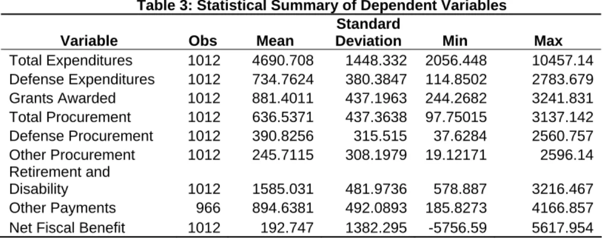
The statistical properties of the dependent variables, in total actual dollar terms per capita, are summarized in Table 3.

Table 3: Statistical Summary of Dependent Variables

Variable Obs Mean

Standard

Deviation Min Max

Total Expenditures 1012 4690.708 1448.332 2056.448 10457.14 Defense Expenditures 1012 734.7624 380.3847 114.8502 2783.679 Grants Awarded 1012 881.4011 437.1963 244.2682 3241.831 Total Procurement 1012 636.5371 437.3638 97.75015 3137.142 Defense Procurement 1012 390.8256 315.515 37.6284 2560.757 Other Procurement 1012 245.7115 308.1979 19.12171 2596.14 Retirement and Disability 1012 1585.031 481.9736 578.887 3216.467 Other Payments 966 894.6381 492.0893 185.8273 4166.857 Net Fiscal Benefit 1012 192.747 1382.295 -5756.59 5617.954

Independent Variables:

The independent variables are defined in the following table:

Table 4: Summary Definitions of Independent Variables

Variable Definition Source

Population United States resident population

United States Bureau of the Census

Population2 Square of population

Tax burden per capita

Average federal taxes paid, per capita, expressed in current dollars; includes accounting for the federal deficit as well as all federal

taxes including social insurance, excise, income and corporate Tax Foundation Income per capita Average income, per capita of a state's residents

United States Bureau of Economic Analysis

(18)

Electoral vote per capita

Electoral votes of a state divided by population, the votes are equal to a state's total number of representatives in congress (House plus Senate)

The Book of the States, United States Bureau of the Census

Senators per capita Number of senators (2) divided by population

GSP per capita Gross state product, expressed in per capita terms

United States Bureau of Economic Analysis Voted for sitting

president

Binary variable that takes value of 1 if state voted for sitting

president The Book of the States

President-governor alignment

Binary variable that takes value of 1 if president and governor are of

the same political party The Book of the States

Senate majority alignment

Binary variable that takes value of 1 if both senators from a state

are aligned with the majority party The Book of the States House majority

alignment

Binary variable that takes value of 1 if 50%+1 representatives from

a state are aligned with the majority party The Book of the States President-State

Congress majority alignment

Binary variable that takes value of 1 if president and the majority

party of a State's Congress are of the same political party The Book of the States Voted for Republican

sitting president

Binary variable that takes value of 1 if state voted for a Republican

sitting president The Book of the States

Voted for Democrat sitting president

Binary variable that takes value of 1 if state voted for a Democrat

sitting president The Book of the States

Republican governor

Binary variable that takes value of 1 if state's governor is

Republican The Book of the States

Democrat governor Binary variable that takes value of 1 if state's governor is Democrat The Book of the States Senators both

Republican

are Republican The Book of the States

Senators both Democrat

are Democrat The Book of the States

Representatives majority Republican

Binary variable that takes value of 1 if most representatives from a

state are Republican The Book of the States

Representatives majority Democrat

Binary variable that takes value of 1 if most representatives from a

state are Democrat The Book of the States

State Senate majority Republican

Binary variable that takes value of 1 if State Senate is majority

State Senate majority Democrat

Binary variable that takes value of 1 if State Senate is majority

Democrat The Book of the States

State House majority Republican

Binary variable that takes value of 1 if State House is majority

State House majority Democrat

Binary variable that takes value of 1 if State House is majority

Democrat The Book of the States

Coastal

Binary variable that takes value of 1 if State is on coastline (Gulf of Mexico, Pacific Ocean, Atlantic Ocean)

Map of the United States

Swing State

Binary variable that takes value of 1 if State voted within 5% of the winning margin in last presidential election

Atlas of U.S.

(19)

A summary of the statistical properties of each independent variable follows below:

Table 5: Statistical Summary of Independent Variables

Variable Obs Mean Std. Dev. Min Max

Tax Burden per capita ($US) 1012 4497.961 1629.382 1578.888 11512.43 Income per capita ($US) 1012 21280.19 6736.325 8576 45412 GSP per capita ($US) 1012 25408.74 8325.259 10114.91 63004.4

Voted for sitting president 1012 0.7371542 0.440397 0 1

President-governor alignment 1012 0.3320158 0.4711695 0 1

Senate majority alignment 1012 0.3300395 0.4704595 0 1

House majority alignment 1012 0.5592885 0.4967179 0 1

President-State Congress majority

alignment 1012 0.2183794 0.4133506 0 1

Population density (pop per square mile) 1012 143.5828 189.9263 4.635149 995.7769 Electoral vote per capita 1012 2.69E-06 1.05E-06 1.39E-06 6.62E-06 Senators per capita 1012 9.75E-07 9.89E-07 5.58E-08 4.41E-06

Population 1012 5325959 5776611 453401 3.58E+07

Population squared 1012 6.17E+13 1.55E+14 2.06E+11 1.28E+15 Voted for Republican sitting president 1012 0.5335968 0.4991166 0 1 Voted for Democrat sitting president 1012 0.2035573 0.4028425 0 1

Republican governor 1012 0.5158103 0.4999971 0 1

Democrat governor 1012 0.4703557 0.4993672 0 1

Senators both Republican 1012 0.2885375 0.4533064 0 1

Senators both Democrat 1012 0.2924901 0.4551311 0 1

Representatives majority Republican 1012 0.3695652 0.4829257 0 1 Representatives majority Democrat 1012 0.4841897 0.4999971 0 1 State Senate majority Republican 1012 0.4011858 0.4903808 0 1 State Senate majority Democrat 1012 0.5533597 0.4973904 0 1 State House majority Republican 1012 0.3695652 0.4829257 0 1 State House majority Democrat 1012 0.5948617 0.4911615 0 1

Swing State 1012 0.1976285 0.3984072 0 1

Coastal state 1012 0.3685771 0.4826574 0 1

The following graphics show the frequency and distribution of four key dependent variables in per capita terms: total expenditures, defense expenditures, grants awarded and the net fiscal benefit.

(20)

Figure 1: Distribution of Total Expenditures 46 American States: 1983-2004

Figure 2: Distribution of Defense Expenditures 46 American States: 1983-2004

(21)

Figure 3: Distribution of Grants Awarded 46 American States: 1983-2004

Figure 4: Distribution of Net Fiscal Benefit 46 American States: 1983-2004

(22)

Section III

Empirical Results:

Hypothesis 1: Political alignment by various combinations of actors on the federal level and between the federal and state level is important (alignment with majority party) for certain federal spending categories

In this section, we will model the dependent variable in per-capita terms. The preference in the relevant literature for a dependent variable in this form is clear (Atlas et al, 1995; Levitt and Snyder, 1997; Larcinese et al, 2006). We will adopt a logarithmic

transformation for the high-variation categories of procurement and defense-related spending, following Shor (2005).

Total expenditures:

This category includes the aggregate of all government spending and obligations, excluding the contingent liabilities of loan insurance and direct loans. A random-effects GLS regression2 with robust standard errors on total federal expenditures per capita yields the following results:

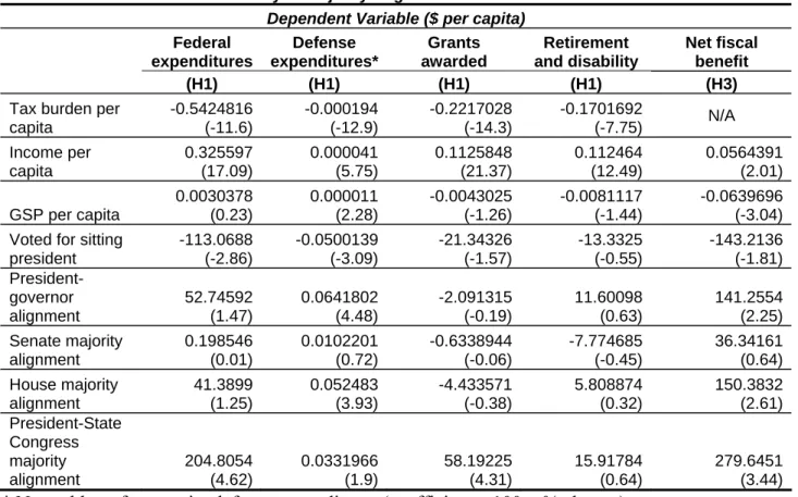
Model 1.1: Total Expenditures (per capita) 46 American States, 1983-2004

Variable Coefficient Standard Error Z P>|z|

Tax burden per capita -0.5424816 4.67E-02 -11.6 0

Income per capita 0.325597 1.91E-02 17.09 0

GSP per capita 0.0030378 1.29E-02 0.23 0.814

Voted for sitting president -113.0688 3.96E+01 -2.86 0.004 President-governor alignment 52.74592 35.7826 1.47 0.14 Senate majority alignment 0.198546 33.29325 0.01 0.995 House majority alignment 41.3899 33.00071 1.25 0.21 President-State Congress majority

alignment 204.8054 44.3402 4.62 0

Population density -3.469659 0.5129692 -6.76 0

2_{The random-effects model (for this model and all subsequent models) was chosen using a Hausman test} for random-effects specification, testing the null hypothesis that the coefficients estimated by the efficient random effects estimator are the same as the ones estimated by the consistent fixed effects estimator. The results were insignificant, with Prob>chi2 greater than .05, and thus justified the use of a random-effects

(23)

Electoral vote per capita 2.60E+08 1.43E+08 1.82 0.068

Senators per capita 2.06E+08 1.76E+08 1.17 0.242

Coastal state 640.3563 168.8857 3.79 0

Constant -514.8069 340.012 -1.51 0.13

Observations = 1012; Groups = 46; Observations per group = 22 R2 (within) = 0.8953 R2 (between) = 0.0049 R2 (overall) = 0.6047 Some important results are summarized below:

- A dollar increase in per capita tax burden decreases the per-capita amount received by the state by 50 cents;

- An increase by a dollar in per capita income increases the per-capita amount received by the state by 32 cents;

- A state that elected the president into office receives less than a state that voted against the sitting president, for any part of a 4-8 year term;

- Alignment variables are not important in the aggregate totals, however, party alignment between the President and the majority party of a State’s Congress yields a $204 per capita increase in total federal expenditures;

- A coastal state receives approximately $640 more per capita than a non-coastal state.

Results for the political variables in the majority alignment model reveals that voting for the sitting President does not have a favorable impact on the state’s total federal

expenditure dollars. Alignment with the house majority is not significant, and would seem to contradict Levitt and Snyder’s (1997) results, as well as their predecessors in the literature. The effect of House majority alignment is perhaps understated in this model. Given that a populous state such as Ohio (17 representatives) or California (53

representatives)3 sends many members, whereas less populous states such as Wyoming have but one representative, the effects of a powerful member of the House are primarily felt within a district, which can be part of a state or the entire state. As the Levitt and Snyder paper indicates, this can be corrected by examining district-by-district

expenditures, using as instrumental variable the out-of-district but in-state total

expenditures received, but a valid data set is only available for 1983-1990. Furthermore, due to decennial reapportionment, it is not possible to conduct district-corrected studies

(24)

for more than ten years. For purposes of this paper, it is difficult to control for the precise geographic impact a member of the house would have on his or her district, as the period studied extends far beyond 1983-1990, the period for which such an instrumental variable method is available. To correct for this, Atlas et al (1995) and Larcinese et al (2005) include the variables senators per capita and electoral vote per capita to correct for the overrepresentation bias. We have included these variables in the regressions. Indeed, this paper is more concerned with global impacts of alignment with the majority or with political party rather than specific determinants for individually powerful members of the federal legislative branch. A previously unstudied variable, party alignment between the President and the controlling party of a state’s congress is significant at the 0% level. Coastal states receive more than non-coastal states; this is primarily due to the larger amounts of spending that are allocated towards coastal defense and are aggregated in the total per-capita expenditure amounts.

Defense Expenditures:

Defense expenditures are computed by totaling the expenditures for all Department of Defense agencies. The following model takes the natural logarithm4 of per-capita defense expenditures as the dependent variable:

Model 2.1: Defense Expenditures (logarithm of per capita amounts) 46 American States, 1983-2004

Tax burden per capita -1.94E-04 0.0000151 -12.9 0

Income per capita 4.03E-05 7.01E-06 5.75 0

GSP per capita 0.0000106 4.67E-06 2.28 0.023

Voted for sitting president -0.0500139 0.0161867 -3.09 0.002 President-governor alignment 0.0641802 0.0143281 4.48 0 Senate majority alignment 0.0102201 0.0141644 0.72 0.471 House majority alignment 0.052483 0.0133454 3.93 0 President-State Congress majority

alignment 0.0331966 0.0174987 1.9 0.058

Electoral vote per capita 154548.8 61569.06 2.51 0.012

Senators per capita -52153.33 87959.37 -0.59 0.553

Coastal state 0.4645287 0.20761 2.24 0.025

Constant 5.823025 0.1578088 36.9 0

4_{Following precedent in Shor (2005), wide disparities amongst states in this spending total can be} smoothed out by taking the natural logarithm. All procurement categories will also be expressed in

(25)

Observations = 1012; Groups = 46; Observations per group = 22 R2 (within) = 0.2481 R2 (between) = 0.0162 R2 (overall) = 0.0311

Some important results are summarized below:

- An increase of $100 in per capita tax burden decreases per-capita defense expenditures by 2%;

- An increase of $1000 in per capita income increases per-capita defense expenditures by 4%;

- An increase of $1000 in GSP per capita increases per-capita defense expenditures by 1%;

- Voting for the sitting president decreases federal defense dollars per capita by 5%; - Party alignment between the president and the governor increases federal defense

spending in the state by 6.4%, while party alignment between the president and the state legislative branch increases defense spending by 3.3%;

- A majority of representatives aligned with the controlling party of the House increases per capita defense spending by 5.2%;

- Less densely populated states receive more than higher-density states; - Coastal states receive 50% more in defense spending than non-coastal states.

Less-wealthy states receive a significantly larger share of the defense spending pie, which could be indicative of the fact that more defense employees also live in those states. Politically, a vote for a sitting president is not significant, while alignment between the governor and the president is very significant. This alignment variable was first studied in the recent Larcinese et al (2006) paper5. Amongst other political variables, alignment with the House majority and President- State congress alignment are significant at the 1% and 5% levels, respectively.

Grants Awarded:

The grants awarded category includes two different types of grants, formula grants and project grants. Formula grants are “allocations of money to States or their subdivisions in accordance with a distribution formula prescribed by law or administrative regulation, for

(26)

activities of a continuing nature not confined to a specific program;”6 while project grants are defined as “the funding, for fixed or known periods, of specific projects or the

delivery of specific services or products without liability for damages for failure to perform. Project grants include fellowships, scholarships, research grants, training grants, traineeships, experimental and demonstration grants, evaluation grants, planning grants, technical assistance grants, survey grants, construction grants, and unsolicited contractual agreements.” This category includes both intergovernmental grants and grants to

individuals.

The regression on grants awarded per capita yields the following model:

Model 3.1: Grants awarded (per capita) 46 American States, 1983-2004

Variable Coefficient Standard Error z P>|z|

Tax burden per capita -0.2217028 0.015477 -14.3 0

Income per capita 1.13E-01 0.0052689 21.37 0

GSP per capita -4.30E-03 0.0034093 -1.26 0.207

Voted for sitting president -21.34326 13.56105 -1.57 0.116 President-governor alignment -2.091315 10.85167 -0.19 0.847 Senate majority alignment -0.6338944 10.42645 -0.06 0.952 House majority alignment -4.433571 11.77089 -0.38 0.706 President-State Congress majority

alignment 58.19225 13.4862 4.31 0

Coastal state 111.4297 40.25515 2.77 0.006

Constant -606.4701 96.26826 -6.3 0

- A state receives 10 cents for every dollar of per capita income; - A state receives 20 cents less per dollar of per capita tax burden;

- The political alignment variable of any significance is the alignment between the president and the state congress, which procures approximately $60 more dollars in grants spending per person;

- Less densely populated states receive more per capita than urbanized states;

(27)

- Coastal states receive $110 more per capita than landlocked states.

The tax burden per capita is negative and significant in both regressions, indicating once again a transfer from the richer-income states to the lower-income states. For every dollar increase in per-capita tax burden, each model predicts a loss to the state of either $3,800 or $3,200, respectively, in federal grants dollars. There is little evidence of a presidential “reward” to the states that placed him in office. The only political variable showing statistical significance is that of President-State Congress party alignment, whereas geographic factors seem to factor heavily into grants spending. A potential explanation could be that components of grants, such as highway spending, are more required in states that cover a wider geographic expanse.

Procurement Spending:

Procurement data, divided into defense procurement and other agency procurement (other procurement) is represented by the value of obligations for contract actions and does not reflect actual government expenditures. Data is coded to the place of performance (state) rather than the location of the primary contractor. Excluded from this category are the amounts for the judicial and legislative branches of government as well as most

intergovernmental transfers of funds. Foreign procurement spending (that is, spending in a foreign country as place of performance) is excluded. Capital expenditures as well as building leases, utilities payment and other services are included. The first model in this category takes the natural logarithm of total procurement per capita as the dependent variable:

Model 4.1: Total procurement (log of per capita amounts) 46 American States, 1983-2004

GSP per capita -5.12E-06 7.00E-06 -0.73 0.464

Voted for sitting president -0.0227638 0.0208042 -1.09 0.274 President-governor alignment 0.0345897 0.0205444 1.68 0.092

Senate majority alignment 0.0059279 0.0192638 0.31 0.758

House majority alignment 0.0602979 0.0175405 3.44 0.001 President-State Congress majority

(28)

Population density -0.0011295 0.0003261 -3.46 0.001 Electoral vote per capita 165869.3 87202.97 1.9 0.057

Senators per capita 28600.22 117926.7 0.24 0.808

Coastal state 0.3865817 0.1829957 2.11 0.035

Constant 5.31957 0.2089126 25.46 0

- An increase in the per capita tax burden of $100 decreases procurement spending by 2%;

- An increase of $1000 in per capita income increases procurement spending by 7.5%;

- Alignment between the president and governor’s political party increases total procurement spending by 3.5%;

- Alignment with the party controlling the House of Representatives increases procurement spending by 6%;

- States with a higher population density receive less, while coastal states receive more.

The total procurement spending category exhibits the same relationship with income per capita and tax burden per capita as has many other spending categories. In model 4.1, the variables of importance are alignment variables – between the President and a state’s governor, and alignment with the House majority. The literature shows an extensive focus on the role of the House of Representatives in discretionary spending, yet the results here indicate that these other studies may “have failed to incorporate data from other sources of influence at different levels of analysis…” and that “…predictors at different levels of analysis affect our conclusions regarding partisan effects on distributive politics.” (Shor 2005)

Defense Procurement:

Disaggregating total procurement spending into two subgroups, we first examine federal defense procurement expenditures. This model takes the natural logarithm of defense procurement per capita as dependent variable.

(29)

Model 5.1: Defense procurement (log of per capita amounts) 46 American States, 1983-2004

Income per capita 0.0000734 0.0000128 5.75 0

GSP per capita -5.63E-06 8.73E-06 -0.65 0.519

Voted for sitting president -0.0534968 0.0250464 -2.14 0.033 President-governor alignment 0.0869665 0.0246185 3.53 0 Senate majority alignment 0.0485212 0.0230064 2.11 0.035 House majority alignment 0.0949392 0.0219298 4.33 0 President-State Congress majority

alignment 0.0404447 0.0298959 1.35 0.176

Population density -0.0004652 0.0004073 -1.14 0.253 Electoral vote per capita 244266.3 107884.9 2.26 0.024

Senators per capita -219754.4 145129.4 -1.51 0.13

Coastal state 0.4705112 0.2383926 1.97 0.048

Constant 4.885822 0.2521169 19.38 0

Observations = 1012; Groups = 46; Observations per group = 22 R2 (within) = 0.1766 R2 (between) = 0.0141 R2 (overall) = 0.0371 Results include:

- An increase in tax burden per capita of $100 would decrease defense procurement spending by 2.7%;

- An increase in income per capita of $1000 would increase defense procurement by 7.3%;

- A vote for the sitting president decreases the amount received by 5.3%; - Alignment between the president and a state’s governor increases the amount

received by a state by 8.7%;

- Alignment with the Senate majority and the House majority shows an increase in federal defense procurement spending of 4.9% and 9.5%, respectively;

- A coastal state receives 47% more defense procurement dollars than a non-coastal state.

The same effects shown in the total procurement spending model hold in this model, with political alignment and the impact of the president showing statistical significance all at the 5% level or 1% level.

(30)

Other Procurement:

Differencing the defense procurement from total procurement yields the category of other procurement spending. The first model uses the natural logarithm of other procurement spending per capita as the dependent variable, producing the following results:

Model 6.1: Other procurement (log of per capita amounts) 46 American States, 1983-2004

GSP per capita 9.36E-06 9.18E-06 1.02 0.308

Voted for sitting president 0.0187768 0.0237915 0.79 0.43 President-governor alignment -0.0218048 0.0246648 -0.88 0.377 Senate majority alignment -0.0203954 0.0207546 -0.98 0.326 House majority alignment -0.0365785 0.0196383 -1.86 0.063 President-State Congress majority

alignment -0.0085568 0.0258438 -0.33 0.741

Electoral vote per capita -18301.22 72473.49 -0.25 0.801

Senators per capita 422485.2 137989.9 3.06 0.002

Coastal state 0.4286302 0.1600995 2.68 0.007

Constant 3.831463 0.2226073 17.21 0

- An increase of $100 in the tax burden per capita yields a 1% decrease in other procurement spending per capita;

- An increase of $1000 in the income per capita yields a 6% increase in other procurement spending;

- Political alignment variables are not at all significant, other than alignment with the House of Representatives majority, which shows a 3% decrease in other procurement spending per capita;

- The variable Senators per capita, which shows the effect by “overrepresented” states, indicates that they are favored in other procurement spending.

Once again, the same tendencies hold for the income per capita and the tax burden per capita. The majority alignment model yields but one statistically significant and negative impact on the non-defense procurement dollars received, which is alignment with the

(31)

Retirement and Disability Payments:

Retirement and disability data includes federal employee retirement and disability benefits (including military and diplomatic personnel) and all Social Security payments. The first model takes per capita retirement and disability payments as dependent variable; the regression reveals the following information:

Model 7.1: Retirement and Disability (per capita) 46 American States, 1983-2004

GSP per capita -8.11E-03 0.0056385 -1.44 0.15

Voted for sitting president -13.3325 24.31769 -0.55 0.584 President-governor alignment 11.60098 18.4597 0.63 0.53 Senate majority alignment -7.774685 17.20426 -0.45 0.651 House majority alignment 5.808874 18.05438 0.32 0.748 President-State Congress majority

alignment 15.91784 24.85702 0.64 0.522

Senators per capita -6.62E+07 5.09E+07 -1.3 0.193

Coastal state 83.37106 53.51849 1.56 0.119

Constant 14.66442 117.6832 0.12 0.901

- A dollar increase in the tax burden per capita yields a decrease of 17 cents per capita in retirement and disability spending, while a dollar increase in income per capita increases the amount received by 11 cents;

- There is no significant political effect observed on the allocation of retirement and disability spending to the states;

- States with a higher population density receive less than states with a lower population density.

It is logical that retirement and disability payments to the states do not seem to be politically influenced, as both these payments are largely formula based. A state with a greater population density could conceivably provide the same level of service in a state

(32)

with lower population density by taking advantage of the economies of scale offered by a more urbanized population.

Other Payments:

The spending category “Other Payments” includes other direct payments to individuals other than retirement and disability and direct payments that are not for individuals. The former category includes excess earned income tax credit payments, payments to state unemployment trust funds, and interest subsidies for family education loans. The latter category includes the administration costs of the federal family education loan program, crop insurance indemnity payments and crop subsidies, all procurement and non-salary postal service expenditures, federal contributions to employee life and health insurance programs, along with other smaller programs of a similar nature. The first model uses other payments in per-capita terms as dependent variable:

Model 8.1: Other Payments 46 American States, 1983-2004

GSP per capita -9.31E-03 0.0044321 -2.1 0.036

Voted for sitting president -44.17144 17.78916 -2.48 0.013 President-governor alignment 11.0443 16.9816 0.65 0.515 Senate majority alignment -9.73557 17.85796 -0.55 0.586 House majority alignment -11.67391 15.92125 -0.73 0.463 President-State Congress majority

alignment 80.61363 20.56637 3.92 0

Population density -0.4287709 0.1244383 -3.45 0.001 Electoral vote per capita -2.45E+07 4.69E+07 -0.52 0.602

Coastal state 37.5652 38.30657 0.98 0.327

Constant -448.9418 122.6501 -3.66 0

- A dollar increase in income per capita increases other payments by 10 cents, while a dollar increase in per capita tax burden decreases other payments by 12 cents;

(33)

- Alignment between the sitting president and the controlling party of the state’s Congress increases other payments to the state by $81 dollars per capita; - More densely populated states receive less than sparsely populated states.

Although other payments to states can include more pork-barrel type spending items, a look at the majority alignment model shows the determinants to be largely geographic and economic. The variable showing party alignment between the controlling party of a state’s Congress and the president, which is new to the literature, is significant at the 1% level.

Hypothesis 2: Pure party affiliation on federal and state levels is an important determinant for certain federal spending categories

In this section, we will model the dependent variables in total dollar terms. The choice is rather arbitrary, as the literature shows transfers in a partisan model modeled as

percentage of total budget (Budge and Hofferbert, 1990) or in total dollar terms (Levitt and Snyder, 1995). We have chosen the latter method, with a logarithmic transformation in procurement and defense-related categories.

Total expenditures:

This is the aggregate of all government spending and obligations. We again use a random-effects7 GLS model with robust standard errors, taking total expenditures in dollar amounts as dependent variable.

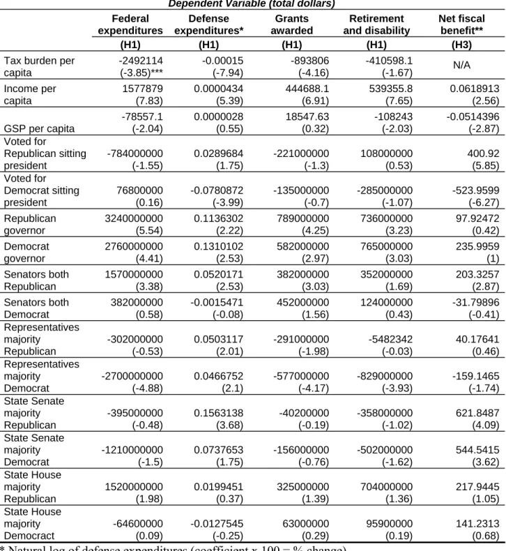
Model 1.2: Total expenditures (total dollars) 46 American States, 1983-2004

Population 2990.007 490.2887 6.1 0

Population2 0.0000811 0.0000157 5.16 0

Tax burden per capita -2492114 647042.1 -3.85 0

Income per capita 1577879 201559.4 7.83 0

7_{The random-effects model (for this model and all subsequent models) was chosen using a Hausman test} for random-effects specification, as we did for the previous subsection.

(34)

Senators per capita -3.10E+15 1.52E+15 -2.04 0.041

GSP per capita -78557.1 160120.7 -0.49 0.624

Population density -1393213 2740475 -0.51 0.611

Voted for Republican sitting president -7.84E+08 5.05E+08 -1.55 0.121 Voted for Democrat sitting president 7.68E+07 4.91E+08 0.16 0.876

Republican governor 3.24E+09 5.86E+08 5.54 0

Democrat governor 2.76E+09 6.26E+08 4.41 0

Senators both Republican 1.57E+09 4.66E+08 3.38 0.001

Senators both Democrat 3.82E+08 6.64E+08 0.58 0.565

Representatives majority Republican -3.02E+08 5.69E+08 -0.53 0.595 Representatives majority Democrat -2.70E+09 5.52E+08 -4.88 0 State Senate majority Republican -3.95E+08 8.21E+08 -0.48 0.631 State Senate majority Democrat -1.21E+09 8.06E+08 -1.5 0.135 State House majority Republican 1.52E+09 7.71E+08 1.98 0.048 State House majority Democrat -6.46E+07 7.51E+08 -0.09 0.931

Swing State 2667540 5.75E+08 0 0.996

Coastal 9.75E+08 1.12E+09 0.87 0.383

Constant -2.43E+10 3.56E+09 -6.83 0

- A dollar increase in per capita tax burden decreases a state’s total federal expenditures by $2.4 million;

- An dollar increase in per capita income increases the amount received by the state by $1.5 million;

- A Republican governor receives $480 million more than a Democrat counterpart; - Representatives that are in majority Democrat bring $2.7 billion less than a split

or majority Republican House delegation;

- A State House of Representatives that is majority Republican indicates $1.52 billion more in total federal expenditures.

Results concerning the allocation of total spending determined by pure party alignment model are not particularly noteworthy, beyond the economic, population and geographic effects similarly captured in the majority alignment model. Notably, having a State’s two members of the Senate aligned with the Republican Party has a significant positive impact on the total funds received by the State. A majority of Democrat Representatives yield a significant negative impact on the total federal funds received by the state. In the

(35)

aggregate of federal expenditures, it is the federal legislative branch that seems to have the most impact.

Defense Expenditures:

Defense expenditures are computed by totaling the expenditures for all Department of Defense agencies. The following model takes the natural logarithm8 of total defense expenditures as the dependent variable:

Model 2.2: Defense Expenditures (logarithm of total dollars) 46 American States, 1983-2004

Population 1.29E-07 1.58E-08 8.19 0

Population2 -2.51E-15 3.33E-16 -7.54 0

Income per capita 0.0000434 8.06E-06 5.39 0

Electoral vote per capita 165038.9 65697.8 2.51 0.012

Senators per capita -660543.2 99880.54 -6.61 0

GSP per capita 2.80E-06 5.12E-06 0.55 0.584

Voted for Republican sitting

president 0.0289684 0.0165605 1.75 0.08

Voted for Democrat sitting president -0.0780872 0.0195658 -3.99 0

Republican governor 0.1136302 0.0510719 2.22 0.026

Senators both Republican 0.1310102 0.0517908 2.53 0.011

Democrat governor 0.0520171 0.0205373 2.53 0.011

Senators both Democrat -0.0015471 0.0198169 -0.08 0.938 Representatives majority

Republican 0.0503117 0.0250774 2.01 0.045

Representatives majority Democrat 0.0466752 0.0222688 2.1 0.036 State Senate majority Republican 0.1563138 0.0424886 3.68 0 State Senate majority Democrat 0.0737653 0.0421392 1.75 0.08 State House majority Republican 0.0199451 0.0539783 0.37 0.712 State House majority Democrat -0.0127545 0.0512448 -0.25 0.803

Swing State -0.033701 0.017217 -1.96 0.05

Coastal 0.5044113 0.2350721 2.15 0.032

Constant 20.52511 0.1935294 106 0

- An increase of $100 in per capita tax burden decreases total defense expenditures by 1.5%;

- An increase of $1000 in per capita income increases defense expenditures by 4%;

(36)

- An increase of $1000 in GSP per capita increases defense expenditures by 2.8%; - Voting for the sitting Republican president decreases expenditures by 3%; - Voting for the sitting Democrat president decreases expenditures by 7.8%; - Party alignment between the president and the governor increases federal defense

spending in the state by 6.4%, while party alignment between the president and the state legislative branch increases defense spending by 3.3%;

- Delegates to the House of Representatives aligned with the Republicans receive 0.5% more than representatives aligned with the Democrats;

- Less densely populated states receive more than higher-density states; - Coastal states receive 50% more in defense spending than non-coastal states.

Similar results were obtained in this model (compared to the majority alignment model 2.1) with the results for the effects of common explanatory variables. This model, a party alignment model of defense expenditures, reveals that a vote for a Republican president has a very significant impact on defense-allocated expenditures to a state whereas a state that voted for a Democratic president would see a statistically significant drop. A very similar effect is observed with the party alignment of a state’s two senators, with a positive impact for Republican alignment compared with senators split between the two parties or two Democratic senators. This result could reflect the spending priorities of the parties during this time period encompassing the end of the Cold War and the beginning of early 21st_{century neoconservative military interventions and an increase in security}

related spending. This will be discussed in greater depth in the following section.

Grants Awarded:

The regression on total dollars of grants awarded yields the following model:

Model 3.2: Grants awarded (total dollars) 46 American States, 1983-2004

Population 63.08007 203.9006 0.31 0.757

Population2 0.0000399 5.96E-06 6.69 0

Tax burden per capita -893806 214832.3 -4.16 0

(37)

Population density 1839943 1051242 1.75 0.08 Voted for Republican sitting

president -2.21E+08 1.70E+08 -1.3 0.195

Voted for Democrat sitting president -1.35E+08 1.94E+08 -0.7 0.486

Republican governor 7.89E+08 1.86E+08 4.25 0

Democrat governor 5.82E+08 1.96E+08 2.97 0.003

Senators both Republican 3.82E+08 1.26E+08 3.03 0.002

Senators both Democrat 4.52E+08 2.90E+08 1.56 0.118

Representatives majority

Republican -2.91E+08 1.47E+08 -1.98 0.048

Representatives majority Democrat -5.77E+08 1.38E+08 -4.17 0 State Senate majority Republican -4.02E+07 2.08E+08 -0.19 0.847 State Senate majority Democrat -1.56E+08 2.04E+08 -0.76 0.445 State House majority Republican 3.25E+08 2.34E+08 1.39 0.164 State House majority Democrat 6.30E+07 2.20E+08 0.29 0.774

Swing State -1.34E+08 1.78E+08 -0.75 0.452

Coastal -6.56E+08 3.98E+08 -1.65 0.099

Constant -6.03E+09 1.29E+09 -4.66 0

- A state receives $440,000 more in grants with a dollar increase in per-capita income;

- A state collects $890,000 less in grants per dollar of per capita tax burden; - A Republican governor brings $207 million more than a Democrat governor; - Two Democrat senators bring $70 million more than two Republican senators,

and $452 million more than a split senate delegation;

- More densely populated states receive more in total dollars than states with a lower population density;

- Coastal states receive $656 million less in total dollars than landlocked states.

Population is not a significant variable in this category of spending. Although many grants are formula based, project-based block grants are also included in this category, which are largely determined by the infrastructure needs of a state, an to a certain extent, by pork barrel politics,9 and could thus mitigate the effects of a state’s population. The tax burden per capita is significant, indicating once again a transfer from the richer-income states to the lower-richer-income states, although the increase in richer-income would mitigate

(38)

the effect of the increased taxes10. This party alignment model shows that Senators

aligned with either party have a positive impact on the grants awarded to their home state. On the other side of Capitol Hill, in the House of Representatives, the party alignment variables show a negative impact in grants allocated, indicating that a split delegation would receive more in grants allocated to the state11.

Procurement Spending:

Procurement data is divided into defense procurement and other agency procurement. We will first examine this category in its aggregate. Model 4.2 takes the natural logarithm of total procurement dollars to a state as the dependent variable:

Model 4.2: Total procurement (log of total dollars) 46 American States, 1983-2004

Population 1.52E-07 1.99E-08 7.61 0

Population2 -3.01E-15 4.35E-16 -6.92 0

Electoral vote per capita 148930.4 89947 1.66 0.098

Senators per capita -479749.9 135018.1 -3.55 0

GSP per capita -0.0000132 7.16E-06 -1.84 0.066

Voted for Republican sitting president 0.0448229 0.0204751 2.19 0.029 Voted for Democrat sitting president -0.0688157 0.0253746 -2.71 0.007 Republican governor 0.1786423 0.0561854 3.18 0.001

Democrat governor 0.199523 0.0573112 3.48 0

Senators both Republican 0.0501997 0.0275168 1.82 0.068

Senators both Democrat 0.0162227 0.028652 0.57 0.571 Representatives majority Republican 0.0670286 0.031615 2.12 0.034 Representatives majority Democrat 0.0195326 0.0302592 0.65 0.519 State Senate majority Republican 0.1352461 0.0587794 2.3 0.021 State Senate majority Democrat 0.0597323 0.0577964 1.03 0.301 State House majority Republican 0.0587379 0.0623499 0.94 0.346 State House majority Democrat 0.0095875 0.0592178 0.16 0.871

Swing State -0.0396704 0.0238295 -1.66 0.096

Coastal 0.4256061 0.2508402 1.7 0.09

Constant 19.91405 0.2596142 76.71 0

10_{Assume that a $100 increase in per capita income increases the per capita tax burden by $30. All other} things equal, the net increase in total grants received would be (100*440,000)-(30*890,000)= $18.3 million