Weakening of Jupiter’s main auroral emission
during January 2014
S. V. Badman1, B. Bonfond2, M. Fujimoto3, R. L. Gray1, Y. Kasaba4, S. Kasahara3, T. Kimura5, H. Melin6, J. D. Nichols6, A. J. Steffl7, C. Tao8, F. Tsuchiya4, A. Yamazaki3, M. Yoneda4,9, I. Yoshikawa10, and K. Yoshioka11
1Physics Department, Lancaster University, Lancaster, UK,2Laboratoire de Physique Atmosphérique et Planétaire, Département AGO, Université de Liège, Liège, Belgium,3Institute of Space and Astronautical Science, Sagamihara, Japan, 4Department of Geophysics, Graduate School of Science, Tohoku University, Sendai, Japan,5RIKEN, Wako, Japan, 6Department of Physics, University of Leicester, Leicester, UK,7Department of Space Studies, Southwest Research Institute, Boulder, Colorado, USA,8NICT, Tokyo, Japan,9Kiepenheuer Institute for Solar Physics, Freiburg im Breisgau, Germany, 10Department of Complexity Science and Engineering, University of Tokyo, Tokyo, Japan,11Graduate School of Science, University of Tokyo, Tokyo, Japan
Abstract
In January 2014 Jupiter’s FUV main auroral oval decreased its emitted power by 70% and shifted equatorward by ∼1∘. Intense, low-latitude features were also detected. The decrease in emitted power is attributed to a decrease in auroral current density rather than electron energy. This could be caused by a decrease in the source electron density, an order of magnitude increase in the source electron thermal energy, or a combination of these. Both can be explained either by expansion of the magnetosphere or by an increase in the inward transport of hot plasma through the middle magnetosphere and its interchange with cold flux tubes moving outward. In the latter case the hot plasma could have increased the electron temperature in the source region and produced the intense, low-latitude features, while the increased cold plasma transport rate produced the shift of the main oval.1. Introduction
Auroral images provide a valuable way to remotely observe magnetospheric dynamics. At the gas giant Jupiter there are distinct regions of auroral emissions corresponding to different regions of the magneto-sphere. At the lowest latitudes are the auroral footprint spots of the moons Io, Europa, and Ganymede, which are caused by the perturbation of the planet’s magnetic field as it rotates past these conducting bodies [Connerney et al., 1993; Clarke et al., 2002; Bonfond, 2012]. The main emission encircling the magnetic poles is associated with magnetosphere-ionosphere coupling currents acting to transfer angular momentum from the planet to the subcorotating iogenic plasma in the middle magnetosphere at ∼20–30 RJ[Cowley and Bunce, 2001; Hill, 2001; Grodent et al., 2003a]. The dynamic, patchy “polar” region inside the main emission may partly map to field lines in the outer magnetosphere or connect to the interplanetary magnetic field in the solar wind [Pallier and Prangé, 2001; Gladstone et al., 2002; Grodent et al., 2003b; Vogt et al., 2011]. A diffuse equa-torward arc is sometimes apparent and corresponds to a transition at 10–17 RJin the magnetosphere from field-perpendicular (smaller radial distances) to field-aligned (larger radial distances) electron distributions, where the radial distance of the transition varies from orbit to orbit. At radial distances outside the transition, electrons are thought to be scattered to the field-aligned distribution (and thus into the loss cone) by whistler waves [Tomás et al., 2004; Radioti et al., 2009]. Longitudinally confined, diffuse “low-latitude” emissions are often observed in a similar region between the main emission and the Io footprint and are possibly associ-ated with injections of energetic electrons detected by Galileo at radial distances of 9–27 RJ[Mauk et al., 1999, 2002; Bonfond et al., 2012; Dumont et al., 2014].
The components of the aurora display variability on timescales of seconds to weeks, which can be inter-preted as a response to solar wind influence superposed on internal magnetospheric dynamics [e.g., Nichols et al., 2009]. A compression of the magnetosphere by the solar wind is expected to cause the main emis-sion to dim as the mass-loaded field lines conserve angular momentum as they are displaced radially inward [Southwood and Kivelson, 2001; Cowley et al., 2007]. However, the timescales on which the compression prop-agates through the magnetosphere and the neutral atmosphere responds are not well constrained so that
RESEARCH LETTER
10.1002/2015GL067366
Key Points:
• Jupiter’s auroral power decreased by 70% over 2 weeks of observations by the Hubble Space Telescope • Could be caused by expansion of the
magnetosphere or increase in hot plasma transport
• Aurora is variable without enhanced Io volcanism or solar wind pressure implications for Juno
Correspondence to:
S. V. Badman,
s.badman@lancaster.ac.uk
Citation:
Badman, S. V., et al. (2016), Weak-ening of Jupiter’s main auroral emission during January 2014,
Geophys. Res. Lett., 43, 988–997,
doi:10.1002/2015GL067366.
Received 9 DEC 2015 Accepted 22 JAN 2016
Accepted article online 28 JAN 2016 Published online 10 FEB 2016
©2016. The Authors.
This is an open access article under the terms of the Creative Commons Attribution License, which permits use, distribution and reproduction in any medium, provided the original work is properly cited.
brief increases in the main oval field-aligned currents may also occur [Cowley et al., 2007; Yates et al., 2014]. Cassini observations demonstrated auroral brightenings related to solar wind compressions at Jupiter, but the auroral observations did not have sufficient spatial resolution to identify which auroral region(s) became brighter [Gurnett et al., 2002; Pryor et al., 2005]. Overall, ambiguity in the timing of solar wind conditions arriving at Jupiter and the limited cadence of auroral imaging have not yet allowed the full auroral response to solar wind compressions or rarefactions to be conclusively identified [Nichols et al., 2007, 2009; Clarke et al., 2009].
The auroral emissions also demonstrate a response to changes in the inner magnetosphere related to the mass loading and field stretching. Grodent et al. [2008] and Bonfond et al. [2012] suggested that movement of the main oval to lower latitudes, observed in images separated by months or years, could be caused by a change in the magnetic field stretching or an inward shift in the corotation breakdown boundary. These effects were related to an increase in mass loading from Io [e.g., Yoneda et al., 2010]. An increase in the outflow rate of iogenic plasma is expected to affect the intensity of the main aurora, but whether it increases or decreases depends on the model employed [Nichols and Cowley, 2003; Nichols, 2011; Ray et al., 2012].
In this study a 2 week sequence of auroral observations is used to investigate the variation in both the intensity and location of Jupiter’s aurora in relation to magnetospheric conditions.
2. Auroral Observations
2.1. Data
Jupiter’s northern aurora was observed using the Hubble Space Telescope (HST) Space Telescope Imaging Spectrograph (STIS) during 14 “visits” (i.e., observation sequences) over 16 days in January 2014. Images were acquired using the SrF2 longpass filter, which excludes hydrogen Lyman alpha emission at 121.6 nm but covers the H2Lyman and Werner bands in the range 125–190 nm. The data were processed using a pipeline
developed at Boston University, including dark count subtraction, flat-fielding, geometric distortion correc-tion, scaling to a standard opposition distance between HST and Jupiter of 4.2 AU, and subtraction of an empirical disk background [Clarke et al., 2009; Nichols et al., 2009]. The images were projected onto a plane-tocentric latitude and System III longitude grid at an emission altitude of 240 km above the 1 bar pressure level [Vasavada et al., 1999]. The spatial uncertainties in the projected images come mainly from determining the center of the planet and the “stretching” of pixels close to the planet’s limb; these uncertainties are fully described by Grodent et al. [2003a], who show that the inaccuracies are typically ∼1∘ for the main auroral oval observation geometry.
Observations were made in two sets of duration ∼ 700 s on each HST visit. For images shown in this study the photon counts were integrated over intervals of 100 s to achieve both good temporal resolution and signal-to-noise ratio. The counts were converted to a brightness in kiloRayleigh using the conversion factor given by Gustin et al. [2012] of 1kR = 2.211 × 10⁻⁴counts. This assumes a color ratio of 2.5 across the auroral
region, as inferred from STIS spectral observations made during the same campaign (C. Tao et al., Variation of Jupiter’s aurora observed by Hisaki/EXCEED: 1. Observed characteristics of auroral electron energies com-pared with HST/STIS observations, submitted manuscript Journal of Geophysical Research: Space Physics, 2016), where the color ratio is the ratio of intensity in a UV wavelength band unabsorbed by atmospheric hydrocar-bons (155–162 nm) to the intensity in an absorbed band (123–130 nm), i.e., a measure of auroral electron penetration depth and hence electron energy. The auroral powers quoted below correspond to the auroral H2emission across a wavelength range of 70–180 nm [Gustin et al., 2012].
2.2. Auroral Morphology
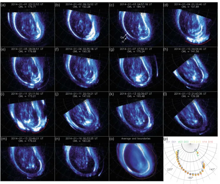
One image from each of the 14 HST visits is shown in Figure 1. At the start of the campaign, on days 1–3, the main oval was bright and composed of narrow arcs at most longitudes (Figures 1a–1c).
On day 4 (Figure 1d) the auroral morphology was noticeably different: the main oval was dimmer at all longitudes than in the previous images, and the brightest emission came from an extended region of diffuse emission at longitudes 140–190∘. This region is highlighted by the red line on the image.
The diffuse emission was fixed in System III longitude, i.e., was corotating with the planet, and the Ganymede footprint could be observed moving out of this western edge of the diffuse structure over the sequence, although it is not distinct in the snapshot shown. The diffuse emission extended across ∼3–4∘ latitude, from
Figure 1. Gallery of selected images of Jupiter’s northern UV aurora imaged by HST/STIS in January 2014. (a–n) The time and CML for each image are labeled. The
images have been projected onto a polar grid at an altitude of 240 km above the 1 bar pressure level and are viewed from above the north pole with System III longitude 180∘at the bottom of each panel. A latitude-longitude grid with spacing of 10∘is superposed. The images are plotted using a log color scale saturated at 500 kR. Red lines on Figures 1d and 1i mark features described in the text, while the arrowed labels in Figure 1c indicate the Io and Ganymede footprints. (o) The average intensity derived from all images. The red contours show the boundaries of the three auroral regions: polar, main oval, and low latitude, as described in the text. (p) The location of the peak brightness at selected longitudes, tracing out the main oval, for visits 1, 3, 13, and 14 on days 1, 3, 13, and 16, as labeled.
the main oval to ∼1∘ poleward of the Io footprint contour (the Io footprint itself was not captured in these images).
Approximately 25 h later, on day 5, the diffuse equatorward feature had disappeared and the main oval was of slightly higher intensity again (Figure 1e). Similar morphologies were observed in the subsequent images taken on days 6, 7, and 10, shown in Figures 1f–1h.
The first of two sets of images on day 11 (Figure 1g) shows another very different auroral morphology. The main oval region was formed of bright patches. Large regions of equatorward emission were observed, extending from one of the main oval patches at longitudes 185–190∘ and as a distinct equatorward feature at longitudes 135–170∘ (highlighted by red lines). The Ganymede footprint was observed to move between these two structures over the interval but again is not visible in the snapshot shown. Some bright polar fea-tures were observed. The second set of images on day 11 began ∼18 h later and reveal that all regions of the aurora had become fainter over this interval.
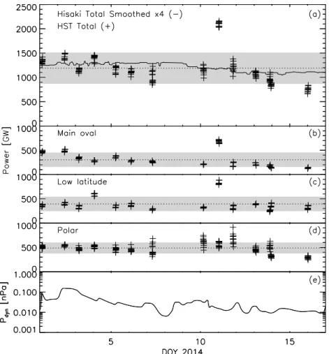
Figure 2. Auroral power and solar wind dynamic pressure during 1–16 January 2014. (a) Total emitted FUV auroral
power observed by HST/STIS (crosses), their mean (dotted line), and standard deviation about the mean (shading). The solid line shows the total EUV auroral power observed by Hisaki/EXCEED, smoothed by a running median with a window of 39.7 h (four Jovian rotations), and scaled by a factor of 4. (b–d) Emitted power from the main oval, low-latitude, and polar regions, as defined in the text. (e) Solar wind dynamic pressure at Jupiter propagated using a 1-D MHD model.
The main oval remained relatively dim and accompanied by the faint secondary arc for the rest of the obser-vations on days 13 and 16. The brightest arcs along the main oval were in the longitude sector 100–160∘. Some equatorward patches were also observed (e.g., early on day 13), but they were not as large or bright as those observed on days 4 and 11.
It is clear from the images and above discussion that many intriguing features were observed in different regions of the aurora, representing different magnetospheric dynamics, over the duration of the campaign in January 2014. In the subsequent sections we focus on one aspect of the auroral variability: the power emitted from different regions as a function of time.
2.3. Auroral Power
To quantify the variability of the auroral power, the auroral region was subdivided into different latitudinal regions, corresponding to different source regions in the magnetosphere, following Nichols et al. [2009]. The main oval region was defined as a strip 2∘ wide in latitude, centered on the average main oval determined from all images. The polar region was defined as the region poleward of this, and the low-latitude region was the region equatorward of the main oval region, up to a contour 1.5∘ poleward of the Io footprint contour defined by Bonfond et al. [2009]. The average emission intensity over the campaign is shown in Figure 1o with these boundaries overlaid.
The fraction of Jupiter’s auroral region visible to HST varies as the planet rotates because of the offset of the magnetic axis from the spin axis. This variability needs to be accounted for so that powers from different images can be compared. To achieve this, the observed powers were scaled by a function representing the
observable fraction of the auroral region for all central meridian longitudes (CMLs), following the method described by Nichols et al. [2009]. This assumes that the auroral emission is roughly homogenous over each region. The corrected powers are shown as a function of time in Figure 2. Figures 2b–2d present the power emitted in the main oval, low-latitude, and polar regions, respectively. The dotted lines show the mean value across the observations, and the grey shading indicates the standard deviation from this value. The variation of the total power summed over these regions is shown by the crosses in Figure 2a for each 100 s integration. The black dotted line and grey shading in Figure 2a represent the mean total power and the standard deviation of the values over the campaign.
The power emitted from the main oval declined gradually over the campaign, with the exception of visit 9 on day 11, during which a localized bright patch extended across the main oval latitudes (see Figure 1i). This feature was the brightest of the campaign and affected the power in both the main oval and low-latitude regions. The average main oval emitted power on days 1–2 was ∼480 GW, decreasing to ∼170 GW on days 13–16.
The polar region also emitted low powers at the end of day 13 and on day 16; however, a general decrease in the polar power over the whole campaign is not apparent. The overall standard deviation of the polar emitted power was lower than that of the main oval power, but individual days show much greater variation, i.e., days 7–13. This indicates that the intensity of the polar region is highly variable on minute timescales.
The low-latitude region showed little variation in emitted power over the campaign (average 395 GW) with the exception of two large increases on days 4 and 11. The total power also shows a net decrease in emitted power over the campaign, in line with the reduced contribution from the main oval. It falls from an average power of 1380 GW on days 1 and 2 to an average of 900 GW on days 13 and 16.
The decrease in the total auroral power captured by the HST observations was also detected by the Hisaki Extreme Ultraviolet Spectroscope for Exospheric Dynamics (EXCEED) mission [Yoshikawa et al., 2014; Yamazaki et al., 2014], which monitored Jupiter’s EUV auroral emission quasi-continuously during December 2013 to March 2014 [Kimura et al., 2015]. The total EUV auroral power over 90–148 nm detected by Hisaki is repre-sented in Figure 2a by the solid line, where the values have been averaged using a running median with window 39.7 h, i.e., four jovian rotations, to remove the quasi-sinusoidal variation imposed by the planetary rotation, and scaled by a factor of 4 for ease of viewing on this scale. (Full details of the Hisaki auroral power estimation are given by Kimura et al. [2015].) The smoothed EUV power decreased from ∼320 GW on days 1–2 to ∼270 GW on days 13–16. A decrease in auroral power over these timescales was previously identified from International Ultraviolet Explorer observations [Prangé et al., 2001], which also lacked spatial resolution. The HST observations provide spatially resolved images from which we can determine that the overall decrease in power over this 2 week interval was mainly driven by a decrease in the emission from the main oval.
2.4. Auroral Location
Figure 1p shows the location of the peak brightness at certain longitudes, tracing out the main oval, for selected HST visits at the start (1 and 3 January) and end (13 and 16 January) of the interval. The position of the peak brightness had shifted slightly equatorward, by an average of 1∘, at the end of the campaign compared to at the start. For comparison, the latitude of the main oval can vary over a full visit (2 × 700 s) by 0–0.5∘ on average, while the maximum displacement along a given line of longitude across all visits is 2.5∘ (excluding regions where the main oval could not be precisely located because of, e.g., proximity to the edge of the field of view or where the auroral oval was particularly faint or diffuse). We take the 1∘ shift between days 1 and 16 as representative of the long-term equatorward shift while acknowledging that this neglects variability on shorter timescales. The magnitude of the observed shift is comparable to the expansion of the main oval previously identified over longer intervals [Grodent et al., 2008; Bonfond et al., 2012]. Although the magnitude of the shift is comparable to the spatial uncertainties described above, the fact that it represents a long-term trend rather than random fluctuations leads us to consider this shift as real.
3. Causes of Auroral Variability
A decrease in the main oval intensity would be caused by a reduction in auroral electron energy flux deposited in the upper atmosphere. This is related to the magnitude of the field-aligned current linking the ionosphere and the corotation breakdown region in the equatorial magnetosphere. A decrease in the mass loading of the field lines or a reduction in their radial stretching could result in a lower auroral field-aligned current
[e.g., Nichols, 2011]. One possible cause for a reduction in the radial stretch of the magnetic field lines is a global compression of the magnetosphere by the arrival of a high-pressure solar wind region. The solar wind conditions at Jupiter can be estimated using a 1-D MHD code [Tao et al., 2005] to propagate the solar wind measured near Earth out to 5 AU. The uncertainty in the arrival times is less than ±24 h at this time because of the small (<25∘) Earth-Sun-Jupiter angle. The propagated dynamic pressure is presented in Figure 2e and shows that the HST auroral observations took place during an interval of decreasing solar wind pressure and radial velocity. This would result in an expansion of the magnetosphere and, assuming conservation of angular momentum, associated increase in the auroral currents [Cowley et al., 2007; Yates et al., 2014], opposite to what is inferred from the auroral observations. We therefore examine other possible causes of a decrease in field-aligned current and auroral electron energy flux.
Using Hisaki/EXCEED spectra, Tao et al. [2015, also submitted manuscript, 2016] showed that the mean energy of the electrons precipitating into the main oval remained roughly constant over this campaign. This implies that the observed decrease in precipitating energy flux is associated with a decrease in electron number flux (equivalent to the current density) rather than electron energy. The variation in magnetospheric param-eters which could cause the observed decrease in the auroral current density can be examined using the Knight [1973] relation. The maximum upward current density that can be carried by magnetospheric electrons without field-aligned acceleration is
j||0= eN ( W th 2𝜋me )1∕2 , (1)
where e and meare the charge and mass of the electron and N and Wthare the number density and thermal
energy of the source electron population in the magnetosphere. This relation assumes a full downgoing loss cone and empty upgoing loss cone. The field-aligned energy flux of these electrons precipitating into the ionosphere is Ef 0= 2NWth ( W th 2𝜋me )1∕2 . (2)
The current density can be enhanced by a field-aligned potential drop to produce the current required in the middle magnetosphere coupling system. Using the linear approximation to the Knight relation, the enhanced current density just above the ionosphere, j||, results in an increased field-aligned energy flux of the precipitating electrons given by Lundin and Sandahl [1978]:
Ef= Ef 0 2 [(j || j||0 )2 + 1 ] . (3)
The energy flux can be estimated from the observed brightness of the main oval, using the relation that 1 mW m−2incident energy flux produces 10 kR of auroral intensity [Gustin et al., 2012, and references therein].
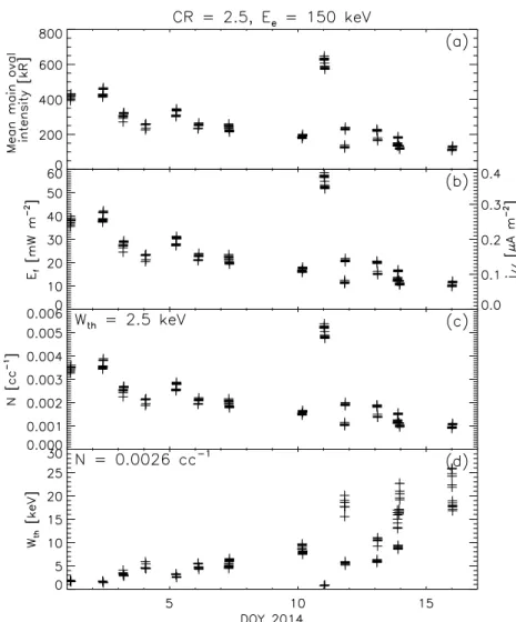
The mean intensity in the main oval region and the derived electron energy flux are shown as a time series in Figures 3a and 3b. The right-hand axis of Figure 3b indicates the corresponding current density j||, determined by assuming that the energy flux is deposited by electrons with mean energy< W > = 150 keV as indicated by spectral observations [Tao et al., 2015, Gérard et al., 2014; C. Tao et al., submitted manuscript, 2016]. From relations (1)–(3) above, the average incident energy of the electrons< W > can be expressed in terms of the magnetosphere source electron parameters, N and Wth, by taking the ratio of the electron energy flux and number flux (j||∕e) and Ef> > Ef 0[e.g., Gustin et al., 2004]
< W > ≈√2Wth (E f Ef 0 )1∕2 ∝ W 1∕4 th N1∕2E 1∕2 f . (4)
Figure 3b shows that the precipitating energy flux is reduced by a factor of ∼ 35∕10 ∼ 3.5 (or a 70% decrease) over the observing interval. Holding< W > constant, as demonstrated by Tao et al. [2015], equation (4) shows that this reduction in Efcan be attributed to a factor of ∼ 3.5 decrease in N if Wthalso remained constant (fewer current carriers available) or a factor of ∼ 12 increase in Wthif N remained constant (as j∕∕depends on the difference between Wthand< W >). These variations in N and Wthare also shown in Figures 3c and 3d for the cases where Wthis fixed at 2.5 keV (Figure 3c) and N is fixed at 0.0026 cc−1(Figure 3d). These fixed
values are taken from the range determined from observations [Gustin et al., 2004; Tao et al., 2015]. From the observations, it is not possible to isolate which of these parameters is varying and it could be a combination of the two. Ray et al. [2012] evaluated the full Knight relation (not linear approximation) applied to Jupiter’s main auroral currents and showed that the observed change in precipitating electron energy flux could be
Figure 3. Auroral electron parameters estimated from the observations and using the linear Knight relation during
1–16 January 2014. (a) Mean intensity in the main oval region. (b) Incident energy flux (left-hand scale) and current density (right-hand scale) estimated assuming that 1 mW m−2of incident energy flux produces auroral intensity of 10 kR [Gustin et al., 2012] and where the incident electron energy is taken to be 150 keV. (c) Number density of the source electrons in the equatorial middle magnetosphere assuming constant source electron temperature. (d) Temperature of the source electrons assuming constant number density.
produced by a similar decrease in N to that found above, while a lesser dependence on Wth is suggested from their results, although a smaller range of Wth ≤ 5 keV was considered. In general, if < W > is constant and Ef,2 < Ef,1, where the subscripts 1 and 2 denote the measurement at the start and end of the interval, respectively, equation (4) becomes √
Wth,2 Wth,1
N1 N2
> 1. (5)
For example, one possible explanation for the observed variations is an expansion of the magnetosphere under the prevailing decrease in solar wind pressure. Under an adiabatic expansion PV𝛾is constant, where P = NkT0is the pressure, V is the flux tube volume, and𝛾 = 5∕3. Through conservation of mass (i.e., NV =
con-stant) we obtain N−2∕3T
0= constant and, as Wth∝ T0, Wth∝ N2∕3. Inserting this relation into equation (5), we
see that this condition on the variation in Wthand N can be satisfied by an adiabatic expansion. Nonadiabatic
expansion in which N decreases while satisfying equation (5) is also possible. As mentioned above, this treat-ment of the magnetospheric expansion neglects the effect that conservation of angular motreat-mentum would have on the field-aligned magnetosphere-ionosphere coupling currents [Southwood and Kivelson, 2001; Cowley et al., 2007; Yates et al., 2014]. While the Yates et al. [2014] model reproduced the equatorward shift in the auroral oval under a transient magnetospheric expansion, the shift was accompanied by an overall increase in the main oval intensity which was not observed during this campaign.
The source auroral electrons with energies Wthof a few keV are considered to be the warm “tail” of the popu-lation present in the middle magnetosphere. An alternative scenario to explain the observations is related to an increase in hot plasma transport through this region, which increases the temperature of the warm elec-trons available to carry the auroral current. The inward transport of hot plasma has been observed as narrow, isolated structures in the Io torus [Kivelson et al., 1997; Thorne et al., 1997] and as larger, energy-dispersed “injections” detected out to 27 RJ[Mauk et al., 1999, 2002]. To conserve magnetic flux, flux tubes loaded with cold plasma must also move outward to replace the inward, hot flux tubes. We explore this scenario because possible signatures of the hot plasma injections are observed in the aurora as the so-called low-latitude emis-sions, and those seen on 4 and 11 January 2014 (Figures 1d and 1i) are among the largest and brightest compared to the main emission [Mauk et al., 2002; Nichols et al., 2009; Bonfond et al., 2012; Dumont et al., 2014]. As the enhanced interchange of outward, cold plasma increases the mass outflow rate, models predict an equatorward shift of the main emission as observed in Figure 1p. In some of the models this is accompanied by an increased [Nichols, 2011] or constant [Ray et al., 2012] auroral current density and brightness, in contrast to the decrease in auroral intensity observed. Nichols [2011] showed that a decrease in the auroral current density can be obtained if the increased mass outflow is driven by an increased rate of outward transport rather than an increase in the cold plasma density. This is consistent with the interpretation given above: an increase in interchange-driven outflow and in electron temperature (Wth) while the density (N) remains constant. Nichols
[2011] showed that a decrease in auroral current density of the magnitude shown in Figure 3 can be produced by a relatively modest, e.g., ∼ 2×, change in the mass outflow rate.
A decrease in the UV main emission intensity, an equatorward shift in the main emission, and increased occur-rence of low-latitude emissions can also be identified during an earlier set of observations made in 2007 [Nichols et al., 2009; Bonfond et al., 2012]. Bonfond et al. [2012] attributed these effects to an increase in Io volcanic activity, demonstrated by an increase in the brightness of the Io sodium nebula [Yoneda et al., 2009]. Yoneda et al. [2013] also showed a decrease in the intensity of Jovian hectometric auroral radiation follow-ing the enhanced Io volcanic activity in 2007. Observations of Io’s sodium nebula presented by Yoneda et al. [2015] show that there was no such increase in the nebula brightness detected in the weeks preceding and encompassing the interval in January 2014 discussed here. Similarly, Tsuchiya et al. [2015] presented Hisaki observations demonstrating that there was no increase in the EUV intensity emitted from the inner Io plasma torus which would be indicative of enhanced Iogenic mass loading. The January 2014 observations suggest that a decrease in auroral current strength and the presence of hot plasma injection events represented by low-latitude auroral patches can be triggered without a significant change in Io volcanic activity.
4. Conclusions
Jupiter’s main auroral oval was observed to decrease in intensity by 70% and shift slightly (∼ 1∘) equatorward over a 2 week interval of observations in January 2014. The decrease in auroral intensity represents a decrease in the electron energy flux precipitating into the ionosphere, which can be caused by a variation in the mag-netospheric source electron number density and/or thermal energy. To reproduce the observations, a 70% decrease in the source electron density or a factor of 12 increase in their thermal energy is required (if the other parameter is held constant). One possible explanation for the observations is an expansion of the magneto-sphere under the prevailing gradual decrease in solar wind dynamic pressure. An alternative explanation for the observations is an increase in the transport rate of hot plasma through the auroral current source region in the middle magnetosphere. Possible signatures of large, hot plasma injections were observed as diffuse, low-latitude auroral patches. The corresponding increase in outward transport of cold flux tubes required to conserve magnetic flux could lead to the observed equatorward shift in the auroral oval. We conclude that the observed decrease in the main oval intensity does not require a change in the mass loading rate from Io or compression by the solar wind as previously suggested.
References
Bonfond, B. (2012), When Moons create aurora: The satellite footprints on giant planets, in Auroral Phenomenology and Magnetospheric
Processes: Earth And Other Planets, Geophys. Monogr. Ser., vol. 197, edited by A. Keiling et al., pp. 133–140, AGU, Washington, D. C.
Bonfond, B., D. Grodent, J.-C. Gérard, A. Radioti, V. Dols, P. A. Delamere, and J. T. Clarke (2009), The Io UV footprint: Location, inter-spot distances and tail vertical extent, J. Geophys. Res., 114, doi:10.1029/2009JA014312.
Bonfond, B., D. Grodent, J.-C. Gérard, T. Stallard, J. T. Clarke, M. Yoneda, A. Radioti, and J. Gustin (2012), Auroral evidence of Io’s control over the magnetosphere of Jupiter, Geophys. Res. Lett., 39, L01105, doi:10.1029/2011GL050253.
Acknowledgments
This work is based on observations made with the NASA/ESA Hubble Space Telescope (observation ID: GO13035), obtained at the Space Telescope Science Institute (STScI), which is operated by AURA, Inc., for NASA. The Hubble observations are available from the STScI website, and the Hisaki observations are archived in the Data Archives and Transmission System (DARTS) at JAXA. Part of this work was discussed within the ISSI team on “Modes of radial plasma motion in planetary systems.” S.V.B. was supported by a Royal Astronomical Society Research Fellowship. R.L.G. was supported by an STFC studentship. J.D.N. was supported by an STFC Advanced Fellowship (ST/I004084/1). C.T. was supported by a JSPS (Japan Society for the Promotion of Science) Postdoctoral Fellowship for Research Abroad and JSPS KAKENHI grant 15K17769.
Clarke, J. T., J. Ajello, G. Ballester, L. Ben Jaffel, J. Connerney, J.-C. Gérard, G. R. Gladstone, D. Grodent, W. Pryor, J. Trauger, and J. H. Waite (2002), Ultraviolet emissions from the magnetic footprints of Io, Ganymede and Europa on Jupiter, Nature, 415, 997–1000. Clarke, J. T., et al. (2009), Response of Jupiter’s and Saturn’s auroral activity to the solar wind, J. Geophys. Res., 114, A05210,
doi:10.1029/2008JA013694.
Connerney, J. E. P., R. Baron, T. Satoh, and T. Owen (1993), Images of Excited H+3at the foot of the Io flux tube in Jupiter’s atmosphere,
Science, 262, 1035–1038, doi:10.1126/science.262.5136.1035.
Cowley, S. W. H., and E. J. Bunce (2001), Origin of the main auroral oval in Jupiter’s coupled magnetosphere-ionosphere system,
Planet. Space. Sci., 49, 1067–1088, doi:10.1016/S0032-0633(00)00167-7.
Cowley, S. W. H., J. D. Nichols, and D. J. Andrews (2007), Modulation of Jupiter’s plasma flow, polar currents, and auroral precipitation by solar wind-induced compressions and expansions of the magnetosphere: A simple theoretical model, Ann. Geophys., 25, 1433–1463, doi:10.5194/angeo-25-1433-2007.
Dumont, M., D. Grodent, A. Radioti, and J.-C. Gérard (2014), Jupiter’s equatorward auroral features: Possible signatures of magnetospheric injections, J. Geophys. Res. Space Physics, 119(12), 10,068–10,077, doi:10.1002/2014JA020527.
Gérard, J.-C., B. Bonfond, D. Grodent, A. Radioti, J. T. Clarke, G. R. Gladstone, J. H. Waite, D. Bisikalo, and V. I. Shematovich (2014), Mapping the electron energy in Jupiter’s aurora: Hubble spectral observations, J. Geophys. Res. Space Physics, 119, 9072–9088, doi:10.1002/2014JA020514.
Gladstone, G. R., et al. (2002), A pulsating auroral X-ray hot spot on Jupiter, Nature, 415, 1000–1003.
Grodent, D., J. T. Clarke, J. Kim, J. H. Waite, and S. W. H. Cowley (2003a), Jupiter’s main auroral oval observed with HST-STIS, J. Geophys. Res.,
108(A11), 1389, doi:10.1029/2003JA009921.
Grodent, D., J. T. Clarke, J. H. Waite, S. W. H. Cowley, J.-C. Gérard, and J. Kim (2003b), Jupiter’s polar auroral emissions, J. Geophys. Res., 108, 1366, doi:10.1029/2003JA010017.
Grodent, D., J.-C. Gérard, A. Radioti, B. Bonfond, and A. Saglam (2008), Jupiter’s changing auroral location, J. Geophys. Res., 113(A01206), doi:10.1029/2007JA012601.
Gurnett, D. A., et al. (2002), Control of Jupiter’s radio emission and aurorae by the solar wind, Nature, 415, 985–987.
Gustin, J., J.-C. Gérard, D. Grodent, S. W. H. Cowley, J. T. Clarke, and A. Grard (2004), Energy-flux relationship in the FUV Jovian aurora deduced from HST-STIS spectral observations, J. Geophys. Res., 109, A10205, doi:10.1029/2003JA010365.
Gustin, J., B. Bonfond, D. Grodent, and J.-C. Gérard (2012), Conversion from HST ACS and STIS auroral counts into brightness, precipitated power, and radiated power for H2giant planets, J. Geophys. Res., 117, A07316, doi:10.1029/2012JA017607.
Hill, T. W. (2001), The Jovian auroral oval, J. Geophys. Res., 106, 8101–8108, doi:10.1029/2000JA000302.
Kimura, T., et al. (2015), Transient internally-driven aurora at Jupiter discovered by Hisaki and the Hubble Space Telescope, Geophys. Res.
Lett., 42, 1662–1668, doi:10.1002/2015GL063272.
Kivelson, M. G., K. K. Khurana, C. T. Russell, and R. J. Walker (1997), Intermittent short-duration magnetic field anomalies in the Io torus: Evidence for plasma interchange?Geophys. Res. Lett., 24, 2127–2130, doi:10.1029/97GL02202.
Knight, S. (1973), Parallel electric fields, Planet. Space. Sci., 21, 741–750, doi:10.1016/0032-0633(73)90093-7.
Lundin, R., and I. Sandahl (1978), Some characteristics of the parallel electric field acceleration of electrons over discrete auroral arcs as observed from two rocket flights, ESA SP-135, 125.
Mauk, B. H., D. J. Williams, R. W. McEntire, K. K. Khurana, and J. G. Roederer (1999), Storm-like dynamics of Jupiter’s inner and middle magnetosphere, J. Geophys. Res., 104, 22,759–22,778, doi:10.1029/1999JA900097.
Mauk, B. H., J. T. Clarke, D. Grodent, J. H. Waite, C. P. Paranicas, and D. J. Williams (2002), Transient aurora on Jupiter from injections of magnetospheric electrons, Nature, 415, 1003–1005.
Nichols, J. D. (2011), Magnetosphere-ionosphere coupling in Jupiter’s middle magnetosphere: Computations including a self-consistent current sheet magnetic field model, J. Geophys. Res., 116, A10232, doi:10.1029/2011JA016922.
Nichols, J. D., and S. W. H. Cowley (2003), Magnetosphere-ionosphere coupling currents in Jupiter’s middle magnetosphere: Dependence on the effective ionospheric Pedersen conductivity and iogenic plasma mass outflow rate, Ann. Geophys., 21, 1419–1441, doi:10.5194/angeo-21-1419-2003.
Nichols, J. D., E. J. Bunce, J. T. Clarke, S. W. H. Cowley, J.-C. Gérard, D. Grodent, and W. R. Pryor (2007), Response of Jupiter’s UV auroras to interplanetary conditions as observed by the Hubble Space Telescope during the Cassini flyby campaign, J. Geophys. Res., 112, A02203, doi:10.1029/2006JA012005.
Nichols, J. D., J. T. Clarke, J. C. Gérard, D. Grodent, and K. C. Hansen (2009), Variation of different components of Jupiter’s auroral emission,
J. Geophys. Res., 114, A06210, doi:10.1029/2009JA014051.
Pallier, L., and R. Prangé (2001), More about the structure of the high latitude Jovian aurorae, Planet Space. Sci., 49, 1159–1173, doi:10.1016/S0032-0633(01)00023-X.
Prangé, R., G. Chagnon, M. G. Kivelson, T. A. Livengood, and W. Kurth (2001), Temporal monitoring of Jupiter’s auroral activity with IUE dur-ing the Galileo mission. Implications for magnetospheric processes, Planet. Space. Sci., 49, 405–415, doi:10.1016/S0032-0633(00)00161-6. Pryor, W. R., et al. (2005), Cassini UVIS observations of Jupiter’s auroral variability, Icarus, 178, 312–326, doi:10.1016/j.icarus.2005.05.021. Radioti, A., A. T. Tomás, D. Grodent, J.-C. Gérard, J. Gustin, B. Bonford, N. Krupp, J. Woch, and J. D. Menietti (2009), Equatorward diffuse auroral
emissions at Jupiter: Simultaneous HST and Galileo observations, Geophys. Res. Lett., 36, L07101, doi:10.1029/2009GL037857. Ray, L. C., R. E. Ergun, P. A. Delamere, and F. Bagenal (2012), Magnetosphere-ionosphere coupling at Jupiter: A parameter space study,
J. Geophys. Res., 117, A01205, doi:10.1029/2011JA016899.
Southwood, D. J., and M. G. Kivelson (2001), A new perspective concerning the influence of the solar wind on the Jovian magnetosphere,
J. Geophys. Res., 106, 6123–6130, doi:10.1029/2000JA000236.
Tao, C., R. Kataoka, H. Fukunishi, Y. Takahashi, and T. Yokoyama (2005), Magnetic field variations in the Jovian magnetotail induced by solar wind dynamic pressure enhancements, J. Geophys. Res., 110, A11208, doi:10.1029/2004JA010959.
Tao, C., T. Kimura, S. V. Badman, N. André, F. Tsuchiya, G. Murakami, K. Yoshioka, I. Yoshikawa, A. Yamazaki, and M. Fujimoto (2015), Variation of Jupiter’s aurora observed by Hisaki/EXCEED: 2. Estimations of auroral parameters and magnetospheric dynamics, J. Geophys.
Res. Space Physics, 120, doi:10.1002/2015JA021272.
Thorne, R. M., T. P. Armstrong, S. Stone, D. J. Williams, R. W. McEntire, S. J. Bolton, D. A. Gurnett, and M. G. Kivelson (1997), Galileo evidence for rapid interchange transport in the Io torus, Geophys. Res. Lett., 24, 2131, doi:10.1029/97GL01788.
Tomás, A. T., J. Woch, N. Krupp, A. Lagg, K.-H. Glassmeier, and W. S. Kurth (2004), Energetic electrons in the inner part of the Jovian magnetosphere and their relation to auroral emissions, J. Geophys. Res., 109, A06203, doi:10.1029/2004JA010405.
Tsuchiya, F., et al. (2015), Local electron heating in Io plasma torus associated with Io from HISAKI satellite observation, J. Geophys. Res. Space
Vasavada, A. R., A. H. Bouchez, A. P. Ingersoll, B. Little, C. D. Anger, and G. S. Team (1999), Jupiter’s visible aurora and Io footprint, J. Geophys.
Res., 104, 27,133–27,142, doi:10.1029/1999JE001055.
Vogt, M. F., M. G. Kivelson, K. K. Khurana, R. J. Walker, B. Bonfond, D. Grodent, and A. Radioti (2011), Improved mapping of Jupiter’s auroral features to magnetospheric sources, J. Geophys. Res., 116, A03220, doi:10.1029/2010JA016148.
Yamazaki, A., et al. (2014), Field-of-view guiding camera on the HISAKI (SPRINT-A) Satellite, Space Sci. Rev., 184, 259–274, doi:10.1007/s11214-014-0106-y.
Yates, J. N., N. Achilleos, and P. Guio (2014), Response of the Jovian thermosphere to a transient ‘pulse’ in solar wind pressure, Planet. Space.
Sci., 91, 27–44, doi:10.1016/j.pss.2013.11.009.
Yoneda, M., M. Kagitani, and S. Okano (2009), Short-term variability of Jupiter’s extended sodium nebula, Icarus, 204(2), 589–596, doi:10.1016/j.icarus.2009.07.023.
Yoneda, M., H. Nozawa, H. Misawa, M. Kagitani, and S. Okano (2010), Jupiter’s magnetospheric change by Io’s volcanoes, Geophys. Res. Lett.,
37, L11202, doi:10.1029/2010GL043656.
Yoneda, M., F. Tsuchiya, H. Misawa, B. Bonfond, C. Tao, M. Kagitani, and S. Okano (2013), Io’s volcanism controls Jupiter’s radio emissions,
Geophys. Res. Lett., 40(4), 671–675.
Yoneda, M., M. Kagitani, F. Tsuchiya, T. Sakanoi, and S. Okano (2015), Brightening event seen in observations of Jupiter’s extended sodium nebula, Icarus, 261, 31–33, doi:10.1016/j.icarus.2015.07.037.
Yoshikawa, I., et al. (2014), Extreme ultraviolet radiation measurement for planetary atmospheres/magnetospheres from the Earth-orbiting spacecraft (extreme ultraviolet spectroscope for exospheric dynamics: EXCEED), Space Sci. Rev., 184, 237–258, doi:10.1007/s11214-014-0077-z.