HAL Id: hal-00874878
https://hal.archives-ouvertes.fr/hal-00874878
Preprint submitted on 18 Oct 2013HAL is a multi-disciplinary open access archive for the deposit and dissemination of sci-entific research documents, whether they are pub-lished or not. The documents may come from teaching and research institutions in France or abroad, or from public or private research centers.
L’archive ouverte pluridisciplinaire HAL, est destinée au dépôt et à la diffusion de documents scientifiques de niveau recherche, publiés ou non, émanant des établissements d’enseignement et de recherche français ou étrangers, des laboratoires publics ou privés.
Regulatory behaviour under threat of court reversal
Magnus Söderberg, Flavio Menezes, Miguel Santolino
To cite this version:
Magnus Söderberg, Flavio Menezes, Miguel Santolino. Regulatory behaviour under threat of court reversal. 2013. �hal-00874878�
Interdisciplinary Institute for Innovation
Regulatory behaviour under threat
of court reversal
Magnus Söderberg
Flavio Menezes
Miguel Santolino
Working Paper 13-ME-06
October 17, 2013
CERNA, MINES ParisTech
60 boulevard Saint Michel
75006 Paris, France
1
Regulatory behaviour under threat of court reversal
Magnus Söderberg a, Flavio Menezes b and Miguel Santolino c
a CERNA, Mines ParisTech, 60 Boulevard St Michel, 75006 Paris, FRANCE.
Tel: +33 (0)1 4051 9091; Fax: +33 (0)1 4051 9145; E-mail: magnus.soderberg@mines-paristech.fr
b School of Economics, University of Queensland, St Lucia, Qld 4072, AUSTRALIA. Email: f.menezes@uq.edu.au
c Riskcenter-IREA, Department of Econometrics, University of Barcelona, Avda. Diagonal, 690, 08034 Barcelona, SPAIN. E-mail: msantolino@ub.edu
17 October 2013
ABSTRACT
We investigate how public bureaucrats influence outcomes in regulated markets when they resolve price disputes. It has previously been demonstrated that regulators cause biased outcomes when they have short office terms, i.e. when they have relatively strong career concerns (Leaver, 2009). This paper extends previous studies to the situation when bureaucrats have life tenure and therefore have relatively weaker career concerns. We posit that potential career concerns are negatively related to experience in that experienced regulators develop stronger concerns for consumers. This suggests that the regulator’s motivation matter for regulatory decisions but that motivation might change as
regulators become more experienced. We also posit that regulators’ behaviour is influenced by case complexity, which affects how much effort that have to put in towards a regulatory decision. Our theoretical model predicts that regulators set lower prices when cases are less complex and that those prices are confirmed when appealed to the court. For more complex cases, the court reduces the regulator’s price when she is only concerned about her career and the court increases the regulator’s price when she cares about both her career and consumer surplus. All these predictions are confirmed empirically when using data on 489 disputes from the Swedish electricity market.
Key words: regulation, effort, complexity, experience JEL Classifications: K41, C34
2
1.INTRODUCTION
This paper investigates the impact of regulators’ behaviour and characteristics on regulated outcomes, and in particular on the price setting of a regulator and appellate court. Two recent and general developments warrant the interest in this field. First, many industries that provide essential services (such as electricity, gas, telecommunications and water/sewerage) have been subject to unbundling of the competitive and natural monopoly segments (e.g. retail, generation, and distribution/transmission in the electricity sector), privatisation and corporatisation of publicly owned enterprises. In the pre-reform period prices were often set in an opaque process controlled by the government and sometimes by the government-owned institutions providing the service. In the post-reform period, firm prices have been regulated by bureaucrats, making outcomes in these industries increasingly reliant on bureaucratic decisions.1
Second, this development has coincided with a more general trend to replace judge-made law by regulation administered by public bureaucrats (Shleifer, 2012). A major reason for this change is the unpredictability of judges’ decisions. Gennaioli and Shleifer (2008) argue that such unpredictability arises partly from judges’ concerns related to the potential damage of their careers from having their decisions overturned by appellate courts. Bureaucrats’ decisions, on the other hand, have been claimed to be more predictable and efficient given their relatively high level of expertise.2 While this provides a rationale for the rise of regulation, it does to some extent ignore the fact that bureaucrats are also subject to career concerns. Bureaucrats too desire to be reappointed, promoted elsewhere within government or to work for the industry in the future.3
Indeed, the ubiquity of regulation has its critics who raise a number of concerns. These include the lack of consistency in regulatory decisions (across time, industries or jurisdictions), political influence on the regulatory process via the appointment process for regulators, career concerns of regulators who might favour consumers (with a view to be reappointed) or industry (with a view to secure future jobs).4 An increasing body of evidence examines regulatory decisions to identify the effects of these various factors. Examples of studies based on U.S. data include Davis and Muehlegger (2010), Leaver (2009), DeFigueiredo and Edwards (2007) and Knittel (2003). With the increasing availability of data
1 Jordana et al. (2011) show statistics of the rapid increase in the number of regulatory agencies in recent years. 2
See Glaeser and A. Shleifer (2003) for details.
3 These motivational concerns can be traced back to Niskanen’s (1971) notion of bureaucrats being inclined to maximise their budgets and Stigler’s (1971) proposition that bureaucrats may become captured by the industry. 4 We use the terms ‘bureaucrat’ and ‘regulator’ interchangeably in this paper.
3 elsewhere, there is a new body of literature evaluating regulatory decisions also outside the U.S., including Australia (Breunig and Menezes, 2012; Breunig, Hornby, Menezes and Stacey, 2006), Brazil (Silva, 2011) and Sweden (Smyth and Söderberg, 2010).
Leaver (2009) is to our knowledge the first author to point out that there is a causal link between regulators’ level of career concern and the extent to which their decisions are biased. In her sample of electricity rate reviews in the U.S. she finds that the length of office terms for regulators (with longer office terms being associated with less career concern) is negatively related to both the probability of initiating regulatory reviews and regulated prices.
A logical consequence of these findings is that regulatory biases are minimized by making the length of office terms sufficiently long. A relevant question is how long the regulators’ office term should be and, in particular, whether there are behavioural implications associated with longer tenures that have not been anticipated by Leaver (2009). This latter question is the subject of this paper, which analyses data from electricity regulatory decisions in Sweden where regulators are civil servants and therefore have life tenure.
Taking Leaver’s (2009) argument to its limit, regulators’ career ambitions will have the least impact on their decisions under life tenure. However, even under life tenure, regulators may have a desire to be either internally or externally promoted, albeit not as strong as when they have fixed (short-term) office terms. The aim of this paper is to investigate whether regulators’ career concerns can influence the efficiency/accuracy of their decisions even in instances when their job security is guaranteed. This is an important question since in several countries around the world, especially in Europe, regulators are public servants with life tenure. Under these arrangements, upon completion of their term as regulator, public servants are either reappointed or appointed to other similar jobs within the public service.
As in Leaver (2009) we consider decision making by heterogeneous regulators whose decisions are subject to external evaluation. In our model, however, decisions involve different degrees of
complexity (case complexity). As a result, the regulator has to make a decision on how much effort to put into the investigation of a consumer’s complaint about the price set by the regulated firm to connect her to the electricity grid. The regulator’s decision of how much effort to exert is influenced by a number of parameters such as the cost of effort but importantly the likelihood that it might be
4 overturned by an appellate court, thereby adversely affecting the regulator’s career; such reversal can make it more difficult to be reappointed or to secure career progression.
In our benchmark model, we assume that regulators only care about their careers. These regulators make decisions with the aim of minimising the likelihood that any mistakes will be exposed by the courts. The possibility of regulatory mistakes being explicitly subjected to judicial review is a novel feature of our analysis and follows from the institutional setting we study, where both customers and regulated firms can appeal the regulator’s decisions.
In addition, we consider a regulator who cares about both her career and consumer surplus.5 We argue that more experienced regulators will have such characteristics. For inexperienced regulators, there is a risk that court reversals are attributed to limited knowledge or ability, which might result in adverse consequences for their career progress. Reversals of decisions by experienced regulators, on the other hand, can be interpreted as the regulator and court having different interpretations of the law and how it should be implemented. Empirical evidence in the context of U.K. competition law shows that experienced bureaucrats are more inclined to attract external criticism (Garside et al., 2013).
Inexperienced regulators, therefore, have stronger incentives to avoid making ‘mistakes’ and experienced regulators have greater opportunity to consider additional decision objectives, such as consumer surplus6 with less concern for appeals by the regulated firm and the threat of court reversal.
In our formulation, the possibility of a regulator making a mistake arises from the existence of asymmetric information; the regulated firm knows its true cost, but the regulator only knows the distribution from which the cost is generated. The regulator can discover the firm’s true cost by exerting costly effort. Once the regulator has chosen her level of effort, she decides what price to set. At this stage, both the customer and the firm may appeal to an administrative court under different scenarios. For example, a regulated firm will not appeal when a high price is set, and similarly, a consumer will not appeal when a low price is set, but both may appeal otherwise. In our model, the focus is on how the regulator’s decision and their choice of effort are influenced by the possibility of
5
The regulator’s focus on consumer surplus (rather than, for example, total welfare) is motivated by
Prendergast’s (2007) model of bureaucratic bias. He shows that it is welfare improving for bureaucrats to adopt pro-consumer preferences when customers have relatively higher stakes than firms. Moreover, there has been much debate about consumers’ disadvantageous position and the need for the regulator to act as advocate for consumers in the Swedish electricity sector.
5 appeal under different regulatory objectives.7 Finally, we assume that the court uncovers the firm’s true cost. This is of course an oversimplification but our results will remain true in a qualitative sense as long as the court has a sufficiently high probability of uncovering the firm’s true cost.
This theoretical framework allows us to make a number of testable predictions for different types of regulatory objectives. Specifically, when the regulator is only concerned about her career, we show that, under certain conditions, a larger number of decisions will be overturned by the court when cases are more complex (i.e., cases requiring more effort for the regulator to make the ‘right’ decision) than in situations in which the case is less complex. We also show that when the regulator cares about both her career and consumer surplus, less complex cases will be associated with more appeals by regulated firms, but fewer decisions will be overturned and prices will be lower. As the complexity of the case increases, we predict a switch to more appeals by consumers, more decisions being overturned and higher prices on average. Moreover, regulators who care about both their careers and consumer surplus will exert less effort when cases become more complex. This emerges as, in equilibrium, parties recognise the link between complexity, choice of effort and outcomes. By and large, these predictions are borne by our empirical analysis.
Our empirical approach includes using the regulator’s experience (the number of investigations chaired by the regulator) to distinguish between regulator types. To determine the impact of
experience on effort, we focus on review time as the dependent variable. However, experience might also entail a general learning effect – both new and experienced regulators can take the same time to make a decision but their efforts might be different. To separate these two effects we use a stochastic frontier model. When we investigate the regulators’ and court’s price setting, we control for both regulator and time fixed effects, as well as several other controls.
As predicted by our theoretical model, we show that longer office terms in the form of life tenure do not eliminate the impact of career concerns on regulated outcomes. In particular, high case
complexity, which requires high effort levels to overcome the asymmetry of information between the regulator and the regulated firm, introduces biases in the regulatory decision making process which leads to higher regulated prices. The key conclusion is that while Leaver (2009) has identified biases
7
Our model is related to judicial decision models or, more specifically, to models based on first-stage
trial/district court judges subject to the threat of review by an appellate court. Shavell (1995, 2004) emphasises that first-stage judges want to avoid having their decisions reversed and that they can increase the accuracy of their decisions by exerting more effort.
6 in the regulatory decision process associated with short office terms, we provide both theoretical arguments and substantive empirical evidence that life tenure introduces its own biases. This suggests that the net benefits that Leaver (2009) associated with longer office terms will disappear for
sufficiently long terms.
The paper proceeds as follows. Section 2 presents a simple model that highlights the role of regulatory preferences in identifying the interrelations between effort, the cost of effort and the decision outcome. Section 3 describes the regulatory setting in the Swedish electricity sector. Section 4 contains our empirical investigation and Section 5 concludes.
2. A THEORY OF REGULATORY BEHAVIOUR UNDER COURT REVIEW
We assume there are two types of firms (utilities) that differ based on unitised costs: high cost (
c
H) and low cost (c ). The fraction of L cH firms in the population is equal to q, whereas the fraction ofL
c firms is equal to 1q. We assume the following sequence of events. A utility sets the price to charge the consumer either atcL or at cH. If the price is set to cH, we assume that the consumer
complains to the regulator,8 otherwise there are no further developments. Consumer demand is equal to 1 at a price less than or equal to cH, and 0 otherwise. The firm is assumed to set regardless of its cost. Clearly, it would set when it is a high cost firm and, given that the firm is not penalised for any ambit claims, it will also choose when it is low cost.
When the regulator receives a complaint, it has to determine a regulated price,pR. We assume that
the regulator does not know the utility’s true cost, but they can find out the true cost by exerting some effort. Denote effort byE
0, . Let the cost of effort be given byC(E)E. If the regulator exerts effort
0
, they fully learn the true cost of the firm. By exerting 0 effort, the regulator assumes that any low cost utility will pretend to be a high cost. More precisely, if the regulator exerts 0 effort, then all they know is that the utility’s true cost is cH with probabilityq. These are obviouslysimplifications that are meant to capture some of the key characteristics of the regulatory process. An alternative formulation where higher effort meant more accurate, but not perfect, information about the true costs of the regulated firm would lead to similar qualitative conclusions.
8 Note that we could assume the decision is probabilistic, but it will simply complicate matters without providing any additional insight.
7 Once the regulator has chosen their level of effort, they then decide what price to set. We assume that
when they set pR cH, the consumer appeals to the court with probability , and when the regulator setspR cL, a high cost utility appeals to the court with probability , where . The assumption
captures the notion that while the interaction of the consumer with the court is a one-off, the regulated company’s relationship with the court and the regulator is more complex, because it takes the form of a repeated game.9 It should be noted that while there are no explicit appeal costs imposed on either consumers or the utility in the model, the fact that both and can take values less than 1 could conceivably capture such costs. As indicated earlier, we assume that the court will uncover the true cost of the utility.
Finally, the model considers each interaction between agents (e.g., between the consumer and the regulator or between the regulator and the courts) as a one-off. That is, although it is implicitly captured in the relationship between parties’ probabilities of appeal, we do not explicitly consider the role of reputation in this setting.10 While this is done again for simplicity and tractability, we
conjecture that reputation building will be more important for inexperienced regulators and it might accentuate the difference in effort choices between them and experienced regulators who are less concerned about having their decisions overturned by courts.
2.1 Benchmark model
Initially, we consider a regulator who is self-interested; that is, their only concern is that the court does not overturn their decision. We argue that this self-interest arises from their career concerns (later we will introduce a regulator who also cares about consumer surplus). Here, we assume that the utility of the regulator when a decision is not overturned by the court is U 0, and when their decision is
9
Frequent appeals might tarnish a regulated company’s reputation—especially if the outcome of the appeal is unfavourable. This naturally results in regulated firms being more cautious when deciding to appeal. There are also costs associated with appealing and in reality, there is some uncertainty about the court’s decision that is not considered in this model. This relationship is also expected based on Priest and Klein (1984), since consumers have higher stakes than utilities. This assumption is about the probability of appeal given a particular regulatory decision, whereas the summary data described in Table 1 is unconditional on the decisions.
10
For example, there is an economics literature that examines the role of reputation in dynamic games of incomplete information with a focus on sequential equilibrium. See Wilson (1985) for a survey and Camerer and Weigelt (1988) for experimental evidence suggesting that the notion of sequential equilibrium in dynamic incomplete information games describes actual behavior well.
8 overturned, their utility is equal to 0. Proposition 1 summarises the regulator’s decision in this setting. Proposition 1. Suppose q q 1 . (1)
That is, the ‘hazard rate’ is greater than the ratio of the probability of appeal by the consumer to that of the utility. Then for sufficiently high cost of effort, or more specifically, if (1q)
U
, the regulator always chooses 0 level of effort and sets pR cH. If (1q)
U
, then the regulator always chooses E and sets pRcL when she uncovers the firm is low-cost, and will setH R
c
p otherwise.
Proof. See Appendix 1.
Condition (1) is plausible in our empirical setting since we show in Section 3 that
q q
1 (i.e. the share of
high cost firms) can be considered large. The following corollary follows in a straightforward manner from Proposition 1 and provides some novel propositions that can be tested empirically.
Corollary 2. When a regulator is only concerned about her career and (1) holds, for a sufficiently high
cost of effort (i.e., in more complex cases), Proposition 1 implies that more decisions will be
overturned by the court than in the case of less complex cases. In particular, in the less complex case,
effort will always be exerted, and the regulator always has an incentive to set pR equal to the true cost of the firm, thus no decisions will be overturned by the court.
2.2 An alternative objective for the regulator
We now consider an alternative type of regulator who cares about both their career and the level of consumer surplus. In this setting, consumer surplus is simply equal to the difference between the consumer’s valuation and the cost of service provision. Proposition 3 establishes that, with this type of regulator, we should observe more appeals by the regulated firm and a larger number of overturned decisions. In addition, such a regulator will choose a lower regulated price than a regulator who cares only about their career.
9
Proposition 3. Suppose that
q q c c q U H L
) 1 ( ) )( 1 )( 1 ( . (2)Then, under the assumptions of the model, a low cost of effort will be associated with more appeals by the regulated firms but less decisions being overturned and lower prices. Conversely, as the cost of effort increases, we predict a switch to more appeals by consumers and more decisions being overturned.
Proof. See Appendix 1.
Condition (2) is likely to hold when the disutility cost for the regulator is low and when the probability that utilities appeal is high. Proposition 3 suggests that as the cost of effort increases (for example, in
more complicated cases), the regulator switches to 0 effort and setspR cH. Thus, we predict that less complex cases will be associated with more appeals by regulated firms but less decisions being overturned and lower prices. Conversely, as the complexity of the case increases, we predict a switch to more appeals by consumers, more decisions being overturned and higher prices on average. The following corollary follows in a straightforward manner from this analysis.
Corollary 4. Suppose
U
1(
c
H
c
L)
and condition (2) are both satisfied. Then, whenever positive effort is exerted, the regulator sets pR cL independently of the realisation of costs. This will lead to the court overturning the regulator’s decision upon an appeal by the regulated firm, but no appeals will be made by consumers.The theoretical model developed above provides a number of testable implications: (i) Regulators exert less effort when cases are complex; (ii) Regulators who care about both their careers and consumer surplus exert more effort than those who only care about their careers; (iii) Regulators set lower prices when cases are uncomplicated; (iv) When the regulator cares about both their careers and consumer surplus they generally set lower prices than those who only care about their careers; (v) Regulators who care about both their careers and consumer surplus respond more strongly to complexity, implying that they increase the price at a higher rate as complexity increases; (vi) When the regulator only cares about her careers and when cases are complex, the court reduces the
10 when cases are less complex, the court sets the same price as the regulator; and (viii) When regulators care about both their careers and consumer surplus and when cases are complex, more decisions are overturned by the courts. From a policy perspective it is particularly relevant to understand the implications of the regulators’ decision to exert low or high levels of effort and the regulators’ and court’s price setting decisions.
3. CUSTOMER COMPLAINTS IN THE SWEDISH ELECTRICITY SECTOR
In the Swedish electricity distribution sector, customers can file complaints to the regulator regarding the contract conditions determined by local monopolistic firms. Based on its investigations, the regulator either confirms the conditions in full or withholds a proportion of the firm’s ‘benefits’—for example, the price when the contract concerns a monetary transfer. Either the customer or the firm can appeal the regulator’s decision to the County Administrative Court (the ‘court’). The court then decides whether to confirm the amount determined by the regulator, or to change it in favour of the appealing agent. Here, we focus solely on connection disputes that arise when customers complain about the price quoted by firms for establishing a new connection to the existing network.11 The ‘regulator’ is the individual who chairs the review and is responsible for making the final decision on how much the firm is allowed to charge the customer. This individual is a civil servant employed by the Swedish Energy Markets Inspectorate (EMI) and appointed by the Director General (DG) to resolve disputes.12 It should also be noted that, while the DG is appointed by the national parliament, they have no official party or ideological affiliation.
We use information on decisions related to connection disputes made by the regulator from 1st of January 2002 to the 18th of February 2010, resulting in a total of 489 observations. The majority of the decisions were made from 2007 to 2010, with only 30 decisions being made during the 2002-2006 period.13 Information about each case is drawn from the case files that have been provided by the Swedish EMI. Additional information was collected from annual regulatory statistics (also collected from the EMI) and firms’ annual reports. Descriptive statistics for all variables are given in Table A1 in Appendix 2.
11 Focusing on one type of dispute reduces the need to consider case type heterogeneity. However, we distinguish between connections of mobile antennas and residential/industry properties.
12 For further details on the regulation of connection cases, and customer disputes more generally in the Swedish electricity sector, see Smyth and Söderberg (2010).
11
The regulator withheld a proportion of the firms’ claims in as many as 81 per cent of the complaints raised by customers. The average ratio between the amount awarded by the regulator (PR), and the firm’s claim (PU) is 0.708, indicating a noticeable effect being made by the regulator. Table 1 shows
that customers have appealed 20 per cent of the regulator’s decisions, while firms have appealed 34 per cent, resulting in well over half of the regulator’s decisions being appealed.14
Not only do firms appeal more, they are also more successful in court, with 29 per cent of their appeals being reversed in their favour. The corresponding number for customers is 19 per cent. When customers appeal, the court sets its average price to , and when firms appeal, it sets its average price to .
Table 1. Descriptive statistics for appeals and court responses.
Share of all regulatory decisions appealed
Prob. court changes regulator’s decision conditioned on appeal
Ratio of court’s and regulator’s amounts conditioned on appeal Appeals made by customers 0.198 0.186 0.957
Appeals made by firms 0.337 0.285 1.097
All appeals 0.536 0.247 1.041
Sample: 489 complaints filed by customers.
Seven regulators have chaired connection disputes during 2002-2010. One regulator has only chaired a single review and another chaired two reviews. We denote these as ‘incidental regulators’. Three regulators have chaired 30-35 reviews each, and the remaining two have chaired 105 and 281 reviews. Regulators have chaired reviews during 2-4 years and they have lowered 65-85% of utilities’ claims and 9-77% of regulatory decisions have been appealed (excluding the incidental regulators). A priori, it is difficult to say to what extent observed regulator heterogeneity is due to individual and/or year effects but it seems clear that it is unreasonable that any estimation will be unaffected by
time-invariant private preferences/abilities and unobserved time-variant institutional settings. We therefore include regulator and time fixed effects in all our estimations.
It is necessary to deal with a few data challenges before testing the theoretical predictions. First, we explain our measure of case complexity in section 3.1. Second, even if it is logical that inexperienced
14 This data does not contradict our assumption that the probability of appeal by high cost firms is lower than the probability of appeal by consumers who respond to a high price. The data simply reflects that the real-world probability of appeal by all firms is greater than the probability of appeal by all consumers.
12 regulators are more critically evaluated than their experienced counterparts, it is not obvious what objective(s), other than to improve their career prospects, experienced regulators will pursue. Our claim that experienced regulators develop a mixture of objectives consisting of concerns for their careers and consumer surplus therefore warrants further attention, and in particular, needs to be supported by data. We provide such support in section 3.2. Third, Proposition 1 rests on the assumption that the share of high cost firms is ‘sufficiently large’. In section 3.3 we show that this assumption is reasonable. Challenges more directly related to the estimations, such as the potential that the appointment of regulators is not exogenous and that the appealed sub-sample cannot be considered random, are dealt with in section 4.
3.1 Case complexity
A core variable in this study is ‘case complexity’. Similar to effort, complexity is not directly observed. Kaheny et al. (2008) used the number of document pages of the decision to represent complexity. The obvious issues with using this as a proxy are that different writers use different writing styles and background information included in judicial decisions is sometimes merely copied from earlier cases. Clermont and Eisenberg (2002) use review time as a proxy for complexity, but as we show in this study, there are several factors unrelated to complexity that have a significant effect on review time. Instead, we use the number of connecting customers to represent case complexity. This is an objective and strictly exogenous measure which indicates to what extent the regulator has to determine how the total cost is split between the customers affected by the connection. Cost splitting is complicated as it involves determining the number of customers sharing particular line sections, transformers etc. Thus, the more customers sharing a connection, the more complex the regulatory review. When only one customer is affected by a connection, no cost splitting is required.
3.2 Regulator types
A key claim in this paper is that regulators who are relatively inexperienced only care about their careers, whereas more experienced regulators care about both their careers and consumer surplus. Our theoretical model predicts that when regulators become more experienced and start caring about both their careers and consumer surplus, the court will reverse a larger share of their decisions. Hence, we can test our claim that experience and concern for consumer surplus are positively related by
investigating the relationship between court reversal (Reversal) and number of reviews chaired by the regulators (NoRev). We also include regulator and time fixed effects and control for number of precedents (total number of decisions previously made by the court), case complexity (which was defined above), case heterogeneity (an indicator for whether connection requires more than 560 meters
13 of line length15 and an indicator for whether the connection concerns a mobile antenna), and firm and customer heterogeneity (indicators for whether the firm is one of the three largest in the market16 and whether the customer is a corporation). A description of variables and descriptive statistics are provided in Table A.1 in Appendix 2. This allows us to define Reversal as follows:
(3)
where is a vector of time fixed effects; is a vector of regulator fixed effects and are the random errors. If is positive, then data supports our contention that experienced regulators are less concerned with court reversals than less experienced regulators. This is consistent with the assumption that more experienced regulators care for other objectives rather than their own career concerns. While a positive does not provide direct evidence that regulators care for consumer surplus (or the interest of consumers more broadly), this is a natural assumption that arises from the regulator’s statutory requirements.A positive is consistent with such objective.
We estimate (1) using three different samples to control for (i) differences in regulatory routines in early and late time periods,17 (ii) incidental regulators not having chaired a meaningful number of reviews and, finally, (iii) exceptionally experienced regulators (those that have chaired more than 200 reviews). The results, displayed in Table 2, show that is positive and significant at the 5% level across all samples.
In addition, we note that a larger number of precedents increases the incidence of court reversals. Thus, it does not seem that the regulator and the court weight precedents equally. There is also some evidence that the regulator and court respond differently to large firms. The fact that regulators do not efficiently incorporate easily accessible information in their decisions is consistent with a strategic behaviour.
15 According to the principles used by the regulator, line lengths over 560 meters are assumed to be of high voltage type. If the real line type is low voltage, the regulator therefore has made a mistake.
16 The Swedish local electricity distribution market is dominated by three firms that in 2009 had a combined market share of 49%.
17 As we explain later (see Section 4.2), the Swedish electricity regulator has gone from a policy of rotating regulators to allowing each regulator to chair several consecutive reviews. This policy change occurred around 2005.
14
Table 2. Parameter estimates for the court reversal model (1).
Full sample Reduced sample 1 a Reduced sample 2 b Variable Coef. (S.E.) Coef. (S.E.) Coef. (S.E.) NoRev 5.3E-4 (2.3E-4) ** 5.6E-4 (2.1E-4) ** 6.5E-4 (2.1E-4) ** Complex 0.0275 (0.0247) 0.0259 (0.0266) 0.0287 (0.0227) NoPrec 0.0011 (4.6E-4) ** 6.7E-4 (2.7E-4) * -0.0011 (0.0075) Leng560 0.0571 (0.0510) 0.0752 (0.0429) * 0.0489 (0.0471) Antenna -0.1955 (0.1515) -0.1688 (0.1644) -1.0454 (0.2083) *** ThreeLar 0.0622 (0.0311) ** 0.0541 (0.0216) ** 0.0489 (0.0371) CustCorp 0.0930 (0.2114) 0.0223 (0.1972) 0.9623 (0.2282) **
Regulator FE Yes Yes Yes
Year FE Yes Yes Yes
R2 0.134 0.109 0.095
No. of obs. 262 252 206
Notes. *p< 0.10, **p< 0.05, ***p< 0.01. S.E. are clustered over regulators: 7 in the full sample and 5 when samples are reduced.
a Observations excluded: (i) Incidental regulators, i.e. regulators who have chaired only one or two connection reviews in total; and (ii) Regulatory decisions made before 2006.
b Observations excluded: as in ‘Reduced sample 1’ and in addition: (iii) observations when regulator has chaired more than 200 decisions.
3.3 Utility types
In Proposition 1 we assume that
q q
1 , i.e. the share of high cost utilities, is ‘sufficiently large’.
Descriptive statistics for the full population of utilities in 2007 shows that the vast majority of utilities have costs that are substantially higher than the lowest cost utilities. For example, Figure 1a shows that the cost per kWh is about twice as high for the average utility compared to the lowest cost utility. A similar cost distribution emerges in Figure 1b where cost per customer is investigated. Hence, these
investigations show that
q q
15
Figure 1a. Number of utilities for different levels of Figure 1b. Number of utilities for different levels of
‘cost per kWh’ (SEK) in 2007. ‘cost per customer’ (1000 SEK) in 2007.
4. EVIDENCE
In Section 4.1, we estimate regulatory effort and determine its functional properties. Section 4.2 investigates the prices set by regulators and Section 4.3 contains the analyses of the court’s price setting. Finally, Section 4.4 summarises the empirical findings and investigates how consistent these are with the theoretical predictions presented in Section 2.
4.1 Regulatory effort
While the effort (Ei) exerted by the regulator in case i is unobserved, the literature suggests that a
higher level of effort is associated with a longer review time (RevTi).
18
Several other factors may also affect review time, such as workload, case complexity (more complex cases require longer review time), customer and utility characteristics, regulator’s experience (increased learning may result in shorter reviews; or increased exposure to reviews may reveal further complexities, resulting in longer reviews), time-invariant regulator characteristics, and time-varying institutional changes. In our theoretical framework we assume that Ei is associated to case complexity and regulator’s experience
(which is used to proxy regulatory objective), and specifically, that both reduce effort.
The unobserved nature of , together with both direct and indirect impacts of complexity and
experience (through ) on review time, suggests that a multi-equation approach is appropriate. Given
18See, for example, Prendergast (2003).
0 5 10 15 20 0. 09 0. 11 0. 13 0. 15 0. 17 0. 19 0. 21 0. 23 0. 25 0. 27 0. 29 0. 31 0. 33 0. 35 0. 37 0. 39 0. 41 0. 43 0. 45 Fre q u e n cy
Cost per kWh (SEK)
0 5 10 15 20 25 2 2. 2 2. 4 2. 6 2. 8 3 3. 2 3. 4 3. 6 3. 8 4 4. 2 4. 4 4. 6 4. 8 5 5. 2 5. 4 5. 6 5. 8 6 6. 2 6. 4 6. 6 6. 8 7 7. 2 7. 4 7. 6 Fre q u e n cy
16 these characteristics of the data generating process, we use a frontier model where direct factors are included in the main equation and indirect factors operate through the strictly positive error term, which is interpreted as . More specifically, we posit the following model of review time:
) exp( ) , ( i i i i f E v
RevT X α , where f() is a multiplicative function, X is a vector of explanatory variables and vi is the random noise. Taking the natural logarithm yields
i T i T i T i E v RevT 0X α , (4)
where superscript T denotes a natural logarithmic transformation. Ordinary least squares (OLS) is not
an appropriate method to estimate the unknown parameters, because the random term mixes EiT and
i
v . However, when distributional assumptions are imposed on bothEiT and vi, they can be
econometrically disentangled. Here we assume that EiT and vi are independent where vi is N(0, 2 v ) and EiT is truncated N(μi, 2T i E
) with μi= Ziηi. (5)We include case complexity (Complex), number of regulatory reviews chaired by the regulator and number of precedents in both X and Z.19 Number of precedents is included in Z because the cost of effort can be affected when more precedents become available. In addition, we include the following controls: whether the case concerns a mobile antenna, the utility is one of three largest, the customer is a corporation and regulator and time fixed effects. Fixed effects are only included in the main equation since we merely want to control for them (somewhere in the model), and we do not want to introduce more multicollinearity than necessary. Finally, we also include total line length to control for the fact that regulators might exert more effort when the claim is relatively large (line length is the factor that has the strongest impact on the price for a connection to an electricity network). The estimation outputs of this stochastic frontier model are displayed in Table 3 for the different samples.
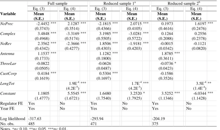
Looking at the results from the full sample first, both Complex and NoRev have negative coefficient estimates in (4), implying that more complex cases and regulatory experience lead to lower effort. The coefficients of NoPrec and LengTot also have the expected signs in (4) as more precedents reduce the
19 In a preliminary specification we also included the interaction of Complex and NoRev, but that model did not converge.
17 cost of effort and higher absolute prices make the regulator more concerned about protecting
consumers. Estimates in (3) are also broadly consistent with expectations. More precedents mean that more information is available, reducing the review time and complexity and experience increase the review time. This last result is consistent with the regulator gradually encountering further
complexities as she gains more experience.
Table 3. Parameter estimates for regulator effort, i.e. equations (3) and (4).
Full sample Reduced sample 1a Reduced sample 2b Eq. (3) Eq. (4) Eq. (3) Eq. (4) Eq. (3) Eq. (4)
Variable Mean (S.E.) Mean (S.E.) Mean (S.E.) Mean (S.E.) Mean (S.E.) Mean (S.E.) NoPrec -2.4452 (0.3743) *** 2.1287 (0.3514) *** -2.1815 (0.4366) *** 2.0715 (0.4105) *** 0.1973 (0.4616) 1.6197 (0.2476) *** Complex 3.4848 (0.4968) *** -3.3169 (0.5174) *** 3.1985 (0.5505) *** -3.0281 (0.5722) *** 0.1264 (0.2088) 0.2556 (0.2378) NoRev 2.3562 (0.4342) *** -2.3666 (0.4277) *** 1.8506 (0.4303) *** -1.9181 (0.4203) *** -0.0015 (0.0342) -0.1121 (0.0820) Antenna 1.1537 (0.1733) *** 1.1282 (0.1800) *** 1.8785 (0.3611) *** ThreeLar -0.0822 (0.0505) -0.0626 (0.0487) -0.0736 (0.0423) * CustCorp 0.4184 (0.1619) *** 0.5304 (0.1697) *** -0.1586 (0.3526) LengTot 1.9E-4 (4.2E-5) *** 1.7E-4 (4.2E-5) *** 3.5E-4 (1.4E-4) ** Constant 1.1805 (1.4777) 5.5545 (1.6721) *** 1.6480 (1.7540) 3.2520 (1.7925) * 3.5252 (1.1346) *** -6.0344 (1.1428) ***
Regulator FE Yes No Yes No Yes No
Year FE Yes No Yes No Yes No
Log likelihood -317.63 -293.94 -204.19
No. obs. 485 471 375
Notes. *p< 0.10, **p< 0.05, ***p< 0.01.
a
Observations excluded: (i) Incidental regulators, i.e. regulators who have chaired only one or two connection reviews in total; and (ii) Regulatory decisions made before 2006.
b
Observations excluded: as in ‘Reduced sample 1’, and in addition: (iii) observations when regulator has chaired more than 200 decisions.
The estimates based on the sample where incidental regulators and decisions made before 2006 are excluded (Reduced sample 1) are practically identical to the ones for the full sample. The estimates change markedly when using the sample where regulators who chaired more than 200 decisions are also excluded (Reduced sample 2). Several of the coefficients change sign and some that had no significant impact are now highly significant. The previous estimates, that are largely consistent with expectations, have been replaced with outcomes that seem much less plausible. It is likely that reducing the sample this much has not made it possible for the simultaneous equations to identify the
18 true underlying data generating process and thus, we do not pay any detailed attention to these results. Overall, we are therefore inclined to conclude that both complexity and regulatory experience are negatively related to effort.
4.2 Regulator’s price setting
In this section we investigate how the regulator adjusts the price claimed by the utility. Hence, the
dependent variable of interest can be written as U
R
P
P . Taking the ratio of these two prices has the
advantage of eliminating the influence of any basic cost drivers, such as transformers and the amount of power, for which the regulator has long since established templates that are accepted by the utilities.
According to predictions (iii)-(v) at the end of Section 2, the regulator’s price level will be determined by the number of chaired reviews (NoRev), case complexity (Complex) and their interactions
(NoRev Complex). As controls we add the number of precedents (NoPrec), line length above 560 meters (Leng560) and case, utility and customer characteristics (Antenna, ThreeLar and CustCorp). Regulator and time fixed effects are included. Hence, the model that explains the regulator’s price setting is formulated as:
(6)
where notations are as in (1). As before we test the sensitiveness of excluding observations that might not be representative. However, the potentially most serious problem when estimating (5) is that NoRev is endogenous. That can happen if regulators who set lower prices are more likely to stay longer as chairs. That was exactly what Smyth and Söderberg (2010) found in their analysis of the rotation of regulators in the Swedish electricity market. Their explanation was that DGs have adopted policies consistent with the intent of the market reform, which was to protect the consumers. However, since about 2005 the Director Generals have not used the policy of rotating regulators that was used in the period after the market deregulation (1996-2004). In recent years the regulators have been more independent and chaired relatively large numbers of consecutive decisions. The position as chair for customer disputes has tended to be associated with the position as departmental manager for customer disputes, a position that the individual keeps for as long as s/he likes. However, in principle it cannot be ruled out that the DG influences the appointment of regulators. To control for this potential
19 endogeneity we use share of decisions made in favour of customers (both in level and squared) and share of decisions appealed as instruments for NoRev in one of the estimations. Share of decisions in favour of customers was the variable that Smyth and Söderberg (2010) suggested had an impact on the number of decisions chaired by regulators. With more data than Smyth and Soderberg, we find that share of decisions being appealed is also a relevant instrument. The first stage F-statistic for NoRev using these instruments is 5.35, which passes the common rule of thumb at 5 commonly used in the literature.
Results presented in Table 4 are reasonably robust across samples. Moreover, while the IV-model gives results that are generally consistent with the other models, the endogeneity test shows that NoRev can be treated as exogenous.20 These two findings suggest that regulators generally raise the price as cases get more complex and that they lower the price as they get more experienced. While not statistically significant, one can also observe that the interaction between the two factors is positive, resulting in experienced regulators responding more strongly to complexity, i.e. they increase the price at a faster rate when complexity increases.
20 The endogeneity test is calculated as the difference of two Sargan-Hansen statistics: one for the equation where NoRev is treated as endogenous, and one for the equation where NoRev is treated as exogenous.
20
Table 4. Parameter estimates for regulator’s price setting, i.e. equation (6).
Full sample Full sample,†NoRev endogenous Reduced sample 1 a Reduced sample 2 b Variable Coeff. (S.E.) Coeff. (S.E.) Coeff. (S.E.) Coeff. (S.E.) NoRev -3.2E-4 (1.2E-4) ** -0.0020 (0.0019) -3.3E-4 (1.1E-4) ** -3.0E-4 (2.0E-4) Complex 0.0238 (0.0107 * -0.0286 (0.0636) 0.0240 (0.0109) * 0.0272 (0.0101) *
NoRev Complex 1.5E-4
(1.6E-4) 0.0011 (0.0011) 1.5E-4 (1.6E-4) 4.3E-5 (1.2E-4) NoPrec 0.0017 (2.9E-4) *** 0.0026 (0.0012) ** 0.0018 (3.3E-4) *** 9.8E-4 (0.0065) Leng560 0.1406 (0.0255) *** 0.1356 (0.0257) *** 0.1403 (0.0269) *** 0.1490 (0.0322) *** Antenna -0.1019 (0.0162) *** -0.0637 (0.0890) -0.0925 (0.0189) *** -0.0532 (0.0374) ThreeLar -0.0045 (0.0200) 0.0105 (0.0306) -0.0025 (0.0207) -0.0307 (0.0300) CustCorp 0.0805 (0.0109) *** 0.0298 (0.0948) 0.0789 (0.0117) *** 0.0413 (0.0315)
Regulator FE Yes Yes Yes Yes
Year FE Yes Yes Yes Yes
Hansen J, P-value 0.169
Endogeneity test, P-value
0.245
First stage F-statistic for NoRev
5.35
R2 0.126 0.074 0.112 0.115
No. of obs. 489 486 475 376
Notes. *p< 0.10, **p< 0.05, ***p< 0.01. S.E. are clustered over regulators; 7 in the full sample and 5 when samples are reduced.
† Incidental regulators, i.e. regulators who have chaired only one or two connection reviews in total, are excluded.
a
Observations excluded: (i) Incidental regulators, i.e. regulators who have chaired only one or two connection reviews in total; and (ii) Regulatory decisions made before 2006.
b Observations excluded: as in ‘Reduced sample 1’ and in addition: (iii) observations when regulator has chaired more than 200 decisions.
4.3 Court’s price setting
As in section 4.2 to eliminate basic cost drivers, we use the ratio of the amount awarded by the court ( C
P ) and the regulator (PR) as our dependent variable. Based on the investigation in Section2, we specify the court’s price setting in the same way as the regulator’s price setting. Hence, we can write:
21
, (7)
where notations are as in (6). Estimates of (7) are displayed in Table 5, but before taking a closer look at these results we consider the potential problem that appealed cases might not constitute a random sample of complaints. In addition to the estimates presented in Table 5, we therefore estimate a selection model (Heckman-model estimated with ML) using NoRev, Complex and LengLow as explanatory variables in the selection model, but there is no evidence of the appealed sub-sample being non-random.21
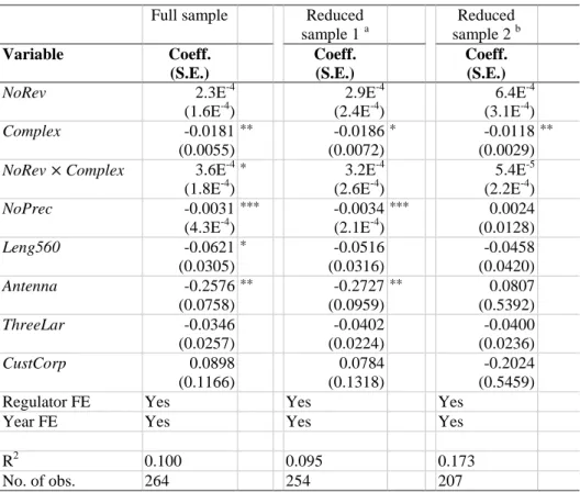
Table 5. Parameter estimates for court’s price setting, i.e. equation (7).
Full sample Reduced sample 1 a Reduced sample 2 b Variable Coeff. (S.E.) Coeff. (S.E.) Coeff. (S.E.) NoRev 2.3E-4 (1.6E-4) 2.9E-4 (2.4E-4) 6.4E-4 (3.1E-4) Complex -0.0181 (0.0055) ** -0.0186 (0.0072) * -0.0118 (0.0029) **
NoRev Complex 3.6E-4
(1.8E-4) * 3.2E-4 (2.6E-4) 5.4E-5 (2.2E-4) NoPrec -0.0031 (4.3E-4) *** -0.0034 (2.1E-4) *** 0.0024 (0.0128) Leng560 -0.0621 (0.0305) * -0.0516 (0.0316) -0.0458 (0.0420) Antenna -0.2576 (0.0758) ** -0.2727 (0.0959) ** 0.0807 (0.5392) ThreeLar -0.0346 (0.0257) -0.0402 (0.0224) -0.0400 (0.0236) CustCorp 0.0898 (0.1166) 0.0784 (0.1318) -0.2024 (0.5459)
Regulator FE Yes Yes Yes
Year FE Yes Yes Yes
R2 0.100 0.095 0.173
No. of obs. 264 254 207
Notes. *p< 0.10, **p< 0.05, ***p< 0.01. S.E. are clustered over regulators; 7 in the full sample and 5 when samples are reduced.
a Observations excluded: (i) Incidental regulators, i.e. regulators who have chaired only one or two connection reviews in total; and (ii) Regulatory decisions made before 2006.
b
Observations excluded: as in ‘Reduced sample 1’, and in addition: (iii) observations when regulator has chaired more than 200 decisions.
22 In Table 5 one can observe that NoRev is positive, but not statistically significant; Complex is negative and generally significant at conventional levels, and the interaction between NoRev and Complex is positive and significant when the full sample is used. These marginal effects are consistent with predictions (vi)-(viii) but we evaluate them more formally in the next section (4.4).
4.4 Consistency between theory and evidence
In this section we calculate predicted values of (6) and (7) for different types of regulators and levels of case complexity. As displayed in Table A1, NoRev ranges from 1 to 306 and Complex from 1 to 11. For the purpose of calculating predicted values, we set number of chaired decisions (NoRev) to 20 to represent a regulator who only cares about his career and to 100 to represent a regulator who cares
about both his career and consumer surplus.22 Next we tabulate the predictions of and based on (6) and (7) using the full samples, for the two experience levels when { }, where low (high) levels represent relatively uncomplicated (complicated) cases. The results of these
predictions are shown in Table 6.
Table 6. Price-setting by the regulators and the court. Complexity ⁄ when
regulator only cares about his
career
⁄ when regulator cares
about both his career and CS
⁄ when regulator only cares
about his career
⁄ when regulator cares
about both his career and CS 1 0.7124 (0.0051) 0.6983 (0.0005) 0.9888 (0.0067) 1.0360 (0.0020) 3 0.7660 (0.0198) 0.7756 (0.0118) 0.9672 (0.0116) 1.0720 (0.0273) 5 0.8196 (0.0348) 0.8530 (0.0240) 0.9455 (0.0180) 1.1080 (0.0567) 7 0.8732 (0.0498) 0.9303 (0.0362) 0.9238 (0.0248) 1.1440 (0.0860) 9 0.9268 (0.0649) 1.0076 (0.0484) 0.9021 (0.0317) 1.1800 (0.1153) Notes: Standard errors in brackets. Results are calculated when regulator who only cares about his career is defined as having chaired 20 decisions, and a regulator who cares about both his career and consumer surplus is defined as having chaired 100 decisions.
23 Prediction (iii) states that regulators set lower prices when cases are uncomplicated. Our results for both types of regulators are indeed consistent with this prediction. Predictions (iv) and (v) say that regulators who care about both their careers and consumer surplus set lower prices and respond more strongly to complexity (i.e. they increase the price at a higher rate as complexity increases) than those who only care about their career. These predictions are confirmed except for medium and high levels of complexity when career oriented regulators set higher prices. Predictions (vi)-(viii) postulate that the court reduces the regulator’s decision when she is strictly career oriented and that the court sets the same (higher) price as the regulator when the case is uncomplicated (complicated) when she cares about both her career and consumer surplus. These predictions are confirmed empirically.
5. CONCLUSIONS
Leaver (2009) provides a theoretical framework and convincing empirical evidence showing that the length of office terms for regulators is negatively related to both the probability of initiating regulatory reviews and regulated prices. Shorter office terms are associated with more substantive career
concerns by regulators – after all, the shorter the term the more immediate will be the concerns of a regulator with her career and finding her next job. A regulator with career concerns can bias her decisions to favour firms if she is interested in an industry job, or consumers if she is interested in being reappointed. Therefore, Leaver (2009) can be seen as presenting a powerful case for longer office terms for regulators.
This paper provides some powerful empirical evidence, based on a number of predictions derived from a model of regulatory behaviour, suggesting that one cannot take Leaver’s conclusion to its limit. That is, a very long term office (e.g. life tenure) brings its own distortions to regulatory decision making which arises from the interplay between the regulator’s experience, the level of complexity of the regulatory decision, the choice of effort by the regulator and the impact of explicit external evaluation on a regulator’s career prospects.
In particular, when the regulator is only concerned about her career, as a more inexperienced regulator who might be concerned with securing her current job or being promoted within the public service, we show that a larger number of decisions will be overturned by the court when cases are more complex than in situations in which the case is less complex. We also show that when the regulator cares about both her career and consumer surplus, as a more experienced regulator might do, less complex cases will be associated with more appeals by regulated firms, but fewer decisions will be overturned and
24 prices will be lower. As the complexity of the case increases, we predict a switch to more appeals by consumers, more decisions being overturned and higher prices on average. Moreover, regulators who care about both their careers and consumer surplus will exert less effort when cases become more complex. By and large, these predictions are borne by our empirical analysis.
REFERENCES
Breunig, R. and F. M. Menezes (2012), Testing regulatory consistency, Contemporary Economic Policy, Vol. 30, Issue 1, pp. 60–74.
Breunig, R., J. Hornby, F. M. Menezes and S. Stacey (2006). Price regulation in Australia: how consistent has it been? Economic Record, Vol. 82, No. 256, pp. 67–76.
Camerer, C. and K. Weigelt (1988), Experimental tests of a sequential equilibrium reputation model, Econometrica 56(1), pp. 1-36.
Clermont, K. and Eisenberg, T. (2002), Plaintiphobia in the appellate courts: civil rights really do differ from negotiable instruments?, University of Illinois Law Review, Vol. 2002, pp. 947–978.
Davis, L.W. and Muehlegger, E. (2010), Do Americans consume too little natural gas? An empirical test of marginal cost pricing, RAND Journal of Economics, Vol. 41, No. 4, pp. 791–810.
DeFigueiredo, R. and Edwards, G. (2007), Does private money buy public policy?: campaign
contributions and regulatory outcomes in telecommunications, Journal of Economics and Management Strategy, Vol. 16, No. 3, pp. 547–576.
Garside, L., Grout, P.A. and Zalewska, A., (2013), Does experience make you ‘tougher’? Evidence from competition law, Economic Journal, Vol. 123, No. 568, pp. 474-490.
Gennaioli, N. and Shleifer, A. (2008), Judicial Fact Discretion, Journal of Legal Studies Vol. 37, No. 1, pp. 1-35.
Glaeser, E. L. and Shleifer, A. (2003), The Rise of the Regulatory Sate, Journal of Economic Literature Vol. 41, No 2, pp. 401-425.
Jordana, J., Levi-Faur, D., Marín, X.F. (2011), The global diffusion of regulatory agencies: channels of transfer and stages of diffusion, Comparative Political Studies, Vol. 44, No.10, pp. 1343–1369.
Kaheny E.B., Haire S.B. and Benesh S.C. (2008), Change over tenure: voting, variance and decision making on the US courts of appeals, American Journal of Political Science, Vol. 52, No. 3, pp. 490– 503.
Knittel, C. (2003), Market structure and the pricing of electricity and natural gas, Journal of Industrial Economics, Vol. 51, No. 2, pp. 167–191.
Leaver, C. (2009), Bureaucratic minimal squawk behaviour: theory and evidence from regulatory agencies, American Economic Review, Vol. 99, No. 3, pp. 572–607.
25 Niskanen, W.A. (1971), Bureaucracy and representative government, Aldine, New York.
Prendergast, C. (2007), The motivation and bias of bureaucrats, American Economic Review, Vol. 97, No. 1, pp. 180–196.
Prendergast, C. (2003), The limits of bureaucratic efficiency, Journal of Political Economy, Vol. 111, No. 5, pp. 929–958.
Priest, G.L. and Klein, B. (1984), The selection of disputes for litigation, Journal of Legal Studies, Vol. 13, No. 1, pp. 1–55.
Shavell, S. (2004), The appeals process and adjudicator incentives, NBER Working Paper 10754.
Shavell, S. (1995), The appeals process as a means of error correction, Journal of Legal Studies, Vol. 24, pp. 379–426.
Shleifer, A., (2012), The Failure of Judges and the Rise of Regulators, MIT Press, Cambridge, Massachusetts.
Silva, H.C.D. (2011), Cost efficiency in periodic tariff reviews: the reference utility approach and the role of interest groups, Mimeo.
Smyth, R. and Söderberg, M. (2010), Public interest versus regulatory capture in the Swedish electricity market, Journal of Regulatory Economics, Vol. 38, No. 3, pp. 292–312.
Stigler, G.J. (1971), The theory of economic regulation, Bell Journal of Economics & Management Science, Vol. 2, pp. 3–21.
Wilson, R. (1985), Reputations in Games and Markets, in Game-theoretic Models of Bargaining, ed. by A. E. Roth. Cambridge: Cambridge University Press.
26
Appendix 1
Proof of Proposition 1
First, we calculate the regulator’s expected utility conditional on effort. Then, we determine the optimal level of effort and the associated regulated price. For E , the regulator fully uncovers the regulated firm’s true cost. In this case, if the regulator uncovers cH, and sets the regulated price pR
equal to cH, then they obtain utility:
p c E c
U U R H | , H .
In this case, the consumer appeals to the court with probability . However, the court does not reverse the regulator’s decision. If instead the regulator sets pR cL, they obtain utility:
p c E c
U U R L| , H ( ) (1 ) .
In this case, the regulated firm appeals to the court with probability and the court reverses the decision. Note that U
pRcH |E,cH
U pRcL|E,cH
. If instead, the regulator uncovers cL, then their utility under the two possible prices is equal to:
p c E c
U U R H | , L ( ) (1 ) and
p c E c
U U R L| , L . Note that U
pR cL|E,cL
U pR cH |E,cL
.We now look at the case where the regulator chooses E 0 and, as such, does not know the true realised costs and so computes their expected utility as follows:
p c E
qU q
U
27 and
p c E
qU q
U
U R L| 0 (1 ) ()(1) .
Note that U
pR cL|E0
U pR cH |E0
if 1qq
.Finally, note that for
q q
1 , the regulator chooses effort E 0 if
q q
qU U (1 )(1 ) (1 ) .
That is, the regulator chooses E 0 and pR cH when
q q 1 and
(1
q
) (
U
)
. ■ Proof of Proposition 3.For E, we can calculate the regulator’s expected utility when cH is realised as follows:
p c E c
U UCS R H | , H and
R L| , H
()(1)( H L) CS p c E c U c c U . Note that UCS
pR cH |E,cH
UCS
pR cL|E,cH
if 1 (cH cL) U
.28 This inequality holds, for example, whenever the probability that the regulated high cost firm appeals
following a regulatory decision where pR cL is sufficiently close to one. Conversely, the inequality is unlikely to hold if is small or if the consumer’s surplus is large.
Similarly, if is realised, then the regulator’s expected utility is given by:
| , ( ( )) (1 )( )
CS R
H L H L
U p c E
c
c c
U
.That is, in this case, the consumer appeals to the court with probability and the court overturns the regulator’s decision and the price reduces to cL. Similarly,
p c E c
c c U UCS R L| , L ( H L) .
Note that if the regulator chooses E, then they will set pR cLwhen the utility is of a low cost type.
We now consider the case where E0 and compute the regulator’s expected utility as follows:
p c E
qU q
c c U
UCS R H | 0 (1 )(( H L))(1) and
R L| 0
( ) (1 )
(1 )
( H L)
CS p c E q U q U c c U .When E 0, the regulator sets pR cH whenever
q
q
c
c
q
U
H L
)
1
(
)
)(
1
)(
1
(
(A1)29 and this inequality holds as long as
q q
1 . (Since we need the denominator to be positive so that the
sign won’t change when we divide the inequality by it). Finally, whenever (A1) is satisfied, the regulator will choose effort