HAL Id: hal-03208423
https://hal.archives-ouvertes.fr/hal-03208423v2
Submitted on 29 Apr 2021
HAL is a multi-disciplinary open access
archive for the deposit and dissemination of
sci-entific research documents, whether they are
pub-lished or not. The documents may come from
teaching and research institutions in France or
abroad, or from public or private research centers.
L’archive ouverte pluridisciplinaire HAL, est
destinée au dépôt et à la diffusion de documents
scientifiques de niveau recherche, publiés ou non,
émanant des établissements d’enseignement et de
recherche français ou étrangers, des laboratoires
publics ou privés.
DECA: a Dynamic Energy cost and Carbon
emission-efficient Application placement method for
Edge Clouds
Ehsan Ahvar, Shohreh Ahvar, Zoltan Adam Mann, Noel Crespi, Joaquin
Garcia-Alfaro, Roch Glitho
To cite this version:
Ehsan Ahvar, Shohreh Ahvar, Zoltan Adam Mann, Noel Crespi, Joaquin Garcia-Alfaro, et al.. DECA:
a Dynamic Energy cost and Carbon emission-efficient Application placement method for Edge Clouds.
IEEE Access, IEEE, In press, pp.1-23. �10.1109/ACCESS.2021.3075973�. �hal-03208423v2�
***Authors (draft) version***
*This paper has been accepted in IEEE Access*
D-CACEV: a Dynamic Cost and Carbon
Emission-Efficient Virtual Machine Placement
Method for Green Distributed Clouds
Ehsan Ahvar, Shohreh Ahvar, Zoltan Adam Mann,
Noel Crespi, Joaquin Garcia-Alfaro, and Roch Glitho,
Abstract—As an increasing amount of data processing is done at the network edge, high energy costs and carbon emission of Edge
Clouds (ECs) are becoming significant challenges. The placement of application components (e.g., in the form of containerized microservices) on ECs has an important effect on the energy consumption of ECs, impacting both energy costs and carbon emissions. Due to the geographic distribution of ECs, there is a variety of resources, energy prices and carbon emission rates to consider, which makes optimizing the placement of applications for cost and carbon efficiency even more challenging than in centralized clouds. This paper presents a Dynamic Energy cost and Carbon emission-efficient Application placement method (DECA) for green ECs. DECA addresses both the initial placement of applications on ECs and the re-optimization of the placement using migrations. DECA considers geographically varying energy prices and carbon emission rates as well as optimizing the usage of both network and computing resources at the same time. By combining a prediction-based A* algorithm with Fuzzy Sets technique, DECA makes intelligent decisions to optimize energy cost and carbon emissions. Simulation results show the applicability and performance of DECA.
Index Terms—Edge cloud, Energy consumption, Energy costs, Green computing, Carbon emission, Application placement.
F
1
I
NTRODUCTIONThe Internet of Things (IoT) is producing rapidly increasing amounts of data. Data analytics applications that process IoT data require significant computational capacity, which IoT devices typically do not possess. Using centralized cloud data centers to host the analytics applications is an option, but transferring the data from the IoT devices to the cloud incurs high latency and large network traffic. Therefore, new distributed computing paradigms that move processing closer to the network edge (fog computing, edge computing etc.) are gaining popularity. In the computing model considered in this paper, computational resources are provided in several Edge clouds (ECs) instead of a single centralized cloud. ECs have limited capacity and are geographically distributed. Applications can be deployed on ECs, and data produced by IoT devices can be processed in an EC near the IoT devices. Thereby, latency and network traffic are significantly reduced, making ECs an attractive paradigm for many IoT applications [1], [2].
E. Ahvar is with Learning, Data and Robotics Lab, ESIEA, Paris, France. e-mail: ([email protected]).
S. Ahvar is with ISEP-Institut Sup´erieur d’ ´Electronique de Paris. e-mail: ([email protected]).
N. Crespi, J. Garcia-alfaro are with T´el´ecom SudParis, Institut Polytech-nique de Paris, France. e-mail: (noel.crespi, joaquin.garcia [email protected]).
Z. A. Mann is with University of Duisburg-Essen, Germany. e-mail: ([email protected]).
R. Glitho is with Concordia University, Canada. e-mail: ([email protected]).
With the rise of data processing in ECs, the increasing energy consumption of ECs is becoming a major concern for two reasons: energy costs and carbon emissions. Both energy costs and carbon emissions are becoming pressing issues for the providers of ECs [10].
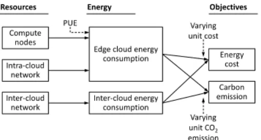
Similar to centralized clouds, also ECs need energy saving methods, e.g., workload consolidation. However, minimizing en-ergy costs and carbon emissions in ECs is a more complex problem. Energy prices and carbon emission rates vary by location and even by time (e.g., because of different local energy sources). Therefore, even the same energy consumption may lead to differ-ent energy costs and carbon emissions depending on which EC (and when) serves the given workload. It is important to note that there is no correlation between the cleanness (carbon footprint) and the price of a location’s energy sources [3]. Hence, optimizing energy costs and carbon emissions are two independent objectives. We consider an infrastructure comprising several geographi-cally distributed ECs, where each EC consists of a set of Compute Nodes (CNs). A set of applications is to be placed on this infrastructure. Every application consists of one or more com-ponents, for example in the form of containerized microservices. For every component, detecting an appropriate place (in which of the ECs, on which CN) is considered as an important issue. For the component placement, there is a variety of resources, energy prices and carbon emission rates to consider. To optimize energy costs and carbon emissions, we have three levers: (i) minimizing energy consumption (usually by optimizing resource utilization), (ii) choosing resources in locations with low energy price, and
DECA
DECA: a Dynamic Energy cost and Carbon emission-efficient
Application placement method for Edge Clouds
Resources Compute nodes Intra-cloud network Inter-cloud network Energy
Edge cloud energy consumption Inter-cloud energy consumption Objectives Energy cost Carbon emission PUE Varying unit cost Varying unit CO2 emission
Fig. 1. Sources of energy consumption and its impact on optimization objectives
(iii) choosing resources in locations with low carbon emission rate. Hence the challenge is to consider these three, sometimes conflicting aims simultaneously (see also Fig. 1).
To address the above problem, this paper proposes a dynamic energy cost and carbon emission-efficient application placement method (DECA) for ECs, considering the above three levers to optimize both energy costs and carbon emissions in distributed ECs. DECA includes two main parts: (i) determining the initial placement of newly deployed applications and (ii) re-optimization of the placement of applications to react to workload changes. In contrast to most previous works, DECA considers both CNs and network devices because both of them may contribute significantly to energy consumption.
DECA combines a variant of the A* search algorithm [6] with a Fuzzy Sets technique [7]. Using these powerful techniques, DECA can perform more effective optimization than traditional greedy heuristics used by most existing approaches [8], [9]. We describe in the Appendix the benefit of the A* algorithm for application placement in ECs compared to other heuristics.
DECA performs joint optimization of compute and network resources, also considering their associated energy price and carbon emission rate. It can select CNs from multiple ECs to place the components of an application, in order to (i) be able to achieve low overall energy cost and carbon emission and (ii) overcome capacity limitations of a single EC.
Our major contributions are summarized below:
1) We build this work based on our previous work on green
cloud computing [10], adapting it to the characteristics of emerging EC systems and improving its application placement method (i.e., from static placement to dy-namic).
2) To offer a better view about DECA mechanism, a
com-prehensive logical architecture is presented.
3) New methods for the dynamic re-optimization of the
placement using live migration are proposed. Two AC migration mechanisms are proposed for under-utilized and over-utilized CNs respectively.
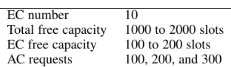
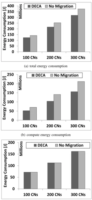
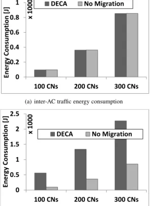
4) We perform a comprehensive comparison on energy cost,
carbon footprint and energy consumption for different AC placement algorithms.
The rest of the paper is organized as follows. Section 2 describes related work. Section 3 introduces our problem for-mulation. Section 4 provides the algorithmic solution underlying DECA. Section 5 evaluates DECA. Section 6 concludes the paper.
2
R
ELATED WORKAs already mentioned, the applications are assumed to be made of independently deployable ACs, for example in the form of VM-based or containerized microservices. The provider should make a decision on resource allocation for the components by selecting the most suitable CN. This process is known as placement.
In recent years, many different aspects of the placement prob-lem (mostly in the form of VM placement) have been investigated [9]. We can divide the related work into three categories: i) the works which focus on improving energy consumption and cost, ii) the studies which consider both energy consumption/cost and carbon emission together, iii) the works that utilize AC or VM migration algorithms to improve energy consumption and/or carbon emission.
2.1 Energy consumption and cost
Li et al. [11] considered network and compute resources at the same time for their allocation algorithm. Pahlevan et al. [12] proposed an energy- and network-aware approach that integrates heuristic and machine learning methods. You et al. [13] designed a network-aware VM placement method to improve communication cost. Although these works considered also the optimization of data transfer, they are limited to a single-node (i.e., centralized cloud) environment and are not appropriate for a distributed EC with varying resource prices and carbon emission rates.
Goudarzi et al. [47] have recently proposed an application placement technique based on the Memetic Algorithm to make batch application placement decision for IoT applications in a heterogeneous Edge and Fog computing environment. However, in this work, the energy consumption is considered from the IoT device perspective. They also do not consider the price of energy. Pallewatta et al. [48] proposed a microservices-based IoT application placement technique for heterogeneous and resource constrained fog environments. They also proposed a fog node architecture to support their proposed placement approach. But their main objective is to minimize latency and network usage, and not energy costs.
Hu et al. [49] proposed an approach to optimize the placement of service-based applications in clouds for reducing the inter-machine traffic. They first partition the application into several parts while trying to keep the overall traffic between the created parts to a minimum. Then, the created parts are carefully located into machines with respect to their resource and traffic demands. However, they do not consider energy cost optimisation.
Hassan et al. [50] have recently proposed a method for service placement in fog-cloud systems. They classified services into two categories: critical and normal ones. For critical services, they try to minimize response time, and for normal ones the goal is to reduce the energy consumption of the fog environment.
The same authors [52] formulated the VM placement of IoT
applications in Cloud DCs as an MILP model and proposed two algorithms. Minimization of the power (i.e., CPU) and network for the first algorithm. And second algorithm focuses on reducing the power (i.e., CPU) and resources wastage. Yet, carbon emission and energy cost optimisation has not been accounted for in these two works.
Kayal et al. [51] proposed a placement strategy to jointly opti-mize energy consumption of fog nodes and communication costs of applications. The algorithm applies the Markov approximation
method to solve the combinatorial optimization objective. How-ever, they are concerned with methods for assigning microservices to fog nodes with the objective of balancing energy consumption at fog nodes and network traffic costs.
Nabavi et al. [53] proposed a multi-objective VM placement scheme (considering VMs as fog tasks) for edge cloud DCs called TRACTOR using an artificial bee colony optimization algorithm. TRACTOR goal is power and network-aware assignment of VMs onto PMs. The proposed scheme aims to minimize the network traffic of the interacting VMs and the power dissipation of the DC’s switches and PMs.
Our current work is different from all above-mentioned results since we consider not only energy costs but also carbon emission.
2.2 Both energy consumption (cost) and carbon emis-sion
Khosravi et al. [16] considered both carbon emission and energy during VM allocation. However, they did not consider the variabil-ity of energy prices. Also, inter-VM (inter-AC) communication was not considered, although it is an important factor for reducing energy of network resources. Khosravi et al. in [17] have presented several energy and carbon-aware algorithms. But they did not consider the energy consumed by network elements in their energy model. Zhou et al. [4] jointly considered electricity cost, emission and Service Level Agreement (SLA) reduction for distributed ECs, while Gu et al. [18] presented a method to minimize carbon emission of ECs or Data Centers (DCs) while satisfying constraints on response time, electricity budget and maximum number of running CNs in an environment with homogeneous CNs. These papers target service jobs with constraints on response time. Moreover, different from all mentioned works, our work considers both component (VM) placement and migration to keep costs and emissions low.
2.3 AC (VM) migration
Tziritas et al. [19] targeted the problem of placement considering two objectives: (1) to minimize energy consumption of the CNs, and (2) to minimize the network overhead stemming from commu-nication between VMs and from VM migrations. They select the most energy-consuming CN based on both maximum power and current workload to migrate its VMs. This method may select CNs with low power consumption but heavy workload as migration source and CNs with high power consumption and low workload as destination, which may lead to sub-optimal results.
Zhou et al. [20] proposed a VM deployment algorithm called three-threshold energy saving algorithm (TESA) and five VM selection algorithms: MIMT, MAMT, HPGT, LPGT and RCT. Unlike our work which selects a destination CN based on both communication and compute resource metrics, they select a CN with the least increase of power consumption (we called it Min. Compute policy) due to VM allocation. This way, the target CN may be located far from the source CN so that migration consumes a large amount of energy.
Mustafa et al. [30] proposed two consolidation based tech-niques to reduce energy consumption along with resultant SLA violations. They also enhanced two existing techniques that at-tempt to reduce energy consumption and SLA violations. They finally show that the proposed techniques perform better than the selected heuristic based techniques in terms of energy, SLA, and migrations.
Zheng et al. [21] proposed a dynamic energy efficient resource allocation scheme. They consider a mapping probability matrix where each VM request is assigned with a probability on a specific CN. The proposed method then decides where to allocate new VM requests and whether to migrate existing VMs in order to improve energy efficiency. Although the authors proposed an idea to migrate VMs for energy reduction, their exact solution in situation of CN overloading is not clear.
Beloglazov et al. [22] devised heuristics to continuously con-solidate VMs leveraging live migration and switching off idle CNs to minimize the number of utilized CNs. They proposed a modified version of the Best Fit Decreasing algorithm (MBFD) to place VMs on CNs and four heuristics to select VMs for migration. They did not consider the energy consumption of network elements. In another study, Beloglazov et al. [23] proposed three stages of VM placement optimization including reallocation based on current utilization of multiple system resources, optimization of virtual network topologies established between VMs and VM reallocation considering thermal state of the resources. However, Beloglazov et al. in both studies did not consider carbon emission.
Liu et al. [24] developed an ant colony system-based approach to reduce cloud energy consumption. To handle both homogeneous and heterogeneous CN environments, they also proposed an order exchange and migration mechanism. However, their objective is limited to minimizing the number of active CNs. Forestiero et al. [25] proposed a hierarchical method (i.e, composed of two workload assignment and migration algorithms) for efficient workload management in distributed ECs. Li et al. [26] proposed a dynamic virtual machine scheduling algorithm, called GRANITE, to minimize total EC energy consumption. However, these works do not take into account carbon emission.
Ibrahim et al. [54] attempted to reduce consumed energy, number of VM migrations, number of host shutdowns and the combined metric Energy SLA Violation (ESV) with a dynamic consolidation of VMs. In the method, the servers are checked peri-odically and appropriate VMs from under and over utilised servers are migrated to destinations selected based on Particle Swarm Optimization techniques. The authors mentioned that increasing energy consumption has a significant impact on the environment due to emissions of carbon. However, they have not done any study in carbon emission reduction. Cost also was not considered by the authors.
Table 1 lists the related works considering their main objec-tives/characteristics. All mentioned related works addressed some of the points listed in the Introduction to characterize the problem, but only in isolation, missing some other important aspects. Our previous work CACEV [10] is the first to address most aspects in combination, although in a cloud computing setting. It is also the first VM placement algorithm integrating the prediction-based A* search algorithm [6] with a Fuzzy Sets technique [7]. However, CACEV makes only a static VM placement. Our current work, DECA, extends CACEV to ECs and with support for VM migrations. Different from related works on VM consolidation, DECA uses a fuzzy set-based decision maker which can sharply improve its performance.
3
P
ROBLEM FORMULATION3.1 System model
To offer a realistic solution, the paper considers a system model characterized by the following points:
TABLE 1 Related Work Summary
Reference energy saving/cost carbon emission AC/VM migration
[11], [12], [13], [47], [48], [49], [50], [51], [52], [53] X
[4], [16], [17], [18] X X
[19], [20], [21], [22], [23], [24], [25], [26], [54] X X
1) Heterogeneity of ECs, CNs, and network devices in terms
of capacity and energy consumption characteristics.
2) Heterogeneity of application components in terms of
resource needs.
3) Load-dependent energy consumption (for example, the
energy consumption of a CN depends on its CPU load).
4) Joint optimization of compute and network resources.
5) Arbitrary network topology among ECs and within ECs;
in particular, there can be multiple network paths between a pair of CNs.
6) Variety in unit energy price and unit carbon footprint
among ECs.
7) Ability to select CNs from multiple ECs to place the
components of an application.
8) Taking into account the communication between
applica-tion components and the associated impact on network traffic, preferring to place components with intensive communication close to each other.
9) Workload consolidation by live migration of application
components.
We consider a hierarchical distributed architecture [27] consisting of a set of ECs, with each EC consisting of a set of CNs. The ECs and the inter-cloud connectivity information are given by a graph
𝐺0= (𝐷, 𝐸, 𝑤𝐷, 𝑤𝐸) where 𝐷 is the set of ECs, 𝑤𝐷 denotes their
current capacity, 𝐸 consists of connections (network paths) among the ECs, and 𝑤𝐸 denotes the weights of the connections (e.g., number of routers on the network paths). Each EC is characterized by a Power Usage Effectiveness (PUE) value and is associated with one or more energy sources with different energy prices and carbon footprint rates. PUE is considered as the ratio of total power consumed by the EC to the power consumed by IT devices within the EC [16]. We assume a high-capacity backbone network to carry the traffic between the ECs. Inside an EC, the model (and our proposed algorithm) supports both structured (e.g., Fat-Tree [38]) and arbitrary [28] topologies. Table 2 gives an overview of the abbreviations and notations used in the paper.
Each EC 𝑑 ∈ 𝐷 is represented by a weighted graph 𝐺𝑑 =
(𝑁𝑑, 𝐸𝑑, 𝑤 𝑁𝑑, 𝑤 𝐸𝑑), where 𝑁𝑑 is the set of CNs in EC 𝑑, 𝐸𝑑
is the set of links (network paths) between CNs, 𝑤𝑁𝑑 shows the
current capacity of the CNs, and 𝑤𝐸𝑑 denotes the link weights
(e.g., number of switches on the network path) between CNs within the given EC. Similar to [29], for every pair of CNs 𝑖 and
𝑖0in EC 𝑑, a set of pre-calculated paths from 𝑖 to 𝑖0is considered,
and is given by 𝐸𝑑. Resource parameters of each CN 𝑖 are given
as a vector 𝑅𝑖, including CPU, memory, disk, and I/O bandwidth.
To handle time-varying request rates and energy prices, time is split into equal time windows. We assume that within a time window 𝑇 , energy prices do not change.
A set 𝐴 of application deployment requests is received for
the next time window. Application 𝑎 ∈ 𝐴 consists of a set 𝑚𝑎
of application components. The set of all requested application
components is denoted by 𝑀 = ∪𝑎∈ 𝐴𝑚𝑎. An application usually
consists of several components that communicate to each other. An | 𝑀 | × | 𝑀 | traffic matrix 𝑇 𝑅 contains the amount of traffic exchanged among the application components. Each application
component 𝑘 is characterized by a vector 𝑉𝑘 of its resource needs
according to CPU, memory, disk, and I/O bandwidth.
Carbon emission and energy cost are related to the amount of energy consumption by network and server resources. The energy consumption of a CN is considered as a function of its CPU load since the CPU is the main contributor to dynamic power consumption in a CN [31], [36]. Switches and routers are the main contributors to network energy consumption [37]. We consider sleep and active modes for both CNs [31] and switches [32], [33].
3.2 Application allocation problem
Each component in 𝑀 has to be assigned to an EC, taking into account the geographically varying energy prices and carbon emission rates (e.g., see [46]). The distributed requests in each selected EC are then allocated on appropriate CNs in the EC. Appropriate paths are also selected between the CNs hosting communicating components.
As (1) shows, our aim is to allocate the application components such that energy costs and carbon emissions are minimized:
minimize: (𝑌𝑡 𝑜𝑡, 𝑍𝑡 𝑜𝑡), where 𝑌𝑡 𝑜𝑡 = 𝑌𝑐𝑙+ 𝑌𝑐 𝑜𝑚, and 𝑍𝑡 𝑜𝑡 = 𝑍𝑐𝑙+ 𝑍𝑐 𝑜𝑚 (1)
with the constraint that the selected CNs must have enough capacity to accommodate the components shown in (2).
Õ 𝑑∈𝐷 Õ 𝑖∈ 𝑁𝑑 (𝑅𝑖· 𝑆𝑑) ≥ Õ 𝑘∈𝑀 𝑉𝑘. (2)
In (1), 𝑌𝑡 𝑜𝑡 is the total cost, 𝑍𝑡 𝑜𝑡 is the total carbon emission,
𝑌𝑐𝑙 is the cost within the ECs, 𝑌𝑐 𝑜𝑚 is the cost of the inter-cloud
network communication, 𝑍𝑐𝑙 is the carbon emission within the
ECs, and 𝑍𝑐 𝑜𝑚is the carbon emission of the inter-cloud network
communication. In (2), 𝑉𝑘is a vector of the requested resources of
component 𝑘, the variable 𝑆𝑑 is 1 if EC 𝑑 is selected for hosting
some of the requested components (otherwise 0), and 𝑅𝑖 is the
capacity vector of CN 𝑖.
The next subsections describe the details of determining 𝑌𝑡 𝑜𝑡
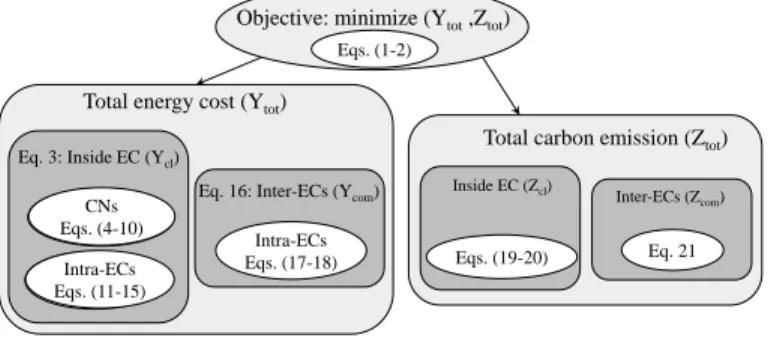
and 𝑍𝑡 𝑜𝑡 (see also Fig. 2 for an overview).
3.2.1 Overall cost formulation (𝑌𝑡 𝑜𝑡)
In order to determine 𝑌𝑡 𝑜𝑡, (3)-(16) formulate 𝑌𝑐𝑙 and (17)-(19)
formulate 𝑌𝑐 𝑜𝑚.
Costs incurred within the ECs: 𝑌𝑐𝑙 is the cost of incremental
energy of selected ECs (including both the CNs and the intra-cloud network) to place the newly requested components:
𝑌𝑐𝑙= Õ 𝑑∈𝐷 𝑃𝑈 𝐸𝑑· (𝑌0 𝑑+ 𝑌 00 𝑑) · 𝑦𝑑· 𝑆𝑑. (3)
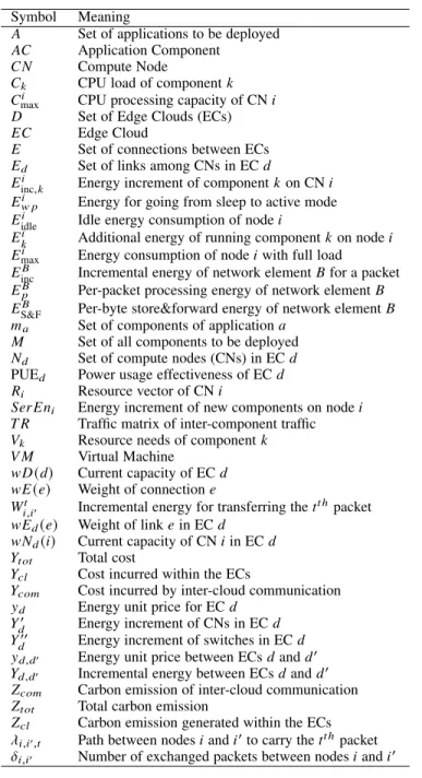
TABLE 2 Notation overview
Symbol Meaning
𝐴 Set of applications to be deployed 𝐴𝐶 Application Component
𝐶 𝑁 Compute Node
𝐶𝑘 CPU load of component 𝑘
𝐶max𝑖 CPU processing capacity of CN 𝑖 𝐷 Set of Edge Clouds (ECs) 𝐸 𝐶 Edge Cloud
𝐸 Set of connections between ECs 𝐸𝑑 Set of links among CNs in EC 𝑑
𝐸𝑖
inc,𝑘 Energy increment of component 𝑘 on CN 𝑖
𝐸𝑖
𝑤 𝑝 Energy for going from sleep to active mode
𝐸𝑖
idle Idle energy consumption of node 𝑖
𝐸𝑖
𝑘 Additional energy of running component 𝑘 on node 𝑖
𝐸𝑖
max Energy consumption of node 𝑖 with full load
𝐸𝐵
inc Incremental energy of network element 𝐵 for a packet
𝐸𝐵
𝑝 Per-packet processing energy of network element 𝐵
𝐸𝐵
S&F Per-byte store&forward energy of network element 𝐵
𝑚𝑎 Set of components of application 𝑎
𝑀 Set of all components to be deployed 𝑁𝑑 Set of compute nodes (CNs) in EC 𝑑
PUE𝑑 Power usage effectiveness of EC 𝑑
𝑅𝑖 Resource vector of CN 𝑖
𝑆 𝑒𝑟 𝐸 𝑛𝑖 Energy increment of new components on node 𝑖
𝑇 𝑅 Traffic matrix of inter-component traffic 𝑉𝑘 Resource needs of component 𝑘
𝑉 𝑀 Virtual Machine 𝑤 𝐷(𝑑) Current capacity of EC 𝑑 𝑤 𝐸(𝑒) Weight of connection 𝑒 𝑊𝑡
𝑖 ,𝑖0 Incremental energy for transferring the 𝑡 𝑡 ℎ
packet 𝑤 𝐸𝑑(𝑒) Weight of link 𝑒 in EC 𝑑
𝑤 𝑁𝑑(𝑖) Current capacity of CN 𝑖 in EC 𝑑
𝑌𝑡 𝑜𝑡 Total cost
𝑌𝑐𝑙 Cost incurred within the ECs
𝑌𝑐 𝑜𝑚 Cost incurred by inter-cloud communication
𝑦𝑑 Energy unit price for EC 𝑑
𝑌0
𝑑 Energy increment of CNs in EC 𝑑
𝑌00
𝑑 Energy increment of switches in EC 𝑑
𝑦𝑑 , 𝑑0 Energy unit price between ECs 𝑑 and 𝑑 0
𝑌𝑑 , 𝑑0 Incremental energy between ECs 𝑑 and 𝑑 0
𝑍𝑐 𝑜𝑚 Carbon emission of inter-cloud communication
𝑍𝑡 𝑜𝑡 Total carbon emission
𝑍𝑐𝑙 Carbon emission generated within the ECs
𝜆𝑖 ,𝑖0, 𝑡 Path between nodes 𝑖 and 𝑖 0
to carry the 𝑡𝑡 ℎ
packet 𝛿𝑖 ,𝑖0 Number of exchanged packets between nodes 𝑖 and 𝑖
0
Here, 𝑌𝑑0and 𝑌
00
𝑑 are the incremental energy consumption of CNs
and switches, respectively, caused by deploying new components
in EC 𝑑. PUE𝑑is the power usage effectiveness value and 𝑦𝑑is the
energy unit price for EC 𝑑. 𝑆𝑑is 1 if EC 𝑑 is selected, otherwise
0.
Equations (4)–(7) formulate 𝑌0
𝑑 and (12)–(16) formulate 𝑌
00 𝑑. For the sake of notational simplicity, we skip the index of ECs in these equations. 𝑌0 𝑑= Õ 𝑖∈ 𝑁𝑑 𝑆 𝑒𝑟 𝐸 𝑛𝑖· 𝑆𝑖. (4) 𝑆 𝑒𝑟 𝐸 𝑛𝑖= Õ 𝑘∈𝑀 𝐸𝑖 𝑖 𝑛𝑐 , 𝑘· 𝐿𝑘 ,𝑖. (5) 𝐸𝑖 𝑖 𝑛𝑐 , 𝑞= (𝐸 𝑖 𝑤 𝑝+ 𝐸 𝑖 𝑖 𝑑𝑙 𝑒) · 𝑆 𝑖 𝑆𝑙 𝑝+ 𝐸 𝑖 𝑘. (6) 𝐸𝑖 𝑘 = (𝐸 𝑖 𝑚𝑎 𝑥− 𝐸 𝑖 𝑖 𝑑𝑙 𝑒) · 𝐶𝑘 𝐶𝑖𝑚𝑎 𝑥 . (7)
Subject to the following constraints:
𝐿𝑘 ,𝑖≤ 𝑆𝑖. ∀𝑖 ∈ 𝑁𝑑, 𝑘∈ 𝑀, (8) Õ 𝑖∈ 𝑁𝑑 𝐿𝑘 ,𝑖=1. ∀𝑘 ∈ 𝑀, (9) Õ 𝑘∈𝑀 𝑉𝑘· 𝐿𝑘 ,𝑖≤ 𝑤𝑁𝑖. ∀𝑖 ∈ 𝑁𝑑. (10)
In (4), 𝑆𝑒𝑟 𝐸𝑛𝑖 is the incremental energy of running new
components on CN 𝑖. 𝑆𝑖 is 1 if at least one new component is
deployed to CN 𝑖, otherwise 0. In (5), 𝐸𝑖
𝑖 𝑛𝑐 , 𝑘 is the incremental
energy of running component 𝑘 on CN 𝑖. 𝐿𝑘 ,𝑖is 1 if component 𝑘
is allocated on CN 𝑖.
Equation (6) formulates 𝐸𝑖
𝑖 𝑛𝑐 , 𝑘 from (5), and where 𝐸 𝑖 𝑤 𝑝 is the energy needed by CN 𝑖 to go from sleep to active mode and 𝐸𝑖
Objective: minimize (Ytot,Ztot)
Total energy cost (Ytot)
Eq. 3: Inside EC (Ycl)
CNs Eqs. (4-10)
Intra-ECs Eqs. (11-15)
Eq. 16: Inter-ECs (Ycom)
Total carbon emission (Ztot)
Intra-ECs Eqs. (17-18) Inside EC (Zcl) Eqs. (19-20) Inter-ECs (Zcom) Eq. 21 Eqs. (1-2) CNs Eqs. (4-10) Intra-ECs Eqs. (11-15)
Fig. 2. Problem formulation diagram for the application allocation part
zero load). 𝑆𝑖
𝑆𝑙 𝑝 is 1 if CN 𝑖 is in sleep mode (0 if in active
mode) and 𝐸𝑖
𝑘 is the additional energy consumption of running
component 𝑘 on CN 𝑖. If CN 𝑖 is in sleep mode and receives the
first component, it needs to spend energy 𝐸𝑖
𝑤 𝑝to go from sleep to
active mode. If active but idle, CN 𝑖 consumes constant energy of 𝐸𝑖
𝑖 𝑑𝑙 𝑒; component 𝑘 adds 𝐸 𝑖
𝑘 to it. As the first component lets the
CN wake from sleep mode, the resulting energy consumption is 𝐸𝑖
𝑤 𝑝+ 𝐸 𝑖
𝑖 𝑑𝑙 𝑒+ 𝐸 𝑖
𝑘. But for components added to an already active
CN, the increase in energy is only 𝐸𝑖
𝑘. To compute 𝐸
𝑖
𝑘, we use the
following formula derived from [31] and [39]:
𝐸𝑖= 𝐸𝑖 𝑖 𝑑𝑙 𝑒+ | 𝑀 | Õ 𝑞=1 (𝐸𝑖 𝑞· 𝐿𝑞 ,𝑖) (11) In (7), 𝐸𝑖
𝑚𝑎 𝑥 is the energy consumption of CN 𝑖 with full
load, 𝐶𝑘 is the CPU load of component 𝑘 and 𝐶
𝑖
𝑚𝑎 𝑥 is the CPU
processing capacity of CN 𝑖.
The constraint, mentioned in (8), ensures that a component can be assigned only to a selected CN. Equation (9) guarantees that each component is assigned to exactly one CN and (10) guarantees that the total load of the components assigned to a CN does
not exceed its capacity. Recall that 𝑉𝑘 is the vector of requested
resources of component 𝑘 and 𝑤𝑁𝑖 is the current capacity of CN
𝑖.
After formulating 𝑌0
𝑑(incremental energy consumption of CNs
in EC 𝑑), (12)–(16) formulate 𝑌𝑑00 (incremental network energy
consumption in EC 𝑑). 𝑌𝑑00 is computed based on incremental
network energy stemming from the additional traffic between each pair of CNs in EC 𝑑 for running the new applications:
𝑌00 𝑑 = Õ 𝑖∈ 𝑁𝑑 Õ 𝑖0∈ 𝑁𝑑, 𝑖≠𝑖0 𝛿𝑖 ,𝑖0 Õ 𝑡=1 𝑊𝑡 𝑖 ,𝑖0. (12)
Here, 𝛿𝑖 ,𝑖0 is the number of exchanged packets between CNs 𝑖
and 𝑖0, and 𝑊𝑡
𝑖 ,𝑖0 is the incremental energy of network elements
between CNs 𝑖 and 𝑖0 for transferring the 𝑡𝑡 ℎ
packet. Note that in (12), only the selected CNs will be considered automatically,
because when there is no traffic between CNs 𝑖 and 𝑖0, then 𝛿
𝑖 ,𝑖0=
0. 𝛿𝑖 ,𝑖0is computed based on the characteristics of the components
allocated on CNs 𝑖 and 𝑖0and on the traffic matrix:
𝛿𝑖 ,𝑖0= Õ 𝑘∈𝑀 Õ 𝑘0∈𝑀 𝐿𝑘 ,𝑖· 𝐿𝑘0,𝑖0· 𝑡𝑟𝑘 , 𝑘0. (13)
𝐿𝑘 ,𝑖is 1 if component 𝑘 is allocated on CN 𝑖 (otherwise=0) and
𝑡𝑟𝑘 , 𝑘0 is the number of packets between components 𝑘 and 𝑘0.
𝑊𝑡 𝑖 ,𝑖0is computed as follows: 𝑊𝑡 𝑖 ,𝑖0= Õ 𝐵∈𝜆𝑖 ,𝑖0 , 𝑡 𝐸𝐵 inc. (14)
Here, 𝜆𝑖 ,𝑖0, 𝑡denotes the path between CNs 𝑖 and 𝑖
0to which the 𝑡𝑡 ℎ
packet is assigned. 𝐸𝐵
incis the incremental energy consumption of
network element 𝐵 for servicing a packet. The incremental energy consumption of network element 𝐵 is computed analogously to that of CNs (see (6)): 𝐸𝐵 inc= (𝐸 𝐵 wp+ 𝐸 𝐵 idle) · 𝑁 𝐵 Slp+ 𝐸 𝐵 . (15) In (15), 𝐸𝐵 is computed as indicated in [37]. 𝐸𝐵= 𝐸𝐵 𝑝+ 𝐸 𝐵 S& F𝐿 , (16) where 𝐸𝐵
𝑝 (i.e., per-packet processing energy) and 𝐸
𝐵
S&F(i.e., per-byte store-and-forward energy) are constants for a given switch or router configuration, and 𝐿 is the packet length.
Costs incurred by inter-cloud communication: 𝑌com is the
in-cremental energy of the network to transfer data between different ECs while running the newly requested applications.
𝑌com=
Õ
𝑑 , 𝑑0∈𝐷
𝑌𝑑 , 𝑑0· 𝑦𝑑 , 𝑑0· 𝑆𝑑· 𝑆𝑑0. (17)
where 𝑦𝑑 , 𝑑0 is the energy unit price for communication between
ECs 𝑑 and 𝑑0. 𝑌𝑑 , 𝑑0is the incremental energy between ECs 𝑑 and
𝑑0and is formulated in (18). 𝑌𝑑 , 𝑑0= 𝛿0 𝑑 , 𝑑0 Õ 𝑡=1 Õ 𝐵∈𝜆0 𝑑 , 𝑑0 𝐸𝐵 inc,𝑡. (18) 𝛿0
𝑑 , 𝑑0 is the number of exchanged packets and 𝜆 0
𝑑 , 𝑑0 is the set of
network elements between ECs 𝑑 and 𝑑0.
𝛿0 𝑑 , 𝑑0= Õ 𝑖∈𝑑 Õ 𝑖0∈𝑑0 Õ 𝑘∈𝑀 Õ 𝑘0∈𝑀 𝐿𝑘 ,𝑖· 𝐿𝑘0,𝑖0· 𝑡𝑟𝑘 , 𝑘0. (19)
where 𝐿𝑞 ,𝑖 is 1 if AC𝑞 is allocated on CN𝑖 of 𝐸𝐶𝑗 (otherwise=0)
and 𝐿𝑤 ,𝑖0is 1 if AC𝑤is allocated on CN𝑖0of 𝐸𝐶𝑗0(otherwise=0).
𝑡𝑟𝑞 , 𝑤 is the number of packets between AC𝑞 and AC𝑤.
3.2.2 Carbon emission formulation (𝑍𝑡 𝑜𝑡)
Recall that 𝑍𝑡 𝑜𝑡 is the sum of 𝑍𝑐𝑙 and 𝑍𝑐 𝑜𝑚, which are computed
as follows.
Intra-EC carbon emission: 𝑍𝑐𝑙 is the carbon emission caused
networks) to run the requests, computed as: 𝑍𝑐𝑙= Õ 𝑑∈𝐷 𝑃𝑈 𝐸𝑑· (𝑌0 𝑑+ 𝑌 00 𝑑) · 𝐶 𝐸𝑑· 𝑆𝑑. (20)
Recall that 𝑌𝑑0 and 𝑌
00
𝑑 (formulated in (4) and (12)) are the
incremental server (CN) energy and network energy, respectively,
in a selected EC 𝑑. 𝑆𝑑 is 1 if EC 𝑑 is selected, and 0 otherwise.
𝐶 𝐸𝑑 is the average carbon emission rate (in g/kW) of the energy
sources of EC 𝑑. It is computed as follows [4]:
𝐶 𝐸𝑑= Íℓ 𝑘=1𝐶 𝐸 𝑘 𝑑· 𝑟 𝑘 Íℓ 𝑘=1𝐶 𝐸 𝑘 𝑑 . (21) where 𝐶𝐸𝑘 𝑑 and 𝑟 𝑘
denote the electricity generated by energy source 𝑘 and its carbon emission rate, respectively.
Inter-EC carbon emission: 𝑍𝑐 𝑜𝑚 is the amount of incremental
carbon emission resulting from data transfer between the selected ECs:
𝑍𝑐 𝑜𝑚=
Õ
𝑑 , 𝑑0∈𝐷
𝑌𝑑 , 𝑑0· 𝐶𝐶 𝐸𝑑 , 𝑑0· 𝑆𝑑· 𝑆𝑑0. (22)
where 𝐶𝐶𝐸𝑑 , 𝑑0is the average carbon emission rate for
communi-cation between EC 𝑑 and 𝑑0. 𝑆𝑑is 1 if EC 𝑑 is selected (otherwise
0). 𝑌𝑑 , 𝑑0was defined in (18).
3.3 AC consolidation (migration) problem
Given a set 𝑀0 of ACs running on CNs of EC 𝑑, our goal is
to reduce the total energy consumption of running those ACs in 𝑑 using migrations. That is, given a number of ACs (already allocated on CNs) with their sizes and traffic matrix as an input, we aim to find a new feasible placement for ACs allocated on under-utilized CNs, minimizing: (1) the energy spent to run the ACs (by consolidating ACs to reduce the number of active CNs), (2) the total network overhead (by improving placement of ACs to reduce inter-AC traffic and the number of active switches), and (3) the overhead of AC migrations (by selecting a closer destination for migration in order to reduce network energy/traffic and using already activated switches to have minimum number of active switches).
AC consolidation should obtain maximum energy saving using appropriate AC migrations while consuming minimum possible energy for the migrations. The AC consolidation problem can be formulated as follows: maximize (𝜗 − 𝜗0− 𝜗00), 𝜗= 𝜗𝑠+ 𝜗𝑛, and 𝜗0= 𝜗0 𝑠+ 𝜗 0 𝑛 (23)
where 𝜗 and 𝜗0 denote the energy consumption in EC 𝑑 for
running the ACs before and after AC consolidation, respectively.
𝜗00is the amount of energy consumed by the migrations.
𝜗is composed of the energy consumption of running the ACs
on CNs (𝜗𝑠) and the energy consumption of the communication
among them (𝜗𝑛). 𝜗𝑠is computed as follows:
𝜗𝑠= Õ 𝑖∈ 𝑁𝑑 𝑆𝑖· Õ 𝑞∈𝑀0 𝐸𝑖 𝑞. (24)
Here, 𝑆𝑖 is 1 if at least one AC is allocated on CN 𝑖, and 𝐸
𝑖 𝑞 is
the energy consumption of running AC 𝑞 on CN 𝑖. 𝜗𝑠is computed
analogously to 𝑌𝑑0 (see (4)–(7)). The main difference is that 𝜗𝑠
contains the energy consumption of all allocated ACs on EC 𝑑,
while 𝑌𝑑0 considers only the energy consumption needed for the
new requests.
𝜗𝑛is the network energy consumption for the communication
among the already allocated ACs:
𝜗𝑛= Õ 𝑖∈ 𝑁𝑑 Õ 𝑖0∈ 𝑁𝑑 𝑖≠𝑖0 𝛿 𝑖 ,𝑖0 Õ 𝑡=1 𝐻 𝑖 ,𝑖0 Õ 𝜙=1 𝛼𝑡 𝑖 ,𝑖0, 𝜙· Õ 𝐵∈𝜆𝑖 ,𝑖0 , 𝜙 𝐸𝐵 𝑖 𝑛𝑐. (25)
H𝑖 ,𝑖0 is the number of available paths between CN 𝑖 and CN 𝑖
0. 𝛼𝑡
𝑖 ,𝑖0, 𝜙is 1 if the 𝜙 𝑡 ℎ
path is selected. 𝜗𝑛is computed analogously
to 𝑌𝑑00 (see (12)–(16)). The main difference is that 𝜗𝑛 includes
the communication energy consumption of all already allocated
ACs on EC 𝑑, while 𝑌𝑑00considers only the communication energy
consumption for the new requests.
𝜗0 is calculated in the same way as 𝜗, but using the new
allocation after the migrations have been effectuated.
𝜗00is the energy needed for the migration of the ACs selected
by the AC consolidation algorithm. 𝜗00= Õ 𝑞∈𝑀0 𝑆𝑞· 𝜗 00 𝑞 ,(𝑖,𝑖0). (26)
where 𝑆𝑞 is 1 if 𝐴𝐶𝑞 is migrated, otherwise 0. 𝜗
00
𝑞 ,(𝑖,𝑖0) is the
energy needed to migrate 𝐴𝐶𝑞from its source CN 𝑖 to destination
CN 𝑖0: 𝜗00 𝑞 ,(𝑖,𝑖0) = 𝑇𝑞 Õ 𝑡=1 𝐻𝑖 ,𝑖0 Õ 𝜙=1 𝛽𝑡 𝑖 ,𝑖0, 𝜙· Õ 𝐵∈𝜆𝑖 ,𝑖0 , 𝜙 𝐸𝐵 𝑖 𝑛𝑐. (27)
𝑇𝑞 is the number of needed packets to transfer AC𝑞. 𝑇𝑞 is
computed based on the size of AC𝑞 and packet size 𝐿 (i.e.,
𝐴𝐶𝑞
𝐿 ).
H𝑖 ,𝑖0is the number of available paths between CN 𝑖 and destination
CN 𝑖0. 𝛽𝑖 ,𝑖0, 𝜙is 1 if the 𝜙 𝑡 ℎ
path is selected.
4
D
YNAMIC ENERGY COST AND CARBONEMISSION
-
EFFICIENT APPLICATION PLACEMENTMETHOD
(DECA)
To describe DECA, first we introduce its general three-phase mechanism. Then, we present the DECA logical architecture and describe in detail each of its components.
4.1 General mechanism
DECA consists of three main phases: (1) Pre-allocation, (2) Allocation, and (3) Placement improvement.
Phase 1—Pre-allocation. Based on the requested application components, the components’ traffic matrix, the available ECs and CNs, this phase tentatively determines the best resources considering cost and carbon emission. This is done in two steps (see Algorithm 1). Step 1 pre-selects ECs and pre-distributes the components to them simultaneously (joint EC selection and component distribution). Step 2 chooses CNs in each pre-selected EC and pre-allocates components on them simultaneously (joint CN selection and component placement). In both steps, we first create candidate subgraphs and then select the best subgraph in terms of overall energy cost and carbon emission.
If a component is distributed to EC 𝑑 in Step 1, then it is tried to be allocated on a compute node within EC 𝑑 in Step 2. This will be normally successful since the decisions in Step 1 ensure that the total capacity of an EC is sufficient for the total demand of components mapped to that EC. However, this is only a necessary but not sufficient condition for being able to place the set of ACs
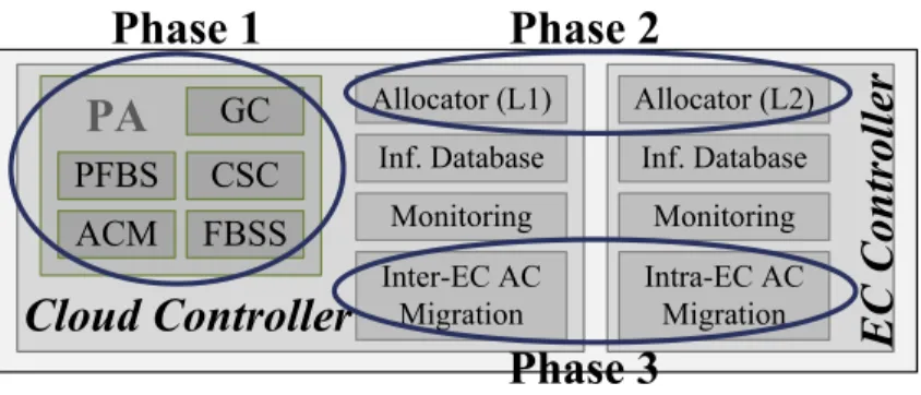
Fig. 3. Logical architecture of DECA
in this EC. It may turn out in Step 2 that an AC cannot be allocated in the intended EC. In this case, the AC and its related ACs are re-allocated to another EC.
Based on the pre-allocation observation, this phase finds the best resources for the requested ACs and offers them for allocation in Phase 2.
Phase 2—Allocation. Phase 2 actually allocates the requested ACs on the resources finally selected in Phase 1.
Phase 3—Placement improvement. Phase 3 is in charge of man-aging already allocated ACs. It has two main objectives: (1) energy saving: it includes inter-EC and intra-EC AC migration methods and continually minimizes energy consumption of each EC to optimize energy cost and carbon emission, (2) SLA violation prevention: by migrating ACs from overloaded CNs, it prevents SLA violation.
4.2 DECA architecture
As mentioned in Section 3.1, we assume a cloud controller and EC controllers in a hierarchical distributed EC architecture. Note that the cloud controller is a logical component which might be implemented in a physically distributed way enabling both load balancing and fault tolerance, but this is beyond the scope of the paper. In each time slot, the cloud controller selects appropriate resources (ECs, CNs and paths) for the received AC requests and distributes the ACs to the chosen ECs. Inside each EC, the EC controller places the received AC requests on the chosen CNs. Moreover, in each time period 𝑇 , the cloud controller runs inter-EC AC migration and, right after that, each inter-EC controller uses intra-EC AC migrations to continually optimize cost and carbon emission of the EC and also to prevent SLA violations (CN overloading).
To offer a better view about the DECA mechanism, we mapped the three phases of DECA on its logical architecture (see Fig. 3). Cloud and EC controller include some modules which are described next.
4.2.1 Cloud controller modules
Pre-Allocator (PA). This module (see Algorithm 1) reads gen-eral cloud information from the Information database, creates a complete graph of ECs and complete graph of CNs inside each EC, calls the appropriate sub-modules to pre-allocate the ACs, and finally sends the determined placement information to the Allocator (Level 1 and 2) modules. The PA module includes several sub-modules that we will describe as follows:
Algorithm 1: Pre-Allocator(𝐺0,{𝐺𝑖}, 𝑇 , 𝑇 𝑅) → (c, f,
e[f])
1 (a, b) = CSC(𝐺0, M, TR); /*a: subgraphs of ECs, b:
ACs on them*/
2 c = FBSS (a,b); /*c: the best subgraph of ECs */
3 foreach 𝐸𝐶 ∈ c do
4 (d, e) = CSC(𝐺𝐸 𝐶 , b[c][EC] , TR);
5 /*d: subgraph of CNs, e: ACs on them*/
6 f = FBSS(d, e); /*f: the best subgraph of CNs for
EC*/
7 /*c: selected ECs, f: selected CNs inside ECs, e: way of
placing ACs on CNs*/
Graph Creator (GC). The GC module creates a complete graph of ECs and complete graph of CNs inside each EC based on general cloud information in the Information database.
AC Mapper (ACM). The ACM module (see Algorithm 2) re-ceives a candidate vertex 𝑣 (which may represent an EC or a CN) with its current capacity and a set 𝑋 of ACs with their traffic matrix
𝑇 𝑅as input. Starting from each AC 𝑞 ∈ 𝑋, ACM determines a
subset 𝑌𝑞 of 𝑋 that fits on 𝑣. 𝑌𝑞 is grown greedily: in each step,
the AC from 𝑋 \ 𝑌𝑞 is chosen that has the largest traffic with
the ACs already in 𝑌𝑞, and is added to 𝑌𝑞 if 𝑣 still has sufficient
capacity. After creating a subset starting from each AC 𝑞, ACM selects the subset with highest inter-AC traffic and maps it to 𝑣.
Algorithm 2: ACM(𝑣, X, TR) → highest traffic 𝑌𝑖
1 foreach 𝐴𝐶𝑞∈ 𝑋 do
2 𝑌𝑖 = {};
3 if 𝑣 has enough capacity for AC𝑞then
4 Add AC𝑞to 𝑌𝑖;
5 while 𝑣 has enough capacity for 𝑌𝑖 and 𝑌𝑖≠ 𝑋do
6 Let 𝑉 ∈ 𝑋 \ 𝑌𝑖 have the highest total traffic
with ACs in 𝑌𝑖;
7 if 𝑣 has enough capacity for 𝑌𝑖∪ {𝑉 } then
8 Add 𝑉 to 𝑌𝑖;
9 /* return the 𝑌𝑖with highest inter-AC traffic */
Candidate Subgraph Creator (CSC). As Algorithm 3 shows, this module receives a weighted graph 𝐺 = (𝑉 , 𝐸, 𝑤𝑉 , 𝑤𝐸), a list of ACs M[ ] and their traffic information TR as input and returns
aim of CSC is to determine for each 𝑣𝑖 ∈ 𝑉 (1 ≤ 𝑖 ≤ |𝑉 |) an
induced subgraph 𝐺0(𝑣𝑖) with sufficient total capacity for hosting
the ACs and optimized overall cost and carbon emission. 𝐺0(𝑣𝑖)
is grown from {𝑣𝑖} as starting point by iteratively adding one
vertex a time. The already selected vertices of 𝐺0(𝑣𝑖) and their
allocated ACs are stored in arrays 𝑆 [𝑖] and 𝑆𝑣[𝑖] respectively. In
each step, CSC checks whether the selected vertices have sufficient
total capacity. If this is the case, 𝐺0(𝑣𝑖) is finished. Otherwise, the
PFBS module is called to select one more vertex for inclusion in
𝑆, and the cycle continues, until the total capacity of the selected
vertices is sufficient. Then, 𝐺0(𝑣𝑖) is the subgraph induced by
𝑆[𝑖], with its allocated ACs stored in 𝑆𝑣[𝑖]. This way, a subgraph
is created for each vertex 𝑣𝑖as a starting point yielding altogether
|𝑉 | candidate subgraphs.
Trying each vertex as a starting point is important because
the subgraph formed starting from 𝑣𝑖will often be biased towards
vertices in the proximity of 𝑣𝑖; taking the best one of the candidate
subgraphs helps to find a globally optimal one. In principle, it would also be possible to consider all subgraphs of 𝐺 with suf-ficient total capacity. However, the number of all such subgraphs can be exponential, making this approach intractable in practice. In contrast, our method is a faster, polynomial-time heuristic. Prediction and Fuzzy Sets-Based Selector (PFBS). Whenever
CSC needs to add a new vertex (i.e., 𝑣𝑘) to a candidate subgraph
𝐺0(𝑣𝑖) being generated, it calls the PFBS module (recall that the
subgraph 𝐺0(𝑣𝑖) formed starting from 𝑣𝑖). As Algorithm 4 shows,
PFBS receives a graph 𝐺, a list of already selected vertices in
subgraph 𝐺0(𝑣𝑖) (i.e., 𝑆 [𝑖]), a set of unallocated ACs (i.e., 𝑋), AC
traffic information (i.e., 𝑇 𝑅), and a variable 𝐻 as input. PFBS
returns the most cost/carbon effective vertex 𝑣𝑘 ∈ 𝑉 \ 𝑆 and
selected ACs on it (𝑆𝑣) to be included in 𝐺
0(𝑣
𝑖). H = 1 means
all vertices of 𝐺 will be used for allocating the requested ACs and so we do a simple random vertex selection to save time. 𝑉 \ 𝑆 are the vertices still available in 𝐺 for selection. Selecting the best vertex based on a single metric (e.g., only cost or carbon emission) is relatively easy. But selecting the best vertex according to two, sometimes conflicting, metrics simultaneously is more challenging. This is where Fuzzy Sets [7] are helpful to trade off the two metrics and thus select the best vertex. Another challenge is that, to be fast, we must make local decisions on the next vertex; but ignoring the effect of later decisions could lead to poor results. For this reason, we propose a combination of the Fuzzy
Sets technique and the 𝐴∗ algorithm [6] to get the benefits of
both appropriate decisions for multiple metrics (using fuzzy sets)
and global decisions (using 𝐴∗) together. An example showing the
benefits of using 𝐴∗is given in the Appendix.
Equations (28)–(38) detail our proposed method. PFBS uses a fuzzy set of all possible (EC or CN) candidates (i.e., 𝑉 \ 𝑆). There is a membership function 𝑐() for this set to map each candidate to
a membership value in the range [0, 1]. For a candidate 𝑣𝑘 ∈ 𝑉 \ 𝑆,
𝑐(𝑣𝑘) is computed based on its cost and carbon emission.
Inspired by the 𝐴∗ algorithm, 𝑐(𝑣
𝑘) is made up of two
functions: 𝑔(𝑣𝑘) is based on the immediate costs and carbon
emission incurred by selecting the candidate 𝑣𝑘, while ℎ(𝑣𝑘) is
based on an estimate of the costs and carbon emission that will
be incurred in the future if 𝑣𝑘 is selected now. This estimation
aspect of the 𝐴∗algorithm can give a global optimization view. It
also helps to consider the capacity of each candidate in addition to
cost and carbon emission. Hence, for a candidate 𝑣𝑘 ∈ 𝑉 \ 𝑆, the
Algorithm 3: CSC(G, M[ ], TR) → (S, S𝑣)
1 𝑆[ ] [ ] = { }, 𝑆𝑣[ ] [ ] [ ] = { }, copy members of array
M[ ] into a set𝑋;
2 𝑇𝑠: Total requested of|𝑋 |ACs, 𝑇𝑛: Total available
capacity of G
3 H = 1 if all nodes of G will be used for placing the
requested ACs; else H =|𝑉 |;
4 for i=1 to H do 5 𝑆[𝑖][0] =𝑣𝑖, j = 0, 𝑋 0= { }, 𝑆𝑣[𝑖][j][ ]← ACM(𝑣𝑖, 𝑋\ 𝑋 0, TR), 6 𝑋0=𝑋0∪ 𝑆𝑣[i] [ 𝑗 ],𝑇𝑐 = wv𝑖; /*𝑇𝑐:Total current capacity,*/ 7 while 𝑇𝑐< 𝑇𝑠do 8 j←j+1; 9 (𝑣𝑛𝑒 𝑤, 𝑆𝑣[𝑖 ] [ 𝑗 ]) =PFBS(𝐺, 𝑆 [𝑖 ], 𝑋 \ 𝑋 0, 𝑇 𝑅, H );
10 /*selects one more vertex and its ACs*/
11 𝑋0=𝑋0∪ 𝑆𝑣[i] [ 𝑗 ], S[i][j] =𝑣𝑛𝑒 𝑤;
12 𝑇𝑐=𝑇𝑐 + v𝑣𝑛𝑒 𝑤; /*v𝑣𝑛𝑒 𝑤is resource vector of
𝑣𝑛𝑒 𝑤*/
13 /*if not all ACs could be allocated*/
14 if 𝑋 ≠ 𝑋0then
15 𝑋00= { }; /*Set of ACs to move to another EC*/ 16 foreach 𝑥0∈ 𝑋0do
17 add x’ to𝑋00;
18 foreach 𝑥 ∈ 𝑋 do
19 if x’ has relation with x then
20 add x to𝑋00;
21 if x is already pre-allocated then
22 remove x from its CN and EC;
23 else
24 /*x is also a member of set X’*/
25 remove x from X’;
26 /*allocate𝑋00to an appropriate EC*/
27 (S’, S’𝑣) = CSC(G\S[i], X”, TR)
28 S = S∪S’, S𝑣 = S𝑣 ∪S’𝑣;
29 /*returns candidate subgraphs with allocated ACs*/
Algorithm 4: PFBS(G(V,E,wV,wE) → (selected,
𝑆𝑣[𝑣𝑘])
1 𝑐𝑚𝑎 𝑥= −1;
2 if 𝐻 == 1 then
3 select a𝑣𝑘 ∈ 𝑉 \ 𝑆randomly where
𝑣 𝑐 𝑝𝑢 𝑘 < 𝑆 𝐿 𝐴𝑇 ℎ𝑟 𝑒𝑠 ℎ 𝑜𝑙 𝑑; 4 𝑆𝑣[𝑣𝑖] [ 𝑗 ] ←ACM(w𝑣𝑖, X, TR); 5 return (𝑣𝑘,𝑆𝑣[𝑣𝑘]); 6 foreach 𝑣𝑘 ∈ 𝑉 \ 𝑆 do 7 if 𝑣𝑐 𝑝𝑢 𝑘 < 𝑆 𝐿 𝐴𝑇 ℎ𝑟 𝑒𝑠 ℎ 𝑜𝑙 𝑑 then 8 𝑆𝑣[𝑣𝑖] [ 𝑗 ] ←ACM(w𝑣𝑘, X, TR); 9 compute𝑐( 𝑣𝑘)using (28)–(38); 10 if 𝑐 ( 𝑣𝑘) > 𝑐𝑚𝑎 𝑥then 11 𝑐𝑚𝑎 𝑥= 𝑐 ( 𝑣𝑘), selected= 𝑣𝑘;
𝐴∗-based membership value is
The algorithm selects the candidate with the largest 𝑐(𝑣𝑘) value.
Here, 𝑔(𝑣𝑘) computes a membership value based on the increment
in overall cost and carbon emission (for both server and network
resources) incurred by selecting 𝑣𝑘:
𝑔(𝑣𝑘) = 1 − 𝐾1(𝑣𝑘) · 𝐾2(𝑣𝑘). (29)
where 𝐾1(𝑣𝑘) and 𝐾2(𝑣𝑘) are normalized values of cost and
carbon emission (in range of [0,1]) respectively. Equation (29)
ensures that maximizing 𝑔(𝑣𝑘) leads to low values for both cost
and carbon emission. Equations (30) and (31) normalize cost and carbon emission respectively.
𝐾1(𝑣𝑘) = 𝑆𝑣 𝑘· 𝑃𝑣𝑘 + 𝑁𝑣𝑘· 𝑃 0 𝑣𝑘 𝑆𝑚𝑎 𝑥· 𝑃𝑚𝑎 𝑥+ 𝑁𝑚𝑎 𝑥· 𝑃𝑚𝑎 𝑥0 . (30) 𝐾2(𝑣𝑘) = 𝑆𝑣 𝑘 · 𝐶 𝐸𝑣𝑘 + 𝑁𝑣𝑘· 𝐶 𝐸 0 𝑣𝑘 𝑆𝑚𝑎 𝑥· 𝐶 𝐸𝑚𝑎 𝑥+ 𝑁𝑚𝑎 𝑥· 𝐶 𝐸𝑚𝑎 𝑥0 . (31)
where S𝑣𝑘 is the incremental energy of 𝑣𝑘 caused by running the
new ACs and S𝑚𝑎 𝑥 is the incremental energy of the candidate
with the maximum incremental energy. P𝑣𝑘 and P
0
𝑣𝑘 (for network
elements inside 𝑣𝑖) are the energy price in the location of 𝑣𝑖.
However, for inter-EC network elements, we consider P0𝑣𝑘 as
average of the energy prices. P𝑚𝑎 𝑥 and P
0
𝑚𝑎 𝑥 are the maximum
energy price among all locations. CE𝑣𝑘 and CE
0
𝑣𝑘 (for network
elements inside 𝑣𝑘) are the carbon emission rate in location of 𝑣𝑘.
For inter-EC network elements, CE0𝑣𝑘 is the average of the carbon
rates. CE𝑚𝑎 𝑥 and CE
0
𝑚𝑎 𝑥 are the maximum carbon rate among
all locations. N𝑣𝑘 is the incremental energy of network elements
caused by adding the candidate 𝑣𝑘 to the subgraph 𝐺
0(𝑣 𝑖): 𝑁𝑣 𝑘 = Õ 𝑣𝑗∈𝑆 [𝑖 ] 𝑛𝑣 𝑘, 𝑣𝑗 . (32)
where n𝑣𝑘, 𝑣𝑗 is the incremental energy of transferring data from
candidate 𝑣𝑘to the already selected 𝑣𝑗in 𝐺
0(𝑣
𝑖) (recall that 𝐺
0(𝑣 𝑖)
is the subgraph that is grown from 𝑣𝑖 and S[i] holds the current
vertices of 𝐺0(𝑣𝑖)). For EC selection, n𝑣𝑘, 𝑣𝑗is computed based on
(18) whereas for CN selection, (14) is used. PFBS calls for each
candidate 𝑣𝑘 the ACM module to detect allocated ACs on 𝑣𝑘and
then computes 𝛿𝑘 , 𝑗 for CNs based on (13) and for ECs based on
(19). Recall that (14) also selects the best path between two CNs.
ℎ(𝑣𝑘) computes a membership value based on an estimate of
the increment in overall cost and carbon emission caused by the vertices that we will have to select later on to accommodate all the
𝑀ACs. ℎ(𝑣𝑘) = 1 − 𝐾0 1(𝑣𝑘) · 𝐾 0 2(𝑣𝑘). (33) where 𝐾10(𝑣𝑘) and 𝐾 0
2(𝑣𝑘) are normalized values of the estimated
cost and carbon emission (in range of [0,1]) respectively.
𝐾0 1(𝑣𝑘)= 𝑦·𝑆𝑎·𝑃𝑎+𝑈·𝑁𝑎·𝑃 0 𝑎 𝑦·𝑆𝑚𝑎 𝑥·𝑃𝑚𝑎 𝑥+𝑈·𝑁𝑚𝑎 𝑥·𝑃 0 𝑚𝑎 𝑥 . (34) 𝐾0 2(𝑣𝑘)= 𝑦·𝑆𝑎·𝐶 𝐸𝑎+𝑈·𝑁𝑎·𝐶 𝐸 0 𝑎 𝑦·𝑆𝑚𝑎 𝑥·𝐶 𝐸𝑚𝑎 𝑥+𝑈·𝑁𝑚𝑎 𝑥·𝐶 𝐸 0 𝑚𝑎 𝑥 . (35)
where 𝑦 and 𝑈 are the estimated number of vertices and edges
(network paths) to be added later to the subgraph 𝐺0(𝑣𝑖), when
allocating the remaining ACs. S𝑎 is the estimated average and
S𝑚𝑎 𝑥the maximum possible incremental energy for a new vertex,
N𝑎 is the estimated average and N𝑚𝑎 𝑥 the maximum possible
incremental energy of the network for the further edges. P𝑎 and
P0𝑎are the average, P𝑚𝑎 𝑥and P
0
𝑚𝑎 𝑥 the maximum price of energy
for vertices and edges, respectively.
To estimate 𝑈, recall that 𝐺 is a complete graph, so that each
new node added to a subgraph 𝐺0(𝑣𝑖) with 𝑧 vertices will add 𝑧
new edges. After adding 𝑣𝑘to the subgraph 𝐺
0(𝑣
𝑖) with 𝑧 vertices,
it will consist of 𝑧 +1 vertices, so adding further vertices will lead
to 𝑧 +1, 𝑧 + 2, . . . new edges. Hence, if 𝑦 further vertices will have
to be selected after 𝑣𝑘, we have
𝑈= ( 𝑧+1)+( 𝑦−1) Õ 𝑘=𝑧+1 𝑘= 𝑧 · 𝑦 + 𝑦· (𝑦 + 1) 2 . (36)
The value of 𝑦 can be calculated as follows:
𝑦= | 𝑀 | − ( (Í 𝑣𝑗∈𝑆 [𝑖 ] 𝐹(𝑣𝑗)) + 𝐹 (𝑣𝑘)) 𝐴𝑣 . (37)
where | 𝑀 | is the total number of newly requested ACs, 𝐹 (𝑣𝑗) is
the number of allocated ACs on vertex 𝑣𝑗 of subgraph 𝐺
0(𝑣 𝑖), Í
𝑣𝑗∈𝑆 [𝑖 ]
𝐹(𝑣𝑗) is the number of allocated ACs till now on 𝐺0(𝑣𝑖),
𝐹(𝑣𝑘) is the number of ACs that can be allocated if 𝑣𝑘 is chosen
next, and 𝐴𝑣 is the average capacity of all vertices.
It remains to estimate N𝑎, the average network energy
con-sumption for the edges that will be added to the subgraph 𝐺0(𝑣𝑖)
in subsequent steps. One possibility is to use the average network energy consumption among all CNs. This would be a good estimate if we sampled edges randomly. However, our algorithm is biased towards edges of lower energy, so that the overall average may be an overestimate. A better estimate is the average energy consumption of the edges that the algorithm has selected
so far, i.e., the edges within the subgraph 𝐺0(𝑣𝑖) extended with
𝑣𝑘 (denoted as Al). However, when selecting the second vertex,
𝐺0(𝑣𝑖) has only one vertex and no edge, so in this case, we use
the average network energy consumption between the first vertex
(i.e., 𝑣𝑖) and all other vertices:
𝑁𝑎= Í 𝑣𝑗 ∈𝐴𝑙 Í 𝑣ℓ ∈𝐴𝑙\{𝑣𝑗 } 𝑛( 𝑣𝑗𝑣ℓ) ( 𝑧+1) 𝑧/2 if 𝑧 >1 Í 𝑣 𝑗 ∈𝑉\ 𝐴𝑙 𝑛( 𝑣𝑖, 𝑣𝑗) 𝑁−1 if 𝐴𝑙 = {𝑣𝑖} (38)
Putting all the pieces together, we get a fairly good estimate of
the overall energy cost and carbon emission when selecting 𝑣𝑖.
Based on these estimates, the algorithm can select the best 𝑣𝑖(see
Algorithm 4).
Fuzzy Sets-based Best Subgraph Selector (FBSS). This module receives as input a set of subgraphs (i.e., S) along with a list of
allocated ACs on their vertices (i.e., S𝑣). FBSS selects the most
appropriate subgraph in terms of cost and carbon emission. While selecting the best subgraph based on only cost or carbon emission is easy, the simultaneous optimization of the two metrics is more challenging. We use fuzzy sets to solve this.
As Algorithm 5 shows, FBSS computes for each 𝐺0(𝑣𝑖) the
overall cost (𝐶𝑜𝑠𝑡𝑖) and carbon emission (𝐶𝑎𝑟𝑖) using (39)–(40).
Recall that vertices of a subgraph 𝐺0(𝑣
𝑖) stored in S[i] and also
S𝑣[i] consists of the allocated ACs of 𝐺
0(𝑣 𝑖). 𝐶 𝑜 𝑠𝑡𝑖= Õ 𝑣∈𝑆 [𝑖 ] Õ 𝑗∈𝑆𝑣[𝑖 ] [𝑣 ] 𝐸𝑣 𝑖 𝑛𝑐 , 𝑗· 𝑦𝑣+ Õ 𝑣 , 𝑣0∈𝑆 [𝑖 ] 𝑌𝑣 , 𝑣0· 𝑦𝑣 , 𝑣0. (39) 𝐶 𝑎𝑟𝑖= Õ 𝑣∈𝑆 [𝑖 ] Õ 𝑗∈𝑆𝑣[𝑖 ] [𝑣 ] 𝐸𝑣 𝑖 𝑛𝑐 , 𝑗·𝐶 𝐸𝑣+ Õ 𝑣 , 𝑣0∈𝑆 [𝑖 ] 𝑌𝑣 , 𝑣0·𝐶 𝐸𝑣 , 𝑣0. (40) where 𝐸𝑣
𝑖 𝑛𝑐 , 𝑗 (incremental energy of vertex v of 𝐺 0(𝑣
𝑖) caused by
Algorithm 5: FBSS(S[ ][ ],𝑆𝑣[ ][ ][ ]) → (selected)
1 𝐹𝑚𝑎 𝑥= −1, i=0;
2 while 𝑆 [𝑖 ] ≠ 𝑛𝑢𝑙𝑙 do
3 compute cost of S[i] using (39);
4 compute carbon emission of S[i] using (40);
5 compute𝐹𝑖using (41);
6 if 𝐹𝑖 > 𝐹𝑚𝑎 𝑥then
7 F𝑚𝑎 𝑥=𝐹𝑖, selected = S[i];
8 i = i+1;
9 /* returns the best subgraph */
network energy between vertices v and v0) for EC subgraphs is
computed from (18) and for CN subgraphs from (12)–(16). 𝑦𝑣
and 𝑦𝑣 , 𝑣0(for network elements inside an EC) are the energy price
in location of the EC. For inter-EC network elements, we consider 𝑦𝑣 , 𝑣0as average of the energy prices. CE𝑣and CE
0
𝑣 , 𝑣0(for network elements inside an EC) are the carbon emission rate in location of
that EC. For inter-EC network elements, CE0𝑣 , 𝑣0is the average of
the carbon emission rates. As we have the list of allocated ACs for each vertex, the number of exchanged packets between two nodes is easily computed for CNs from (13) and for ECs from (19).
FBSS then computes membership value of S[i] using the membership function shown in (41).
𝐹𝑖=1 − 𝐶 𝑜 𝑠𝑡𝑖 𝐶 𝑜 𝑠𝑡𝑚𝑎 𝑥 · 𝐶 𝑎𝑟𝑖 𝐶 𝑎𝑟𝑚𝑎 𝑥 . (41)
where 𝐶𝑜𝑠𝑡𝑚𝑎 𝑥 and 𝐶𝑎𝑟𝑚𝑎 𝑥 are the maximum possible cost
and carbon emission for running the new requests, respectively. Finally, the subgraph with highest membership value is selected. Allocator (Level 1). Based on AC allocation information from the Pre-Allocator module, this module sends each AC request to the chosen EC controller.
Monitoring. Cooperating with EC controllers, this module con-tinuously monitors the cloud environment and updates the Cloud Information Database.
Information Database. All information related to the distributed EC is stored in this module.
Inter-EC AC Migration. The energy price and carbon emission rate not only can be different from EC to EC (i.e., in different locations) but can also vary with time (e.g., even on an hour-to-hour basis). Therefore, the overall energy cost or carbon emission may be reduced by shifting portions of the ACs to ECs that currently offer better energy prices and/or carbon emission rates [25]. Because of the similar decision-making for inter-EC and intra-EC AC migration, we describe them together in Section 4.2.2.
4.2.2 EC controller modules
The EC controller receives AC requests along with target CNs from the cloud controller. The EC controller allocates the ACs on the selected CNs (Allocator level 2), monitors the CNs (EC Monitoring) and gathers information of the EC and sends it to the cloud controller. To keep optimizing cost and carbon emission while preventing SLA violations, a Migration module is also used. Allocator (Level 2). This module executes the AC allocation, as determined by the cloud controller.
Monitoring. Cooperating with CN controllers, this module con-tinuously monitors the EC and updates the Information Database.
Algorithm 6: AC Migration-Under-utilized CNs (S,D) 1 𝑅𝑜𝑢 𝑛𝑑𝑚𝑖 𝑛= ∞, m=1, copy sets S to S 0and D to D0 2 while m != |𝑆0| do 3 for i=1 to |𝑆 | do 4 𝑇𝑠𝑡 𝑎 𝑦=0,𝑇𝑚𝑔𝑟=0 5 foreach AC𝑞on CN𝑖 ∈ S do 6 F𝑚𝑖 𝑛= ∞ 7 foreach CN𝑖0∈ D do 8 compute F( 𝐴𝐶𝑞,𝐶 𝑁𝑖0) (see (42)) 9 if F( 𝐴𝐶𝑞,𝐶 𝑁𝑖0) <F𝑚𝑖 𝑛then 10 F𝑚𝑖 𝑛= F( 𝐴𝐶𝑞,𝐶 𝑁𝑖0), Index[i][q]= 𝐶 𝑁𝑖0
11 if Index[i][q] is full, remove it from Set D
12 compute F( 𝐴𝐶𝑞,𝐶 𝑁𝑖)(see (42))
13 𝑇𝑠𝑡 𝑎 𝑦=𝑇𝑠𝑡 𝑎 𝑦+F( 𝐴𝐶𝑞,𝐶 𝑁𝑖),𝑇𝑚𝑔𝑟=𝑇𝑚𝑔𝑟+F𝑚𝑖 𝑛
14 if (𝑇𝑠𝑡 𝑎 𝑦+ 𝐸𝑖 𝑑𝑙 𝑒> 𝑇𝑚𝑔𝑟)then
15 pre-migrate (map) each AC𝑞of𝐶 𝑁𝑖 to
Index[i][q], Round[i]=Round[i]+𝑇𝑚𝑔𝑟
16 else
17 Round[i] = Round[i]+𝑇𝑠𝑡 𝑎 𝑦+ 𝐸𝑖 𝑑𝑙 𝑒,
Index[i][q]=CN𝑖
18 do a circular shift for set S0
19 if (𝑅𝑜𝑢𝑛𝑑𝑚𝑖 𝑛> 𝑅𝑜𝑢 𝑛𝑑[𝑖 ]) then
20 𝑅𝑜𝑢 𝑛𝑑𝑚𝑖 𝑛=Round[i], copy array Index[][] to array
Temp[][]
21 copy sets S0to S and D0to D, m++
22 migrate based on array Temp information
Information Database. All information related to the EC is stored in this module.
Intra-EC AC Migration. The aim of this module is twofold: (i) to prevent SLA violations of over-utilized CNs, and (ii) to optimize energy consumption (and thus costs and carbon emission) by emptying and switching off under-utilized CNs.
Inspired by [20], we consider three thresholds: 𝑇𝐿 (low), 𝑇𝑀
(middle) and 𝑇𝐻 (high). These thresholds divide a CN’s possible
workload situations into four states: under-utilized (under 𝑇𝐿),
light (between 𝑇𝐿 and 𝑇𝑀), moderate (between 𝑇𝑀 and 𝑇𝐻), and
over-utilized (above 𝑇𝐻).
The goal of this workload classification is to easily find source and destination CNs for AC migration as follows: (1) all ACs on an under-utilized CN 𝑖 should be migrated to CNs with light workload; then, 𝑖 can be switched to sleep mode to save energy; (2) to prevent SLA violations, some ACs on over-utilized CNs must be migrated to other CNs (usually to CNs with light workloads); (3) ACs on lightly or moderately loaded CNs are not migrated to avoid unnecessary migration cost [20], [40].
For over-utilized CNs, migrating some ACs is mandatory to prevent SLA violation, even if this increases energy consumption. In contrast, migration of ACs from under-utilized CNs should be carried out only if it improves the energy balance, i.e., the energy consumption of the migrations is less than the energy reduction achieved.
Algorithm 6 shows the proposed AC migration mechanism for under-utilized CNs. In each time period, first, all under-utilized CNs are put in a set 𝑆 and potential migration destinations are collected in a set 𝐷. These are primarily the lightly-loaded CNs, but if there is no such CN, we select moderately-loaded CNs