An integration technique for 3D curved cracks and branched discontinuities within the eXtended Finite Element Method

HAL Id: hal-01455394

https://hal.archives-ouvertes.fr/hal-01455394

Submitted on 3 Feb 2017

HAL is a multi-disciplinary open access archive for the deposit and dissemination of sci-entific research documents, whether they are pub-lished or not. The documents may come from teaching and research institutions in France or abroad, or from public or private research centers.

L’archive ouverte pluridisciplinaire HAL, est destinée au dépôt et à la diffusion de documents scientifiques de niveau recherche, publiés ou non, émanant des établissements d’enseignement et de recherche français ou étrangers, des laboratoires publics ou privés.

An integration technique for 3D curved cracks and

branched discontinuities within the eXtended Finite

Element Method

Bertrand Paul, Marcel Ndeffo, Patrick Massin, Nicolas Moës

To cite this version:

Bertrand Paul, Marcel Ndeffo, Patrick Massin, Nicolas Moës. An integration technique for 3D curved cracks and branched discontinuities within the eXtended Finite Element Method. Finite Elements in Analysis and Design, Elsevier, 2017, 123, pp.19-50. �10.1016/j.finel.2016.09.002�. �hal-01455394�

An integration technique for 3D curved cracks and branching

discontinuities within the eXtended Finite Element Method

Paul B.(1,2,3), Ndeffo M.(1), Massin P.(1) , Moës N.(4)

(1) _{Laboratoire IMSIA, UMR EDF-CNRS-CEA-ENSTA ParisTech, 828 Boulevard des Maréchaux91762 Palaiseau}

Cedex, France

(2)

IFPEN, 1 à 4 avenue de Bois-Préau, 92852 Rueil-Malmaison Cedex, France

(3) _{GeoRessources UMR 7359 Université de Lorraine, ENSG ; CNRS ; CREGU ; 54518 Vandœuvre-lès-Nancy} Cedex, France

(4)

GeM, École Centrale de Nantes/Université de Nantes/UMR 61831, rue de la Noé, 44321 Nantes Cedex 3 bertrand.paul@ifpen.fr

marcel.ndeffo@edf.fr patrick.massin@edf.fr nicolas.moes@ec-nantes.fr

Abstract

In this paper, we present a robust procedure for the integration of functions discontinuous across arbitrary curved interfaces defined by means of level set functions for an application to linear and quadratic eXtended Finite Elements. It includes the possibility to have branching discontinuities between the different sub-domains. For the volume integration, integration subcells are built from the approximation mesh, in order to obtain an accurate approximation of the sub-domains. The set of subcells we get constitutes the integration mesh, which can also be used by the visualization tools. Then, we extract the faces of these integration subcells that coincide with the sub-domain boundaries, allowing us to perform surface integrations on the sub-domain boundaries. When combined with the eXtended Finite Element Method (XFEM) optimal convergence rates are obtained with curved geometries for both linear and quadratic elements.

Keywords: XFEM, level-set-method, high order approximation, numerical integration, curved geometries

Introduction

The Extended Finite Element Method (X-FEM) is an extension to the classical finite element method introduced by Moës, Dolbow and Belytschko in [Dolbow**] which allows easy handling of problems with jumps or singularities. The X-FEM accounts for the presence of discontinuities by means of a local enrichment of the polynomial interpolation space with discontinuous functions, based on the partition of unity method [Melenk**]. The discontinuities are usually described implicitly by means of the level set method [Osher**], [Sethian**]. Some of the finite elements of the mesh are then crossed by the implicit discontinuities. This implies the necessity to account for the presence of discontinuities within the elements for the numerical integration. The finite elements are split into integration subcells approximating the subdomains formed by the arbitrary interfaces, so that the classical numerical integration techniques may be used on each continuous subdomain. One may also want to enforce loadings on the immersed discontinuities (contact efforts, fluid pressure in the case of hydraulic fractures). This requires a reconstructed approximation of the arbitrary discontinuities. It is clear then that the accuracy of the extended finite element depends on the quality of approximation of the subdomains formed by the immersed discontinuities. For this matter, appropriate error measures have been introduced by Ferté [Ferté**] for linear and quadratic extended finite elements. Corresponding theoretical orders of convergence were obtained by in 2

dimensions. In this paper, we propose an accurate integration technique for 3 dimensional quadratic models. The presence of discontinuities within the elements also prefigures major conditioning issues as the shape function supports associated to enriched degrees of freedom depends on the position of the arbitrary interfaces. This is even worse for 3 dimensional quadratic models. For this aim, we rely on the work of Ndeffo et al [Ndeffo**] who proposed a robust X-FEM formulation for quadratic models. In particular, we extend it to the case of branched interfaces.

The extension of the X-FEM to higher order elements has been widely considered. First of all, Stazi and Belytschko [Stazi**], based on the work of Chessa [Chessa**] on the partition of unity, proposed a quadratic interpolation for the classical part of the displacement but a linear one for the enriched Heaviside and crack-tip part. In order to better describe the crack curvature, the level set function was discretized using the same quadratic shape functions as those of the classical part of displacements and its iso-zero was approximated by means of a linear subdivision. But the authors highlighted the necessity to consider the curvature of the interface for the design of the integration subcells. Cheng and Fries [Cheng**], Dréau et al. [Dréau**], and Mounmassi and coworkers [Mounmassi**] observed suboptimal convergence rates for higher formulation with linear representations of curved interfaces. The description of the curved crack geometries over finer subgrids allowed to recover optimal error rates, provided that the straight subcells approximating the curved crack were small enough to compensate the interpolation error perpetrated by the linear subdivision [Legrain2**]. Finally, Legay, Wang and Belytschko [Legay**] and Huerta [Huerta**] used quadratic curved subcells in 2 dimensions to approximate curved interfaces and observed optimal convergence rates. The quadratic interpolation of the crack-tip part of the enrichment was considered in [Laborde**] but encountered major conditioning issues. In order to circumvent this difficulty, alternative enrichment strategies were proposed: enrichment with cutoff functions [Chahine**], vectorial enrichment [Chevaugeon**] or both combined [Nicaise**]. The use of a preconditioner over a fixed enriched area around the crack-tip [Béchet**] also offered a successful remedy. The numerical examples we present in this paper are limited to Heaviside enrichment, but our cutting procedure provides an accurate quadratic approximation of crack fronts which may be combined with the tools mentioned above for the integration over crack tip areas.

In this paper, the approach of Legay and coworkers [Legay**] is extended to 3 dimensional models. Starting from the discretized iso-zero of the level set, the elements are split into straight tetrahedral subcells in the linear case and quadratic curved tetrahedral subcells in the quadratic case. The resulting integration subcells are then considered as belonging to one or the other side of the discontinuity. The numerical results we obtain show the accuracy of the proposed integration procedure.

This paper is organized as follow. Some preliminaries are given in Section 1: we discuss the integration problem within the extended finite element method framework. Then Section 2 focuses on the partitioning of the approximation mesh with respect to the arbitrary discontinuities. The elements of the mesh that are crossed by the discontinuities are split into integration subcells fitting the discontinuities. In Section 3, we detail the recovery of the approximated discontinuity surfaces as the set of faces of integration subcells fitting the arbitrary discontinuities. In Section 4, we depict the X-FEM formulation we use for branched discontinuities. Then, convergence analyses are performed on the resolution of the approximated subdomains for 3D models with curved branched interfaces. Optimal convergence rates are achieved for both the linear and the quadratic case. Finally, we perform X-FEM mechanical test cases are conducted in 3 dimensions with a single curved interface. Convergence analyses are performed for both the displacement norm and the energy norm. Once again, we obtain optimal convergence rates for both the linear and the quadratic case.

Part 1: Preliminaries

1.1 Model problem

The formulation is written within the framework of linear elastostatic. We consider a crack Г in a domain 𝛺 with boundary 𝜕𝛺 and outward normal 𝑛, representing a linear elastic and isotropic solid. The crack is composed of two walls Г− and Г+ whose outward normal are respectively 𝑛− and 𝑛+.

The domain is submitted to imposed displacements 𝑢̅ on Г𝑢 and imposed tractions 𝑡̅ on Г𝑡. The

fracture walls are eventually subject to imposed tractions 𝑡̅̅̅ and 𝑡− ̅̅̅ on Г+ − and Г+ (Figure 1). We

study the case without volumic forces, in small strain. Stresses, strains and displacements are respectively denoted by 𝜎, 𝜀 and 𝑢. The problem is to find the admissible displacement field which satisfies the following equations:

∇. 𝜎 = 0 on 𝛺 𝜎. 𝑛 = 𝑡̅ on 𝛤𝑡

𝜎. 𝑛₋= 𝑡̅̅̅ on 𝛤₋ − and 𝜎. 𝑛+= 𝑡̅̅̅ on 𝛤+ +

𝜀(𝑢) =1₂(∇u + (∇u)𝑡_{) on 𝛺}

𝑢 = 𝑢̅ on 𝛤𝑢

σ= 𝐶: 𝜀 on 𝛺 where 𝐶 is Hooke’s tensor

Figure 1: definition of the problem.

Let 𝑈 be the space of admissible displacement field and 𝑈0 the space of kinematically admissible test

functions, vanishing on 𝛤𝑢. The weak form of equilibrium elastostatic and boundary conditions can be

written as:

Find 𝑢 ∈ 𝑈 such that:

∫ 𝜀(𝑢): 𝐶: 𝜀(𝑢)𝑑𝛺 =_𝛺 ∫ 𝑡̅. 𝑣𝑑𝛺_Г

𝑡 + ∫ 𝑡Г−̅̅̅. 𝑣𝑑𝛺− + ∫ 𝑡Г+̅̅̅. 𝑣𝑑𝛺+ , ∀ 𝑣 ∈ 𝑈0 (1) Within the finite element method, the domain 𝛺 is meshed. The approximation of the displacement field 𝑢ℎ on the elements of the mesh is:

𝑢_ℎ(𝑥) = ∑ 𝜑_𝑖(𝑥)𝑢_𝑖

𝑖∈𝑁

where 𝜑𝑖 are the finite element shape functions , 𝑢𝑖 the nodal displacements and 𝑁 the set of nodes

of the mesh.

But the internal crack Г does not necessarily conform the mesh. So in the framework of the extended finite element method (through the partition of unity [Melenk**]), the approximation of the displacement field is enriched by additional discontinuous functions to allow a displacement jump across the crack:

where 𝐹 is the enrichment function; 𝑎𝑗 are the additional degrees of freedom for enriched nodes and

𝑁_𝑔 the set of enriched nodes. The function 𝐹 is discontinuous across the fracture Г, usually represented by means of level set functions.

1.2 Level set method

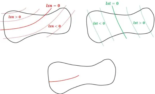
The arbitrary discontinuities are localized thanks to level set functions. An arbitrary interface is introduced thanks to a single level set function which represents the normal distance to the interface surface. The interface then corresponds to the iso-zero of this level set. In this article, this level set function is named the normal level set or 𝑙𝑠𝑛. When it comes to describing arbitrary cracks, two level sets are necessary. The first one still marks the normal distance to the crack surface, regardless of the presence of the crack front. The second one, the tangential level set (𝑙𝑠𝑡), is the tangent distance to the crack front with respect to the crack surface. The crack is defined as the set of points 𝒙 that satisfy: {𝑙𝑠𝑛(𝒙) = 0_{𝑙𝑠𝑡(𝒙) < 0. The level sets are often chosen as distance functions satisfying: {}‖𝛁𝑙𝑠𝑛‖ = 1_{‖𝛁𝑙𝑠𝑡‖ = 1} and given their definition, they must also satisfy: 𝛁𝑙𝑠𝑛 ∙ 𝛁𝑙𝑠𝑡 = 0

On Figure 2 (bottom), we observe the arbitrary crack described by a normal level set (top left) and a tangential level set (top right).

Figure 2: on the use of level set functions to describe arbitrary discontinuities.

In the implementation we have chosen and which is the most common, the level set functions are approximated by the same shape functions as the displacement field (see [Moës**]). This enables the crack shape to be described entirely in terms of nodal values. Of course this is not necessary nor always most convenient and one could chose to work with the functions themselves. However, in case of automatic propagation, the functions are not known explicitly and their numerical estimates at the nodes provide the only information to characterize them. So from now on, we abusively use the expressions “normal level set” and “tangential level set” to designate the discretized level sets. The crack Г depicted by the original level set functions is then discretized within the finite element mesh by means of the discretized level set functions. The resulting discretized discontinuity is denoted Гℎ. Finally, the elements crossed by Гℎ are split into integration subcells approximating the

discontinuity (quadratic integration subcells in the quadratic case and linear ones in the linear case). The resulting approximation of the crack is denoted Г̃and does not necessarily coincide with the

discretized crack Гℎ [Ferté1**] (see Figure 4). In order to measure the error introduced in this two

steps process, we compute the resolution 𝜀 defined as follow: 𝜀 = 𝑚𝑎𝑥_𝒙∈𝛤(𝑚𝑖𝑛_{𝒙̃∈Г̃}|𝒙 − 𝒙̃|)

For each point 𝒙 of the theoretical interface 𝛤, we compute the distance to the approximated interface 𝑚𝑖𝑛𝒙′∈Г̃|𝒙 − 𝒙̃|. Finally, we take the maximum over 𝒙 ∈ 𝛤. The resolution 𝜀 is then the

maximal distance between the analytical interface and the approximated inteface. Ferté ([Ferté1**]) showed that the resolution is proportional to ℎ2 in the linear case and ℎ3 in the quadratic case, ℎ denoting the representative size of the elements of the mesh, provided that the theoretical crack 𝛤 has sufficient geometric continuity.

Figure 4: the analytical arbitrary interface 𝜞 (left), the discretized iso-zero of the normal level set 𝛤ℎ (middle) and the approximated interface 𝛾 (right).

1.3 Domain integration

The approximation of the displacement field is discontinuous across the crack (equation (2)) so that the quantities we have to integrate over the domain 𝛺 (equation(1)) are also discontinuous. In order to integrate discontinuous quantities on each side of an interface, a first step consists in the design of a physical support for each sub-domain so that we can use the classical integration techniques on each continuous domain. We aim at getting a quadratic accurate approximation of the sub-domains cut off by the arbitrary discontinuities.

In order to obtain an approximation of the sub-domains, we identify the elements of the mesh that are crossed by an arbitrary discontinuity and divide them into integration subcells in compliance with the discontinuity. Within an element that includes a crack front, we perform this cutting procedure regardless of the presence of the crack front (Figure 3). The presence of the crack front is then eventually taken into account with specific degrees of freedom associated to singular enrichment functions [Dolbow**] [Béchet**] or with internal variables within the framework of cohesive zone model [Ferté2**]. In the approach proposed by Minnebo et al. [Minnebo**], the elements of the mesh that include the crack front are cut with respect to the crack surface only: {𝑙𝑠𝑛 = 0} ∩ {𝑙𝑠𝑡 < 0}, so that the crack front position is topologically induced by the set of integration subcells. But the extension of this method to 3D models is laborious. Two types of elements are then concerned by the cutting procedure for a crack:

- The elements that are entirely crossed by a discontinuity. The edges of these elements are strictly intersected by the iso-zero of the normal level set and on each of these intersection we satisfy 𝑙𝑠𝑡 < 0.

- The elements that are cut by the discontinuity and include a piece of the crack front. The edges of these elements are strictly intersected by the iso-zero of the normal level set and on the set of intersection points we satisfy max{𝑙𝑠𝑡} ∗ min {𝑙𝑠𝑡} < 0.

Figure 3: a crack on a regular mesh (left) and the triangular integration subcells generated in the elements crossed by the crack (right).

Once the cutting procedure is done, we can make the distinction between two meshes. The initial mesh whose nodes carry the degrees of freedom of the problem and the mesh resulting from the elements of the initial mesh that are not cut and the integration subcells designed to fit the arbitrary discontinuities. We denote this second mesh integration mesh, it is used for the domain integration but also for post-processing with visualization tools.

The difficulty of the problem lies in the construction of the integration subcells. We must have a systematic and robust procedure that manages to shape quadratic sub-elements fitting arbitrary discontinuities for 3D models with curved cracks. To our knowledge, there are few methods described in the literature [Fries**] for the cutting of 3D elements in the quadratic case. In the following, we propose a robust method to consistently create quadratic subcells fitting a crack surface in the 3D case.

Part 2: Partitioning 3D domains with arbitrary discontinuities

2.1 Overview of the cutting procedure

Our cutting procedure performs without refinement. We may then fail to identify small inclusions embedded within a single element, but we assume the user is aware of the relative size of the element of the mesh compared to the refinement of the level sets. On the contrary, the approach proposed by Fries et al [Fries**] uses a sample grid to detect eventual changes in the sign of the level set within the elements of the mesh. Adaptative remeshing with quadtree and octree meshes have also been studied in the extended finite method [Legrain**]. These methods enable a finer approximation of the immersed discontinuities and reduce the number of topologically distinct cutting configurations. Similarly to the approach of [Fries**], we build integration subcells fitting the arbitrary discontinuities with a quadratic accuracy. Then, we recover a reconstructed approximation of the immersed interfaces as the set of faces of the integration subcells coinciding with the discontinuities. Two noticeable features of our cutting procedure are the systematic preliminary reduction into primary elements and the level set adjustment procedure. This considerably reduces the number of topologically distinct cutting configurations we may encounter. The determination of the intersection points between the mesh and the immersed boundaries is systematically performed in the reference configuration of the elements so that the overall cutting procedure only relies on a one dimensional root-finding algorithm. We expect a quadratic convergence for this Newton-Raphson algorithm. Since the procedure depicted in this paper has been implemented in industrially

oriented finite element software, all the annoying cases have been identified and thoroughly treated. An overview of the overall cutting procedure, including the design of the integration subcells and the recovery of the contact faces, is summarized in Annex 1. Finally, the integration procedure detailed in sections 2 and 3 is entirely applicable for linear models. The difference lies in the fact that middle nodes are not necessary in the linear case for the voluminous integration subcells as well as for the contact faces.

2.2 Level set adjustments

In the linear case, the intersections between the iso-zero of the discretized normal level set with the mesh are found two ways:

- If at a node of the mesh 𝑙𝑠𝑛(𝑁) = 0, then the node is located on the iso-zero,

- If at the edge linking node A and B 𝑙𝑠𝑛(𝑁𝐴) ∗ 𝑙𝑠𝑛(𝑁𝐵) < 0, then the position of the

intersection point 𝐼 is given by: 𝐼 = 𝑁𝐴+_{𝑙𝑠𝑛(𝑁}𝑙𝑠𝑛(𝑁𝐴)

𝐴)−𝑙𝑠𝑛(𝑁𝐵)𝑁⃗⃗⃗⃗⃗⃗⃗⃗⃗⃗⃗ (see Figure 5), if the level set 𝐴𝑁𝐵 is a distance function.

The quadratic case requires more attention. The intersections between the iso-zero of the discretized normal level set and the mesh are localized:

- At the nodes of the mesh satisfying 𝑙𝑠𝑛(𝑁) = 0

- On any edge strictly cut by the the iso-zero of the discretized normal level set.

But the condition for an edge to be cut is not similar to the linear case. Indeed, along the edge of a quadratic mesh, the discretized level sets are marked at three locations: the two end nodes and the middle node. This leads to potential double cancelation of the discretized level sets along an edge (see Figure 5).

Figure 5: an intersection between the iso-zero of the normal level set and an edge in the linear case (left) and a case of double cancelation of the normal level set along an edge in the quadratic case

(right).

In the end, the condition for an edge to be strictly cut by the iso-zero of the normal level set in the quadratic case is: max{𝑙𝑠𝑛(𝑁𝐴), 𝑙𝑠𝑛(𝑁𝐵), 𝑙𝑠𝑛(𝑁𝑀)} ∗ min {𝑙𝑠𝑛(𝑁𝐴), 𝑙𝑠𝑛(𝑁𝐵), 𝑙𝑠𝑛(𝑁𝑀)} < 0. The

choice is made to restrict the situations of double cancelation of the normal level set along an edge in order to reduce the number and the complexity of the cutting configurations. For this aim, we proceed to level set adjustments.

The only cases of multiple cancelations of the discretized normal level set along an edge we accept are depicted in Figure 6:

Figure 6: the two cases of multiple cancelations of the level sets along a three node edge which are authorized.

Either the normal level set is null for each node of the edge, either it is null for one vertex node and the middle node. We also forbid the case where the iso-zero of the normal level set brushes against

an edge: {𝑙𝑠𝑛(𝑁_{𝑙𝑠𝑛(𝑁}𝐴) ∗ 𝑙𝑠𝑛(𝑁𝐵) > 0

𝑀) = 0 . Four situations encountered with the discretized normal level set

must then be adjusted. They are depicted on Figure 7.

Figure 7: level set adjustments along an edge.

For each case, we modify the value of the discretized normal level set at some nodes to be reduced to one of the two configurations of Figure 6.

Each time an adjustment is performed we introduce an error because we modify the value of the discretized normal level set at one or two nodes. The approximated iso-zero of the normal level set 𝛤ℎis then shifted (see Figure 4). It is not an optimal solution. As soon as we make adjustments, the

convergence properties for the approximation of the sub-domains may not apply. But this choice is justified by the following arguments:

- the restriction of the double cancelation situations significantly reduces the number and the complexity of cutting configurations.

- the adjustments are likely to happen only when the iso-zero of the discretized level set is highly curved and close to an edge. The use of thinner meshes always ends up solving the problem.

- the code is able to return a message each time an adjustment is performed. And in order to provide an indication on the error introduced, we measure the shift realized relatively to the range of the level set values over the support of the shifted node.

Remarks:

 when an adjustment is performed on an edge, it can induce a situation that requires an adjustment on an adjacent edge. So the procedure is performed recursively until no more adjustment is needed.

 the exact same procedure is applied to the discretized tangential level set.

2.3 Reducing the problem

Before we begin the treatment of an element that needs to be cut, we perform a prior treatment in order to reduce the problem. In the reference configuration of the parent element, we systematically split the non-simplex elements into a set of simplex cells: tetrahedral elements for 3D models and triangles for 2D models. In this way, we only have one type of cell to consider for the cutting procedure. It considerably reduces the number of cutting configurations we may come across. In Figure 8 and 9, we depict the partitioning of the non-simplex elements into simplex cells.

Figure 8: Partition of a quadrangle into two triangles (left) and partition of a pyramid into two tetrahedral elements (right).

Figure 9: Partition of a pentahedron into three tetrahedral elements (left) and partition of a hexahedron into six tetrahedral elements (right).

We denote the set of simplex cells obtained as the primary simplex cells. For the simplex elements, the set of primary simplex cell is composed by the element itself.

In the quadratic case, this partitioning induces the apparition of internal edges and additional nodes. These additional nodes were not part of the initial mesh; they are fictitious nodes that do not carry degrees of freedom. As the internal edges were not part of the original mesh, they were not concerned by the level set adjustment procedure. We can thus observe double cancelations of the level sets along these internal edges. This would bring undesirable cutting configurations. A solution to bypass this problem is explained in Section 2.5. It relies on the fact that we can choose between different partitions for the non-simplex elements.

Indeed there is not a unique manner to split a quadrangular element into two triangles, there are two (see Figure 10). The same goes for the pyramidal elements. There are two eligible sets of tetrahedral elements depending on how the internal edge splits the quadrangular face. For the pentahedron, we count 6 different manners to obtain a partition of 6 tetrahedral elements (see Figure 10). Finally, there are 6 different ways to partition a hexahedron into two pentahedra (see Figure 10). So we expect a maximum of 63different manners to partition a hexahedron into 6

tetrahedral elements. But amongst these 63different possibilities, a lot are identical due to symmetries and we only keep those who ensure the conformity between the different tetrahedral elements. One can show we are left with 72 distinct manners to partition a hexahedron into 6 conforming tetrahedral elements. These different manners to partition the non-simplex elements into primary simplex cells constitute splitting configurations. We keep in store the possibility to select these different configurations. As we will observe in Section 2.5, the use of these different configurations is essential to prevent the apparition of undesirable double cancelation of the level set along the edges of the primary simplex cells.

Figure 10 : the two different configurations for a quadrangular element (left), the 6 different configurations for a pentahedron (middle) an the six different ways to partition an hexahedron into

two pentahedra (right).

All the elements of the mesh that need to be cut are now split into a partition of simplex cells. The problem is now reduced to the cutting of simplex cells with respect to the iso-zero of the normal level set.

2.4 Intersections between the primary simplex cells and the iso-zero of the tangential level set For all the elements that need to be cut, we loop over the primary simplex cells and determine the intersections with the iso-zero of the discretized normal level set. For each primary simplex cell:

- we loop over the vertex nodes and identify those who coincide with the iso-zero of the normal level set (𝑙𝑠𝑛(𝑁) = 0). We denote as 𝑛𝑠 the number of intersection points coinciding

with vertex nodes of the primary simplex cell.

- we loop over the edges and for those verifying 𝑙𝑠𝑛(𝑁𝐴) ∗ 𝑙𝑠𝑛(𝑁𝐵) < 0, we determine the

position of the intersection point. If 𝑙𝑠𝑛(𝑁𝑀) = 0, the intersection point directly coincides

with the middle node 𝑁𝑀. In the opposite case, we use the root finding algorithm 1 to

determine the position of the intersection point. We denote by 𝑛𝑒 the number of edges

intersected by the iso-zero of the normal level set which includes the edges intersected at one vertex node and at the middle node (see Figure 6)

Remark: the unwanted cases of double cancelation of the iso-zero of the normal level set along an edge are ignored at this stage. They will be detected and cured during the next step (Section 2.5)

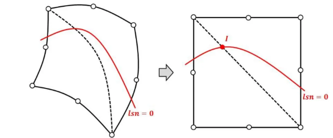
In order to determine the position of an intersection point on the edge of a primary simplex cell, we move to the reference configuration of the parent element and use a Newton-Raphson algorithm. The relocation in the reference configuration of the parent element presents two major advantages:

- the edges of the primary simplex cells are necessarily straight in the reference configuration of the parent element (see Figure 11).

- the convergence criterion for the Newton-Raphson algorithm is the same for all edges.

Figure 11: a quadrangular element crossed by the iso-zero of the normal level set in the real space (left) and in the reference configuration (right).

A parameterization of a straight edge 𝑁𝐴𝑁𝐵in the reference space is: = 𝑁𝐴+ 𝑡 ∗ 𝑵⃗⃗⃗⃗⃗⃗⃗⃗⃗⃗⃗⃗ , 𝑡 ∈ [0, 1] 𝑨𝑵𝑩

Algorithm 1 determines the intersection point between the iso-zero of a discretized level set and a straight line within an element. It only requires an initial guess of the position of the zero-level set and a unit vector carrying the search direction.

𝒖

⃗⃗ = 𝑵⃗⃗⃗⃗⃗⃗⃗⃗⃗⃗⃗⃗⃗ 𝑨𝑵𝑩

‖𝑵⃗⃗⃗⃗⃗⃗⃗⃗⃗⃗⃗⃗⃗ ‖𝑨𝑵𝑩 provides the unit vector and a relevant initial guess is the linear approximation: 𝐼0= 𝑁𝐴+_{𝑙𝑠𝑛(𝑁}𝑙𝑠𝑛(𝑁𝐴)

𝐴)−𝑙𝑠𝑛(𝑁𝐵)𝑵⃗⃗⃗⃗⃗⃗⃗⃗⃗⃗⃗⃗ 𝑨𝑵𝑩

Algorithm 1: Research of an intersection point between the iso-zero of a level set and a straight line within an element

 We set 𝑛 to 0, 𝛼0 to 0 and ∆𝛼0 to 2𝜀

 While |∆𝛼𝑛| > 𝜀

o 𝑛 = 𝑛 + 1

o 𝐼_𝑛= 𝐼_𝑛−1+ ∆𝛼_𝑛−1𝒖⃗⃗

o Compute the shape functions 𝜑𝑖 associated to the nodes of the parent element for

𝐼_𝑛

o Interpolate the value of the level set 𝑙𝑠(𝐼𝑛) = ∑𝑛𝑜𝑑𝑒𝑠𝜑𝑖𝑙𝑠𝑖

o Compute the derivative of the level set field along the unit vector 𝒖⃗⃗ : 𝛁⃗⃗ 𝑙𝑠(𝐼𝑛). 𝒖⃗⃗

o ∆𝛼_𝑛= − 𝑙𝑠(𝐼𝑛)

𝛁 ⃗⃗ 𝑙𝑠(𝐼𝑛).𝒖⃗⃗

 Return 𝐼𝑛

Tolerance 𝜀 is about a displacement increment in the reference configuration of the parent element. It is common to all elements and edges. Since the level set field are polynomial within an element, we expect a quadratic convergence for the Newton-Raphson algorithm.

Remark: when we look for an intersection point on an edge that coincide with an edge of the parent element, the discretized level set field only depends on the values of the level set at the three nodes of the edge. We could directly get the position of the intersection point from the resolution of a second order polynomial equation.

2.5 Shaping the integration subcells

Once we have determined the intersections between the primary simplex cells and the iso-zero of the normal level set, we associate to each primary simplex cell a cutting configuration. There is a total of 3 cutting configurations in the 2D case and 9 cutting configurations in the 3D case. The different cutting configurations are distinguished with the number 𝑛𝑠 of intersection points

coinciding with vertices nodes and the number 𝑛𝑒 of edges intersected by the iso-zero of the normal

level set.

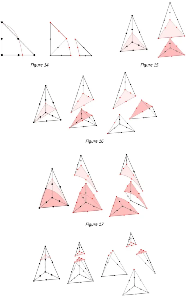
In the following, we detail the different cutting configurations encountered in 2D and 3D. The table hereunder gives the number of subcells generated by the primary simplex cells for each cutting configuration. On Figure 12 to 23, we depict the different cutting configurations, the iso-zero of the tangential level set appearing in red. The nodes and the edges of the primary simplex cells that coincide with this iso-zero also appear in red.

𝒏_𝒆 𝒏_𝒔 Number of subcells generated Figure

2D 1 1 2 12 2 0 3 13 2 1 3 14 3D 1 2 2 15 2 1 3 16 2 2 3 17 3 0 4 18 3 1 4 19 3 2 4 20 4 0 6 21 4 1 6 22 3 1 5 23

Table 1: cutting configurations for the primary simplex cells.

Remark: there are two configurations labeled {𝑛_𝑛𝑒= 3

𝑠= 1. The first is distinguishable from the second one because it has a common vertex for all three intersected edges.

Figure 14 Figure 15

Figure 16

Figure 17

Figure 19

Figure 20

Figure 22

Figure 23

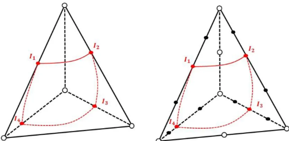
In order to maintain a quadratic accuracy in the approximation of the sub-domains on both sides of the discontinuity, the middle nodes of the integration subcells must be thoroughly determined. At this stage, we have only resolved the intersections between the primary simplex cell and the iso-zero of the normal level set so that we have at our disposal the entire set of vertex nodes for the integration subcells. In the following, we detail the determination of the middle nodes for the 3D configuration {𝑛_𝑛𝑒= 4

𝑠 = 0. The procedure is similar for the other configurations. We distinguish 4 types

of middle nodes. Here again, the determination of these nodes is performed in the reference configuration of the parent element.

1st type of middle nodes

The edges of the primary simplex cell that are intersected by the iso-zero of the normal level set are split into two edges, one on either side of the discontinuity. We place the middle nodes on each of these edges. For an edge 𝑁𝐴𝑁𝐵 of a primary simplex cells intersected at point 𝐼, the positions of the

middle nodes are obviously 𝑁𝐴+1₂∗ 𝑵⃗⃗⃗⃗⃗⃗⃗ and 𝑁𝑨𝑰 𝐵+1₂∗ 𝑵⃗⃗⃗⃗⃗⃗⃗⃗ . On Figure 24, we observe the first type 𝑩𝑰

Figure 24: the primary tetrahedron with the 4 intersection points 𝐼1,2,3,4 (left) and the first type middle nodes (black circles) on its intersected edges (right).

2nd type of middle nodes

The second type middle nodes are located on the faces of the primary tetrahedron, between the intersection points, on the approximated discontinuity. For each intersected face, we search this middle node on the perpendicular bisector to the segment formed by the two intersection points. For example in Figure 26 (left), we search the middle node between 𝐼3 and 𝐼4 on the perpendicular

bisector to the segment [𝐼3𝐼4] on the bottom face of the primary tetrahedron. We still use algorithm

1 to locate these middle nodes. But we must ensure that the middle node stays confined in the face of the current primary simplex cell. Indeed, for non-simplex elements, the middle node can be found in the adjacent primary simplex cell, giving away a situation of double cancelation of the tangential level set along an edge (see Figure 25). In order to detect this situation, we compute first the limits 𝑡_𝑖𝑛𝑓 and 𝑡𝑠𝑢𝑝 of the authorized interval along the perpendicular bisector. The middle of the segment

[𝐼3𝐼4] is then chosen as an initial guess and the vector 𝒖⃗⃗ is chosen as the unit vector on the

perpendicular bisector oriented along the gradient of the normal level set. Once the algorithm has converged, if the middle node is found out of the interval [𝑡𝑖𝑛𝑓, 𝑡𝑠𝑢𝑝], we go back to the splitting into

primary simplex cells (Section 2.3) for the parent element and select another configuration. For instance in Figure 25, we depict a 2D example of double cancelation of the normal level set along the internal edge of a quadrangle. The other splitting configuration succeeds in bypassing the problem. The 3D cases are similar. There might be some extreme cases for which no conformation succeeds in bypassing the problem. In that case, we perform a local linear approximation of the discretized normal level set. But these insolvable cases would definitely present very twisted level sets and a mesh refinement would surely solve the problem.

Figure 25: a case of double cancelation of the normal level set along the internal edge of a quadrangle. The middle node 𝑀 between 𝐼1and 𝐼2 is found out of bounds (left). The other configuration is selected to split the quadrangle into two primary triangles, bypassing the problem

Figure 26: determination of the middle node between 𝐼3 and 𝐼4 (left) and the primary tetrahedron with the second type middle nodes 𝑀1,2,3,4 (right).

3rd type of middle nodes

The third type middle nodes are located on the triangular faces of the primary simplex cells intersected by the discontinuity. These faces are split into a triangle and a quadrangle (see Figure 27 left). The quadrangle 𝑁1𝑁2𝐼2𝐼1 is supposed to be split into two triangles. For this aim, we determine

the middle node between 𝐼2 and the opposite vertex node 𝑁1. Whenever possible, we choose the

middle of the segment [𝐼2𝑁1] as the middle node 𝐶 which generates one twisted sub-triangles

instead of two (see Figure 27). But this choice may not be convenient when the discontinuity is highly curved. On Figure 27, the case depicted at the bottom left generates distorted sub-triangles if the middle node 𝐶 is chosen as the middle of the segment [𝐼2𝑁1]. In that case, we choose the middle of

the quadratic quadrangle for 𝐶. In order to detect these situations, we compute the tangent vector 𝑗 to the three node segment 𝐼2𝑀𝐼2 at the point 𝐼2 (see Figure 27). Depending on its position compared

to the tangent vector 𝑘⃗ to the segment 𝐼2𝑁1, we choose a different type of construction for the

localization of the middle node 𝐶.

Figure 27: determination of the third type middle node: 𝐶 is chosen as the middle of the segment

[𝐼₂𝑁₁] (top left) and 𝐶 is chosen as the center of quadrangle 𝑁1𝑁2𝐼2𝐼1 (bottom left). The primary tetrahedron with the third type middle nodes in green (right).

4th type of middle nodes

The last type of middle nodes are the ones located in the middle of the quadrangular faces approximating the iso-zero of the tangential level set. On Figure 28, we look for the middle of quadrangle 𝐼1𝐼2𝐼3𝐼4. The middle of segment [𝐼2𝐼4] is chosen as an initial guess and for the unit vector

𝒖

⃗⃗ carrying the straight search path, we choose the normalized gradient of the normal level set. Indeed, the gradient of the tangential level set gives the normal direction to the interface, it forms the best search direction. Once again, first we determine the authorized interval [𝑡𝑖𝑛𝑓, 𝑡𝑠𝑢𝑝],

corresponding to the intersection between the search direction and the primary tetrahedron. If the middle node is found out of bounds, we go back to the splitting into primary simplex cells and select another configuration.

Figure 28: determination of the fourth type middle node in the interval [𝑡𝑖𝑛𝑓, 𝑡𝑠𝑢𝑝] (left) and the primary tetrahedron with the four types of middle nodes (right).

Now that all the nodes of the integration subcells have been determined, the primary simplex cells are split into integration subcells according to the cutting configurations depicted in Section 2.5. The integration subcells are labeled with the sign of the normal level set, depending on which side of the discontinuity they belong to. The nodes of the integration subcells coinciding with the iso-zero of the normal level set are also specifically labeled.

2.6 An extension to multi-cracked models

The splitting into integration subcells can be extended to multi-cracked models, in particular to branching discontinuities. For the elements crossed by several discontinuities, the procedure depicted for one interface is performed iteratively.

To each arbitrary discontinuity is associated a normal level set field. For branching discontinuities, the branched discontinuities are defined only on one side of a main discontinuity. On Figure 29, the second discontinuity (in green) is branched on the first discontinuity (in red) and defined only in the domain {𝑙𝑠𝑛1> 0}. The third one (in blue) is branched on the second one, which was branched on

Figure 29: definition of branched arbitrary discontinuities by means of normal level set.

For an element crossed by several discontinuities, we proceed one discontinuity after another. For the first discontinuity, the procedure depicted above is normally performed. We end up with a set of integration subcells fitting the first discontinuity. For the cutting with respect to the second discontinuity, we proceed in the same way as for the first discontinuity except that the set of primary simplex cells is replaced by the set of integration subcells we obtained during the first cutting procedure. The difference lies in the fact that the edges of the integration subcells are not necessarily straight in the reference configuration of the parent element, contrarily to the edges of the primary simplex cells. In order to bypass this problem and apply the exact same procedure as for a single discontinuity, we work on the reference configuration of the integration subcells to perform the cutting procedure with respect to the second discontinuity. In this way, we always end up cutting simplex cells with straight edges. The procedure is summarized in Figure 30. The quadrangle is crossed by a main discontinuity (in red) and a branched discontinuity (in green). We work in the reference configuration of this quadrangle to perform the cutting with respect to the first discontinuity. Then we loop over the resulting integration sub-triangles. For each of them, we work in the reference configuration of the sub-triangle and apply the procedure depicted in Sections 2.3 to 2.5.

On Figure 31, we observe the final integration sub-triangles obtained for the quadrangle, fitting both discontinuities. The nodes coinciding with the first discontinuity appear in red and the nodes coinciding with the second discontinuity appear in green. The junction point is green and circled in red.

Figure 31: final integration sub-triangles for the quadrangle.

Similarly to the single discontinuity case, the integration subcells are labeled with the signs of the normal level sets, depending on which side of the discontinuities they belong to. When the level set is not defined (in the case of branching discontinuities), the default sign is 0. The nodes of the integration subcells coinciding with the iso-zero of the tangential level sets are also specifically labeled. In particular, the junction points are labeled for both discontinuities.

2.7 Integration over the sub-domains

Now that we split the elements crossed by arbitrary discontinuities into sets of integration sub-cells, making up an accurate quadratic approximation of the sub-domains, we are in position to realize a domain integration. Indeed, the integration subcells were labeled depending on which sub-domain they belong to. We can thus recover exclusively the set of elements and subcells approximating any sub-domain. For the volume integration over the integration subcells, we use the Standard Gauss integration techniques. The Gauss integration schemes we use are summarized hereunder. According to [Dathe**], the use of order 3 Gauss integration schemes in the linear case and order 5 Gauss integration schemes in the quadratic case offers satisfactory accuracy for the integration of the left side terms of equation (1) over tetrahedral elements.

Subcell Number of Gauss integration points per subcell

order

2D Linear case 3 node triangle 3 3

Quadratic case 6 node triangle 6 5

3D Linear case 4 node tetrahedron 5 3

Quadratic case 10 node tetrahedron 16 5

Part 3: integration on the crack surface

Now that we have designed the volumetric integration subcells in the elements crossed by arbitrary discontinuities, we have to obtain a reconstructed iso-zero of the normal level set to achieve integration on the crack. Indeed, the integration on the crack surface is useful for various applications of the extended finite element method. For instance, the contact efforts preventing the interpenetration between adjacent subdomains are usually integrated on the crack surface [Géniaut**][Pierrès**] as well as the cohesive efforts when the propagation of the crack is governed by a cohesive zone model [Ferté2**]. The consideration of a fluid pressure on the fracture walls in the case hydraulic fractures [Faivre**] also requires a material approximation of the zero-level set . The volumetric subcells were built in order to offer a quadratic approximation of the domains separated by the arbitrary discontinuities. Thus the approximation of the different domains includes an approximation of the discontinuities. We use the faces of the subcells that coincide with the discontinuities to build the reconstructed implicit interfaces. When the element includes a piece of a crack front, a final cutting procedure with respect to the tangential level set is necessary to obtain a reconstructed approximation of the crack surface and front.

3.1 Overview of the recovery of the contact faces

The set of faces approximating an implicit interface is designed hereafter the contact faces as one of their main use is the integration of the contact equations between adjacent sub-domains. We impose an absolute fit between the integration subcells and the contact faces. The fit is clear for the contact faces that are directly recovered from the integration subcells. But when an element includes a piece of the crack front, the contact faces recovered from the integration subcells must be cut with respect to the normal level set associated to the crack front. In order to maintain the fit with the integration subcells and the quadratic accuracy throughout this final cutting procedure, we use the tools depicted in Part 1. In the end, the cutting procedure for the contact faces relies on the cutting procedure performed for the integration subcells.

3.2 Contact faces for an element entirely cut by an interface

First of all, we focus on the elements entirely crossed by a single arbitrary discontinuity. These elements have already been split up into tetrahedral integration subcells (triangular integration sub-cells in the 2D case). Some faces of theses subsub-cells correspond to the quadratic approximation of the arbitrary discontinuity. The vertex nodes of these faces were specially labeled when we shaped the integration subcells because they correspond to the intersections between the discontinuity and the edges of the primary simplex cells. As a consequence, we only need to loop over the faces of the integration subcells and select those whose 3 vertex nodes are labelled as intersection nodes (see Figures 32 and 33). In order to get each contact face exactly once, the choice is made to extract them only from the subcells labeled with a negative signed distance function.

Figure 32: extracting the contact faces from a quadrangular element: triangular integration subcells (left) and resulting contact faces (right).

Figure 33: extracting the contact faces from a hexahedral element: tetrahedral integration subcells (left) and resulting triangular contact faces (right).

3.3 Contact faces for an element which includes a piece of the crack front

For the elements that include a piece of the crack front, another complementary cutting procedure is necessary. Indeed, the design of the integration subcells detailed in part 1 was realized regardless of the crack front. All the elements that intersect the discontinuity were split with respect to the normal level set. But in order to perform an integration over the surface of discontinuity, it is necessary to have contact faces that match the crack front depicted by the iso-zero of the tangential level set.

The first step consists in extracting the preliminary contact faces in the same manner as in the previous section. Then, we compute the value of the tangential level set at the vertex nodes of these preliminary contact faces and classify them into 3 groups:

- the contact faces whose 3 vertex nodes satisfy 𝑙𝑠𝑡 ≥ 0 form the group 1. This group is out of bounds, its elements will be eliminated.

- the contact faces whose 3 vertex nodes satisfy 𝑙𝑠𝑡 ≤ 0 form the group 2. We keep this entire group for the final contact faces.

- the remaining contact faces that are necessarily intersected by the iso-zero of the tangential level set form the group 3. These contact faces need a further cutting out.

In the 2D case, the intersection between the iso-zero of the tangential level set and a preliminary contact face of group 3 is determined with algorithm 1 in the reference configuration of the contact face (so that the contact face is a straight segment). Then, the new middle node of the contact face

(type 1 middle node) is mapped from the reference configuration of the segment to the contact face in the parent element. The procedure is summed up in Figure 34.

Figure 34: extracting the contact faces from a quadrangle that includes the crack front. 1 - amongst the preliminary contact faces, we keep those whose vertex nodes satisfy 𝑙𝑠𝑡 ≤ 0 and select the ones intersected by the iso-zero of the tangential level set for the cutting procedure (top left),

2 - we determine the intersection between the contact face and the iso-zero of the tangential level set (top right), 3 - we determine the new position of the middle node of the intersected contact face (bottom right),

4 - we get the final contact faces(bottom left).

The 3D case requires more attention, amongst the triangular contact faces of group 3, we distinguish 3 cutting configurations:

- the contact faces that have one vertex node satisfying 𝑙𝑠𝑡 = 0 (configuration 1) - the contact faces that have two vertex nodes satisfying 𝑙𝑠𝑡 < 0 (configuration 2) - the contact faces that have one vertex node satisfying 𝑙𝑠𝑡 < 0 (configuration 3)

Figure 35: the 3 cutting configurations for the contact faces.

The criterion we use to determine whether a contact face is entirely in the domain {𝒙|𝑙𝑠𝑡(𝒙) ≤ 0} or entirely in the domain {𝒙|𝑙𝑠𝑡(𝒙) ≥ 0} or intersected by the iso-zero of the tangential level set only lies on the vertex nodes of the contact faces. We might then face situations for which the values of the tangential level set at the middle nodes of the contact faces contradict this classification, giving away a double cancelation of the tangential level set along the edge of the contact face. At first, we assume these situations do not occur. The last part of this section is dedicated to the treatment of these annoying cases.

In the following, we explain the cutting procedure for the second cutting configuration. The task consists in cutting a triangle with respect to the tangential level set. In the reference space of the parent element, this triangle is not necessarily plane as it approximates the iso-zero of the normal level set. In order to be reduced to the cutting procedure depicted in Sections 2.3 to 2.5, we use the same ingredient as in the case of multi-cracked elements. We map the preliminary contact face with its associated reference triangle whose edges are straight. Then, we apply the classic procedure for the cutting of 2D triangular element (Figure 36).

Figure 36: cutting a triangular primary contact face into two triangular final contact faces within a tetrahedral element.

On Figure 37, we observe the two final triangular contact faces in the primary tetrahedral element. They fit the iso-zero of the tangential level set.

Figure 37: final contact faces in the primary tetrahedral element.

The cutting procedure is similar for the two other configurations. As depicted in Figure 38, they both give one final triangular contact face.

Figure 38: the final contact faces for the 3 cutting configurations.

Finally, we look at the situations of double cancelation of the tangential level set along an edge of the preliminary contact faces. On Figure 39, we observe the preliminary contact faces generated by a planar crack in a hexahedron.

The tangential level set cannot cancel twice on the edges of the preliminary contact faces that coincide with a face of the parent element because we previously performed the level set adjustment (Section 2.2). But on the edges of the preliminary contact faces that are internal to non-simplex parent element, we cannot prevent a potential double cancelation of the tangential level set. Two distinct situations may occur. The first situation is depicted in Figure 40. It corresponds to a double cancelation of the tangential level set along the edge of a preliminary contact face due to a local high convexity of the crack front. This situation is detected when we look for the middle node 𝑀 between the two intersection points 𝐼1and 𝐼2. The middle node 𝑀 is found out of the bounds since it

exceeds the upper limit 𝑡𝑠𝑢𝑝. Contrarily to what was done in Part 1 for the integration subcells, we

authorize the middle node 𝑀 to go over the upper limit 𝑡𝑠𝑢𝑝. Indeed, the nearby preliminary contact

face affected by the intrusion stands in group 1 and will be eliminated. In this way, we obtain an accurate quadratic approximation of the crack surface.

Figure 40: situation 1.

The second situation is depicted in Figure 41. It corresponds to a double cancelation of the normal level set along the edge of a preliminary contact face due to a local high concavity of the crack front. This situation is detected when we look for the middle node 𝑀 between the two intersection points 𝐼1and 𝐼2. The middle node 𝑀 is found out of the bounds since it exceeds the lower limit 𝑡𝑖𝑛𝑓. In this

case, we cannot allow the intrusion of the middle node 𝑀 in the nearby preliminary contact face because it would bring distorted contact faces. One solution consists in making a local linear approximation of the tangential level set. The position of the middle node M is chosen as the initial guess of algorithm 1. In the reference space of the parent element, it is then the middle of the segment [𝐼1𝐼2].

This local linear approximation of the tangential level set seriously degrades the accuracy of our integration procedure. By all means, we would like to avoid it. The solution consists in going back to the very beginning of the cutting procedure for the parent element. We try the other eligible configurations for the partitioning of the parent element into primary simplex cells (Section 2.3) until no double cancelation of the level set is recorded. As depicted in Figure 42, these other configurations generate different primary simplex cells and different patterns for the preliminary contact faces, likely to bypass the problem depicted in Figure 41.

Figure 42: treatment of situation 2. 1 – first and previous configuration for the primary simplex cells (top left), 2 - another configuration of the primary simplex cells (top right),

3 - the new configuration of the primary simplex cells generates a new pattern of preliminary contact faces (bottom right),

4 - the new pattern of preliminary contact faces allows us to accurately approximate the crack surface in the vicinity of the crack front (bottom left).

As for the design of the integration subcells, we can imagine there might be some extreme cases for which no configuration succeeds in bypassing the problem of double cancelation of the level sets along an edge of a primary integration subcell and along an edge of a preliminary contact face. In that case, we perform local linear approximations of the discretized level set. But these insolvable cases would definitely present very twisted level sets. A mesh refinement would surely solve the problem.

Please note that these contact faces also allow us to obtain an accurate quadratic reconstruction of the crack front as a chain of 3 node segments for 3D models. It may be useful for fracture mechanics post-processing.

3.4 Contact faces for multi-cracked elements

In this section, we detail the recovery of the contact faces for multi-cracked elements. We only consider multi-cracked elements that do not include crack fronts. In order to recover the contact

faces of multi-cracked elements that include crack fronts, we would have to combine the procedure depicted in this section with the procedure depicted in the previous section.

The multi-cracked elements have already been split up into tetrahedral integration subcells (triangular integration subcells in the 2D case). As for the single-cracked elements, some faces of these subcells correspond to the quadratic approximation of arbitrary discontinuities. The vertex nodes of these faces were specifically labeled distinctly for each discontinuity when we shaped the integration subcells. In particular, the junction points were labelled for the two discontinuities forming the junction. So for each discontinuity, we proceed exactly as for a single discontinuity. We loop over the faces of the integration subcells and select those whose 3 vertex nodes are labelled as intersection nodes for the current discontinuity. In the case of a single discontinuity, the choice was made to loop only over the integration subcells labeled with a negative signed distance function in order to recover the contact faces exactly once. For multi-cracked elements, it is necessary to modify this rule for the main discontinuities. The main discontinuities are defined as the discontinuities on which another discontinuity is branched. For these discontinuities, we decide to recover the contact faces from the integration subcells labeled whether with a negative or a positive sign distance function depending on the position of the branched interface. We chose the sign corresponding to the side where the interface is branched. Then we loop over the integration subcells labeled with the corresponding sign to recover the contact faces for the main discontinuity. On Figure 43, we observe a quadrangular element including a branching discontinuity and the resulting triangular integration subcells fitting both discontinuities. The main discontinuity and the branched discontinuity delimit three distinct domains 𝛺1, 𝛺2 and 𝛺3 over the quadrangular element. On Figure 44, we observe the

resulting contact faces when we extract the contact faces for the main discontuity from the integration subcells labeled with a sign that does not correspond to the branching (left) and that does correspond to the branching discontinuity (right). In the first case, we end up with two contact faces for the main interface as if the branching was not existing. Then the contact face whose end nodes are 𝐼2 and 𝐼3 does not fit the junction as it was extracted from an integration subcell which is

not on the side of the branching discontinuity. In the second case, we end up with 3 contact faces for the main interface. They fit the discontinuity junction because they where extracted from integration subcells located on the side of the branched discontinuity. It is essential to obtain contact faces that fit both discontuities. For instance, we may want to perform a surface integration exclusively on the boundary separating 𝛺1 from 𝛺3. This is feasible provided that the contact faces for the main

discontinuity fit the branched discontinuity.

Figure 43: a quadrangular element including a branching discontinuity (left) and the resulting integration subcells (right).

Figure 44 : the resulting contact faces when we extract the contact faces of the main interface from the integration subcells located above (left) and below (right) the main interface.

When several discontinuities are branched on the same main discontinuity within an element, we may not be able to properly recover contact faces fitting all the junctions. On Figure 45 (left), we observe a quadrangular element crossed by a main interface (red) with two branched discontinuities. The discontuities are branched on both sides of the main interface. We also observe the resulting integration subcells. Neither the integration subcells located below the main interface neither the ones located above generate contact faces fitting both junctions for the main interface. This configuration can not be solved so that we forbid the presence of two distinct fracture junctions within the same element. This can easily be avoided by refining the mesh. However, we can still have branched fractures within the same element if the different junctions coincide (Figure 45 right).

Figure 45: a quadrangular element including two discontinuity junctions and the resulting integration subcells in the case of not coinciding junctions (left) and coinciding junctions (right).

3.5 Integration over the contact faces

Now that we have built contact faces that accurately approximate the immersed boundaries, we are in position to perform surface integrations over the sub-domain boundaries. For this aim, we use classical Gauss integration techniques. For each contact face, the positions of the Gauss integration points are interpolated from the position of the nodes of the contact face. Furthermore, the surface integration often requires the normal direction to the contact face (for instance to take into account a fluid pressure in the fracture). So for each Gauss point we build a unit normal vector to the contact

face (oriented along the gradient of the normal level set) from the position of the nodes of the contact face (see Figure 46).

Figure 46: integration over the curved contact faces of a quadrangle (left) and a hexahedron (right).

The Gauss integration schemes used for the surface integration are summarized hereunder. According to [Dathe**], the use of order 3 Gauss integration schemes in the linear case and order 5 Gauss integration schemes in the quadratic case offers satisfactory accuracy for the integration of the right side terms of equation (1) over triangular elements.

Contact face type Number of Gauss integration points per contact face

order

2D Linear case 2 node segment 2 3

Quadratic case 3 node segment 3 5

3D Linear case 3 node triangle 3 3

Quadratic case 6 node triangle 6 5

Table 3: Gauss integration schemes for the contact faces.

Part 4: validation of the integration method

In the following discussion, we present some numerical results in order to illustrate and validate the accuracy and robustness of the integration method detailed in the first two sections. In particular, we perform several convergence analyses. The convergence rates we get are in accordance with the theory. First of all, we present the XFEM formulation we combined to our integration procedure to perform the numerical tests.

4.1 Description of the XFEM formulation used

In the literature there are many formulations to model strong discontinuities in continuous media. In the paper of Ndeffo et al. [Ndeffo**], a thorough analysis has been made and numerical issues have been investigated, at least concerning quadratic elements. It has been established that partition

of unity based formulations don’t behave well in asymptotic configurations (when the discontinuity gets close to the nodes of the approximation mesh). Therefore, conditioning and accuracy issues need a special care when modeling higher order strong discontinuities. Hence, Ndeffo et al. suggests a convenient formulation to deal with the condition number swift increase. In this section, we extend the suggested formulation to the case of branching discontinuities. Before describing more precisely the aforementioned formulation, let’s focus on the definition of branching discontinuities. In the literature, there are two methods to define branched cracks:

 The use of sign fields called likewise “junction” functions: there are encountered in the framework of X-FEM and level-sets [Daux**].

 The use of non-overlapping domains in the “neighborhood” of the branched discontinuity: there are encountered in the framework of GFEM [Reno**].

The X-FEM defines iteratively the “junction” functions based on level-sets, to represent the branched crack kinematics. GFEM fits for the description of branching discontinuity when the information about domains is available; typically, in the case of polycrystals modeling, where partitions of the whole domain are well labeled [Poly**]. As we use level-sets to model discontinuity in this paper, an X-FEM description is more convenient.

However, the X-FEM enrichment functions perform poorly in terms of conditioning and accuracy for higher order elements, as shown in [Ndeffo**]. Formulations based on the partition in domains [Hansbo**],[Reno**], have a better numerical behavior. Thus our enrichment strategy should combine both features: the X-FEM its convenience and the formulations based on domains partitioning to deal with conditioning issues. As explained in [Ndeffo**], these two approaches are intermingled. Hence, we can switch from the description of branched discontinuities using level sets to the description using domain partitioning, more fitted for higher order elements. Before solving afore-mentioned conditioning issues, let’s stress again on the definition and assembling of X-FEM junction d.o.f.

Definition X-FEM/GFEM approximation spaces

In the case of multiple cracks, following the notations of equation (2), the GFEM/X-FEM approximation of the displacement field could be summarized as follows:

𝑢_ℎ(𝑥) = ∑ 𝜑_𝑖(𝑥)𝑢_𝑖

𝑖∈𝑁/𝑁𝑔

+ ∑ ∑ 𝜑_𝑗(𝑥)𝐻̃_𝑗,𝑘(𝑥)𝑎_𝑗,𝑘

𝑘=1,𝑐𝑎𝑟𝑑𝑗

𝑗∈𝑁𝑔

where 𝑁𝑔 represents the set of enriched nodes; 𝑁/𝑁𝑔 the set of non enriched nodes; 𝑐𝑎𝑟𝑑𝑗 the

node-wise number of d.o.f. for an enriched node, which depends of the number cracks intersecting the support of the node, and 𝑎𝑗,𝑘 the related d.o.f. 𝐻̃𝑗,𝑘 is a generic notation for whether X-FEM or

GFEM node-wise enrichment functions defined in the table below:

Single crack Single junction Double junction X-FEM {𝜑, 𝐻1𝜑} {𝜑, 𝐻1𝜑, 𝐻2𝜑} {𝜑, 𝐻1𝜑, 𝐻2𝜑, 𝐻3𝜑}

GFEM {𝜒𝛺1𝜑, 𝜒𝛺2𝜑} {𝜒𝛺1𝜑, 𝜒𝛺2𝜑, 𝜒𝛺3𝜑} {𝜒𝛺1𝜑, 𝜒𝛺2𝜑, 𝜒𝛺3𝜑, 𝜒𝛺4𝜑} NEW {𝜑, 𝜒𝛺2𝜑} {𝜑, 𝜒𝛺2𝜑, 𝜒𝛺3𝜑} {𝜑, 𝜒𝛺2𝜑, 𝜒𝛺3𝜑, 𝜒𝛺4𝜑}

Table 4 : comparison between node-wise enrichment functions in the case of X-FEM, GFEM and the NEW enrichment strategy proposed; where 𝐻𝑖 represents a sign-function and 𝜒𝛺𝑖 the characteristic